Smart Nutrient Deficiency Prediction System for Groundnut Leaf

1  Introduction

Groundnut is an important cash crop cultivated all over the world. The top three groundnut producing countries are China, India, and Sudan. The presence of chlorophyll is a crucial sign for determining the level of nitrogen in a crop, because the two variables are directly proportional. Timely monitoring of groundnut chlorophyll concentration (CC) can facilitate farmers’ knowing the field condition and providing an appropriate amount of fertilizer. Human observation will not be sufficient to identify the different categories of nutrient deficiency of crops before visible or tangible symptoms. Providing fertiliser after noticing severe symptoms may not work, which leads to an irrecoverable stage. Traditionally, the CC of any plant had been determined using a laboratory method, which was time-consuming [1]. In the case of finding more than one plant or leaf, it is costly, labor-intensive, and can only be measured in a destructive way. Hence, it is difficult to use in a real-time field during all growth periods of a crop. In recent decades, several portable devices have been developed and introduced by several researchers, such as the Soil Plant Analysis development (SPAD) Meter, which measures the relative chlorophyll content of plant leaves; atLEAF CHL PLUS, which measures the chlorophyll, Leaf Absorptance Meter measures white light reflectance and absorption on plant leaves. An oxygen metre measures the amount of oxygen present in plant soil samples. Quantum Sensor Meter-quantify the light intensity and A pyranometer measures a portion of the solar spectrum to measure the plant’s health or growth factors. These metres can measure the plant’s crop factors in a non-destructive way. However, it requires a high cost; therefore, smallholder farmers could not adopt these devices. In India, 82% of farmers are marginal or sub-marginal farmers. Apart from that, each portable metre has some demerits like coverage of a small area, not measurable with all sizes of leaves, and cannot be used in certain environmental conditions.

Satellite remote sensing is used to monitor large-scale crop fields and determine crop growth factors [2]. Nevertheless, weather conditions impact satellite-based remote sensing. Furthermore, it shows the resolution, time limitation, difficulty of serving in small fields, and cost of building. As an alternative option to remote sensing, Unmanned Aerial Vehicles (UAV) could be used to assess crop growth. One of the vital key parameters in UAV monitoring is the light source, which helps to estimate the growth factors of the crop [3]. Digital image analysis could be performed from the collected crop field images to determine the health condition of the crop. For image collection, the most commonly used cameras by researchers are hyperspectral, multispectral, and Red-Green-Blue (RGB). A hyperspectral camera with a high spectral band could furnish a rich source of information from crop fields [4]. But all the furnished information might not be necessary to identify the crop's health status, and determining the necessary information itself is a complex task. Further processing of the entire obtained information requires high resources and may lead to computational issues. As an alternative, a multispectral camera could be used for crop growth monitoring to extract features with a low number of spectral bands. But there is a high possibility of omitting the necessary information. Both cameras' main purpose is to extract the necessary features from the collected images, but they are too expensive for all types of farmers to use. While comparing both types of cameras with RGB cameras, the RGB camera is cheap and could be adopted by all types of farmers [5]. Rich source features can also be extracted from RGB images using advanced techniques like image processing, feature extraction, and convolutional neural networks. Therefore, it was feasible to use RGB images of groundnut crop leaves to determine the CC range. Smart Nutrient Deficiency Prediction System (SNDP) is proposed to detect and categorise the chlorophyll concentration range with the help of the RGB images and advanced techniques. So far, much research has been done to identify and classify the deficiency of crops with the help of advanced techniques. In most of the work, the data collection process is done using an RGB camera and a portable handheld device. A detailed explanation of those works is discussed in the literature survey section.

2  Literature Survey

Hydroponic experiments done by Xu et al., in rice crop [6], the total number of rice leaf images collected was 1818. From that, ten multi-nutrient deficiencies of the rice crop, such as nitrogen (N), potassium (P), phosphorus (K), calcium (Ca), magnesium (Mg), sulphur (S), manganese (Mn), iron (Fe), zinc (Zn), and silicon (Si), were diagnosed. Then the data was evaluated with four different deep convolution neural network (DCNN) state of the art techniques, including ResNet-50, Inception-v3, DenseNet-121, and NasNet-large, with a fine-tuning process. Among them, densenet121 performed best, with a validation accuracy of 98.62%. But they have not used outdoor images and the collected images are also not that extensive. Six categories of tomato leaf datasets were taken from the plant village website to assess the crop's health with four deep learning-based algorithms, including Resnet-50, VGG-19, Xeception, and Inception-v3. Among them, five are diseased classes and one is a healthy class. The factors considered for evaluating model performance by Prakruti et al., are inference time, memory utility, accuracy, and model size. In terms of accuracy, ResNet-50 obtained the highest training accuracy of 99.7%. But the same model was tested with a different dataset, which was collected under uncontrolled conditions and achieved an accuracy of 65.12%. This implies the importance of the data collection environment. In terms of memory utility, model size, and inference time, their results showed that VGG-19 was high as it extracted the maximum number of features [7]. Twelve different colour features were extracted from immature tea leaf images and they had been correlated with the chlorophyll level of those leaves, which had been measured using a SPAD meter. The extracted colour feature given as input to three different models is K Nearest Neighbour (KNN), MLR (Multi Logistic Regression), and 1-D CNN. The 1-D CNN model achieved the highest R-squared value of 81% and had a lower error rate compared to other machine learning models. The author has performed a comparative analysis with some existing leaf chlorophyll prediction models [8]. From that analysis, it can be observed that the compared models' performances are high in terms of accuracy, except for Yadav et al., model [9]. The ResNet-50 deep learning algorithm was used to detect red grapevine's potassium deficiency and achieved a test accuracy of 80%. The used dataset contains six varieties of 50 red grapevine leaf images. The performance of the model was compared with the Support Vector Machine (SVM) algorithm for which the leaf features were extracted with the Histogram of Oriented Gradients (HOG) descriptor and the obtained accuracy was 66.67% [10]. The authors have used limited leaf images. As a suggestion, increasing the number of images through the image preprocessing technique could provide even better performance with a model like ResNet-50.

A combination of old and young blackgram plants' datasets was used to find out the six different types of nutrient deficiency, such as Ca, Fe, P, K, Mg, N, and complete nutrients. The pre-trained ResNet-50 model was applied to the dataset to extract the features, and those features were given to three different machine learning models: Multi-Layer Perceptron (MLP), Logistic Regression (LR), and SVM. Among them, MLP model performance was superior, with an accuracy of 88.33% [11]. Eleven different vegetation indexes (VIS) were extracted from the rice images, which had been collected using a UAV during all growth periods. Then the nitrogen nutrient index (NNI) was calculated with the help of critical N concentration and above-ground biomass from rice fields. Zhengchao Qiu et al. discovered the strongest correlation between NNI and UAV-VIS during a specific growth period. Thus, the NNI of rice plants is predicted in various growth periods using VIs with the help of distinct machine learning algorithms including artificial neural network (ANN), partial least squares (PLSR), random forest (RF), KNN, SVM, and adaptive boosting (AB). Among them, RF obtained optimal coefficient of determination (R2) and Root Mean Square Error (RMSE) values ranging from 0.88–0.97 and 0.03–0.07, respectively. They also predicted the high correlation between NNI and yield in certain growth stages. Further, a stable correlation was found between soil available nitrogen and NNI [12].

A model was developed to estimate the chlorophyll measurement of the soya bean crop using machine learning and image processing techniques. The experimental analysis was performed with various vegetation colour indices and found that the Dark Green Colour Index (DGCI) had a high correlation with the chlorophyll handheld metre SPAD. The correlation range was further improved by the colour calibration method. Various colour scheme inputs are tested with simpler statistical models which accept a single independent variable and other advanced models which accept multi-independent variables. They found that the SVM model produced the best output with different colour schemes such as RGB, DCGI, and random pixel count (RPC) [13]. An approach with twenty-three layered Convolutional Neural Network (CNN) was introduced to measure the sorghum plant shoot stress level due to lack of nitrogen and achieved an accuracy of 0.84. Remove the unwanted portion of sorghum plant shoot images’ background has been subtracted with the use of image patching technique during preprocessing through GNU Image Manipulation Program software (GIMP). The twenty-three layered architecture has 8 to 128 2d convolution (3*3 kernel with stride 1), subsequently, with the same size of batch normalization, Rectified Linear Unit (ReLU) activation, and max pooling (2*2) followed by a Softmax activation function in the output layer. In Scale-invariant feature transform (SIFT) and Histogram of orientated gradients (HOG), the average time of the feature extraction process for input images with and without background is reduced from 4.0866 to 1.3788 s and 1.4485 to 1.0758 s, respectively [14].

Chlorophyll sufficiency levels were assessed with the help of hyperspectral remote sensing in 12 and 14-year old oil palm trees’ fronds using the Jenks Natural Breaks (JNB) method. This approach diminished the variance within the classes and increased the variance between the classes. The Synthetic Minority Oversampling Technique (SMOTE) method is used to generate synthetic instances in classes that have very low instances. It helped to obtain the highest accuracy of 98% through the Random Forest (RF) classification process. Further, they found that the frond-age factor can be considered to assess the sufficiency level [15]. Sorghum leaves CC estimated using machine learning and derivative calculus with hyperspectral data. Fractional derivative orders are calculated from raw features such as leaf spectral reflectance (LSR) and VI in a certain range (0.2 to 2.0) with fixed intervals (0.2). The calculated fifty-three VI was assessed with LSR to find out the relationship between both. Three feature selection methods were assessed, including Pearson correlation coefficient (PCC), variable importance in the projection (VIP), and mean decrease impurity (MDI). The MDI and PCC feature selection methods were found to be effective in wavelength and vegetation-based analysis, respectively. The four machine learning (ML) techniques investigated to predict CC were partial least squares regression (PLSR), support vector regression (SVR), extreme learning regression (ELR), and random forest regression (RFR). The SVR performed well in wavelength-based analysis, and ELR produced a better result in vegetation index-based analysis. Although increasing derivative order improves model performance, they concluded that state-specific order is inconclusive for estimation [16]. Asmita Mahajan et al., developed an ensemble model for the prediction of infectious diseases. Mahajan et al., stated that amalgamation of multiple models provides better performance than using a single model [17].

Furthermore, there has yet to be a verifiable result and extensive review for predicting the CC range of groundnut crops using outdoor images. This stimulates the interest in developing an effective CNN model for groundnut leaves for recognising and classifying the CC ranges. Therefore, the objectives of this study are Collect the groundnut leaf dataset throughout the growth period, apart from this work, which can be used for different research purposes. Develop an effective automation model with the help of the activation function to predict and classify the CC of groundnut crops. Compared the predicted result with transfer learning techniques.

3  Smart Nutrient Deficiency Prediction System (SNDP)

The amount of nitrogen nutrients in the groundnut leaf can be calculated with the measurement of chlorophyll level, which has a positive correlation with nitrogen level. Predicting nutrient deficiency before noticeable symptoms and providing the required amount of fertiliser can improve the plant's growth in quality and quantity. Distributing an appropriate amount of fertiliser preserves environmental conditions and is less toxic to human health. To develop a smart nutrient deficiency prediction system for the groundnut crop, it is essential to collect leaves with chlorophyll measurement. The collected image dataset from the groundnut crop field is given for preprocessing. The workflow of the SNDP system is shown in Fig. 1.

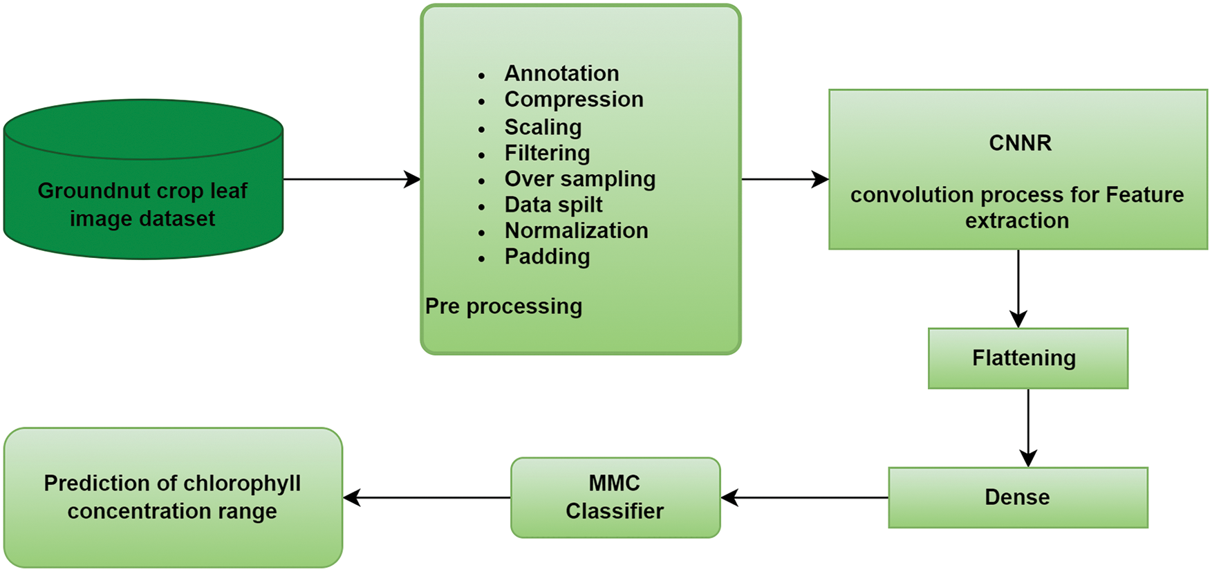
Figure 1: Workflow of SDNP system

Different image processing techniques were applied to the groundnut leaf dataset to obtain the dataset in the required format. Consequently, the preprocessed data is given to the convolution process for extracting the rich source features from the groundnut leaf dataset. Then the extracted features are given to flatten the layer to reduce the dimension of the input. After that, the flattened features are given to the fully connected layer as input for the MMC model for classifying the CC range of groundnut crops.

3.1 Data Collection and Annotation

Leaf images of groundnut crop were collected using an RGB camera in Sivagangai district, Tamil Nadu, to implement the SDNP system. Instantly, the captured leaves' chlorophyll level is measured using an atLEAF chlorophyll metre (FT Green LLC, US). The data collection step-by-step process is shown in Fig. 2.

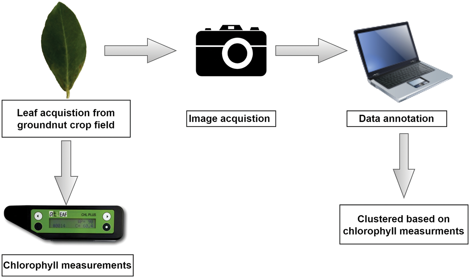
Figure 2: Data collection and annotation

The acquired images fn(x,y) are classified into three classes based on chlorophyll metre measurements: fll(x,y), fbsll(x,y), and fal(x,y). fll-Low level (LL) ranges from 20 to 30, fbsll-beginning stage of low level (BSLL) ranges from 30 to 40, and fal-appropriate level (AL) ranges from 40 to 60 respectively. The total number of collected images is 573, of which 59 images from LL, 115 images from BSLL, and 399 images from AL. The data collection step-by-step process is shown in Fig. 2.

3.2 GLIP-Groundnut Leaf Image Pre-processing

GLIP is necessary to preprocess the groundnut leaf image (fn(x, y)) before running the model. It helps to check for inconsistencies present in fn(x,y) and procure the dataset in the required format [18]. Image annotation has been done on the entire groundnut dataset. Initially, the raw dataset size was 1164.6 MB with a 2352 × 4160 dimension. In the first step of preprocessing, image compression is carried out in a lossless way using Huffman [19] coding to reduce the size of the dataset and storage space, which helps to decrease the processing time. The Compression ratio (CR) is mathematically defined as follows:

CR=ICI0 (1)

IC denotes the dimension of the compressed image and Io denotes the dimension of the original image. Then image downscaling is performed to reduce the dimension of all images in the same dimension. The scale factor (SF) is defined as follows:

SF=ISIDILID (2)

ISID denotes a scaled-down image dimension and ILID denotes IC dimension. After compression and scaling, the entire dataset’s reduced size is 19.074 MB and its dimension is 235 × 416, respectively.

The dataset was collected during the daytime from the crop field. There is a chance of impulse noise occurrence in the original image due to environmental factors. It may damage or change the texture and colour of the images, which are important at the time of feature extraction. Applying a filtering technique can be a solution to avoid these issues. Hence, a median filter [20] is applied to the entire dataset to eliminate the impulse noise from the images. The mathematical expression of the median filter is defined in Eq. (3).

median(s,t)∈Sxy{g(s,t)} (3)

where g(s, t) represents the compressed and scaled-down image and Sxy denotes the rectangular sub-image with the window size m×n which is centred at x,y . To check the quality of original and preprocessed images, the Peak signal-to-noise ratio (PSNR) value is measured for some images. Mainly, the higher PSNR value provides high image quality of the reconstructed image. The PSNR is expressed in decibels (dB) and is calculated as follows:

MSE=1mn∑x=0m−1⁡∑y=0n−1⁡[f(x,y)−K′(x,y)]2 (4)

20log10(max(k(x,y))MSE) (5)

RS=1.0/255.0 (6)

PSNR is defined by MSE (Mean square error) which is denoted in Eqs. (4) and (5). Where m and n represent the image dimensions, x and y denote the index of a specific row and column, f(X,Y) represents the captured image and k′(x,y) represents the degraded image. Next, oversampling, also known as data augmentation is used to increase the size of the dataset, so that it can learn with more features at the time of the training phase. The different augmentation techniques used are rotation, shift, height, shear, zoom, flip, and nearest. Then cross-validation is applied to analyse and fix the data split ratio. Finally, data normalisation is applied to each image to transform the pixel value from 0 to 1. The data normalisation equation is mentioned in Eq. (6).

3.3 CNNR for Feature Extraction

In digital image processing, the Convolution operation combines images and filters to highlight certain important features. In the first step, padding operation is done on pre-processed images to avoid shrinkage which leads to data loss on convolution outputs. Padding process joins pixels around the input images, which increases the images’ size. Two ways of filling Pixel values around images are zero padding and apply neighbour pixel value padding. The zero padding technique utilized in this work with padding value 1. Number of rows and columns are added around the images based on the padding value. Subsequently, a convolution operation is performed in the first layer to obtain the convolution outputs. With its fixed size kernels also known as filters applied on padded images to analyse features. To instruct the kernels’ position and direction on images, stride techniques is used. Each kernel’s weights are filled by using He weight initialization technique which calculates random number with Gaussian probability distribution. Then the outputs are given to activation function. It has two types such as linear and non-linear.

For multidimensional data non-linear activation function is suitable, which helps to obtain feature maps from convolution outputs, after reducing the computational complexity by transforming the pixel values based on certain conditions and learned complex features by introducing nonlinearity. Then in the fourth step, max-pooling kernels were applied on feature maps to get high contrast features, through which the dimension of images got reduced. Max-pooling kernels Weights initialized using He weight initialization technique. The sixth step, the feature maps with prominent features (pooled feature maps) are given to the next layer as input to proceed with the above-mentioned steps. Afterward, the extracted multi-dimensional features flattened as a single long linear vector. Those flattened features are given to a fully connected layer (hidden layer 1). Then those features have given to MMC classification technique with a kernel trick for classifying the chlorophyll concentration range. To obtain the generalized model kernel trick method utilized. This method transforms data from high dimensional space to low dimensional space. Three different kernel tricks such as sigmoid, polynomial and radial basis function [21] are analysed and compared. Among them polynomial kernel selected because of its best performance. The architecture of CNNR-MMC model is shown in Fig. 3.

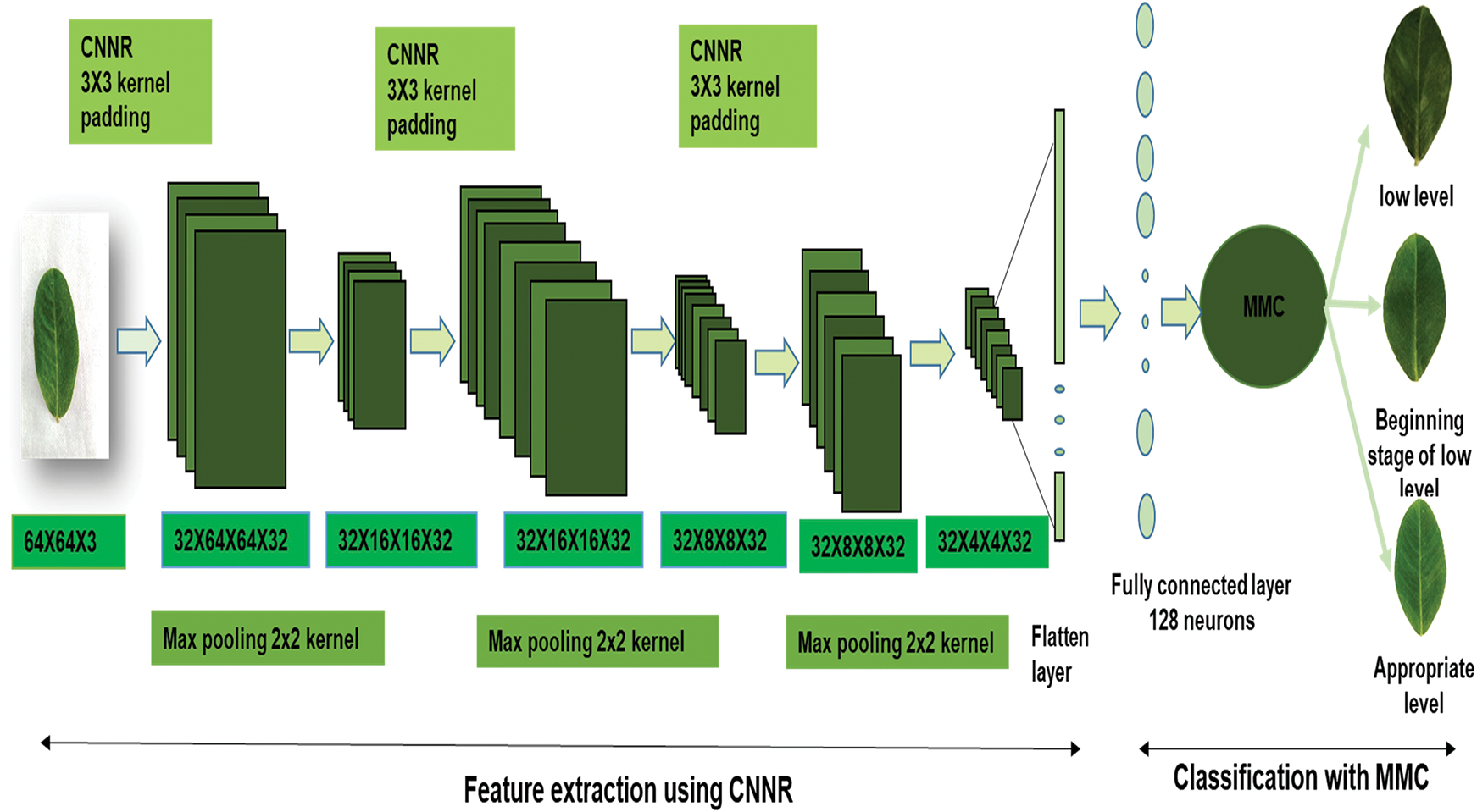
Figure 3: Architecture of CNNR -MMC

While using CNN for feature extraction, the convolution operation with the padding (P) equation is defined in Eq. (7). Then the convolution process outputs (CPO), also known as feature maps, are given to the activation function f (CPO). The major role of the activation function is to squash the real number into fixed intervals. The existing activation functions are sigmoid, tanh, and ReLU, etc., the sigmoid derivative range is 0 to 0.25, which transforms the CPO between 0 to 1. tanh derivative range is 0 to 1, which transforms the CPO between −1 to 1. ReLU transforms the negative value to 0 and keeps the positive value the same. However, these functions face issues such as the vanishing gradient problem, the dead neuron problem, and the leaky relu problem.

Vanishing gradient problem occurs during the back propagation process. It represents the very negligible updated weights. For this reason, multi-layered networks (more than three layers) were not developed two decades ago.

[[nin+2p−fs+1]],[nin+2p−fs+1],Ncf (7)

nout-output feature map, nin-input matrix features, f-kernel size, s-strides

While using ReLU, if one of the derivative values is negative, then it will become zero, and then the updated weight will be equal to the old weight. It represents the dead activation issue. While using leaky ReLU, this issue can be solved, but again it faces a vanishing gradient problem.

To overcome these drawbacks, a novel activation function proposed here is Non-negative Rectified Linear Unit (NNR). It has potential of learning complex patterns and solves the vanishing gradient problem. If the derivative values are positive or greater than 0, it keeps that as same. If the derivative values are negative or less than zero, it converts them to positive values and multiplies them by the fixed learning rate ( η=0.01 ) and n is fixed as constant in the proposed NNR, which can be expressed as follows:

f(CPO)={η×x−n×xCPO=−veCPO=CPOCPO=+ve (8)

Then, the extracted features are flattened to insert them into a dense layer which has M1 to Mn neurons belonging to an M number of neurons. Those features have been provided by M to perform classification.

3.4 Maximum Margin Classification (MMC)

MMC is a machine learning classification algorithm that classifies the training data (input features) with the help of support vectors and marginal planes. These support vectors pass through marginal planes that exist on both sides of the hyperplane at the same distance. If the features are linearly separable, then with the help of hard margin, a hyperplane is generated. Here, it is non-linear separable features. The extracted Positive and negative features are separated using a soft margin to generate a hyperplane with a miss classification ratio. The distance between support vectors is calculated while subtracting the marginal planes (yi). That marginal plane equation is denoted as follows:

wTx+b=+1 (9)

wTx+b=−1 (10)

yi belongs to −1 and +1

wT∥w∥(x2−x1)=2∥w∥ (11)

The distance of the marginal needs to be maximized with the mentioned condition as shown in Eq. (12).

(w∗,b∗)max2∥w∥or(w∗,b∗)min∥w∥2

yi∗wTxi+bi≥1 (12)

The miss classification ratio is measured using the L2 regularisation parameter (total number of miss classifications) when it is multiplied by the summation of error values. Finally, the cost function is calculated using the squared hinge loss function. The cost function expression is denoted as follows:

L(y,y^)=∑i=1b⁡((max(0,1−yi.yi^))2) (13)

b denoted as batch size, yandy^ represent the actual and predicted value respectively.

To reduce the loss ratio, the used optimizer is mini-batch Stochastic Gradient Descent (SGD). It takes a fixed number of records (K) for each epoch, and its resource utility is less when compared to SGD. It reduces the loss ratio, concerning the filters’ pixel value. Depending on the loss ratio, the convolution Filters’ values and max-pooling filters’ values will be updated during back propagation to proceed further until it reaches the global minima.

Wt+1=Wt−η1n∑xεB⁡∇l(x,Wt) (14)

Wt represents the originated weight value and B denotes the fixed batch size, which is a subset of the total number of leaf samples (x). The Number of iterations in each epoch is derived by dividing the total number of records by batch size.

Then the classification performance of the proposed model is evaluated with performance metrics such as Positive predicted value (Ppv), True positive rate (Tpr), and F1 score (F1s).

Ppv=TpTp+Fp (15)

Tpr=TpTp+Fn (16)

F1s=2∗Ppv∗TprPpv+Tpr (17)

Tp-true positive, it indicates the correctly categorised groundnut leaf samples in all three classes. Fp-False positive, it denotes the total number of miss-categorised groundnut leaf samples of the predicted class. Fn-False negative describes the total number of miss classified groundnut leaf samples of true class.

Mpr=TprTpr+12(Fp+Fn) (18)

Mavg=∑i=0i−1⁡F1si (19)

Wavg=∑i=0i−1⁡∑j=0j−1⁡F1si∗Sj (20)

The equalised performance of all leaf samples, all classes and specific classes is calculated using averaging methods such as micro precision (Mpr), micro average (Mavg), and weighted average (Wavg). In Mpr CC range of groundnut, leaf samples are equally contributed to finding the final averaged metric, In the Mavg CC range of groundnut leaf classes are equally contributed to finding the final averaged metric. The Wavg contribution is averaged by the number of leaf samples in each class.

4  Result and Discussion

The CNNR-MMC model implemented experiments were performed in the TensorFlow platform and executed on a system with configuration as developed using Geforce GTX Super_16 GB, Cuda_core_2048 per GPU-1 GHz and clock speed 1 GHz. As discussed in Section 3.1 groundnut dataset in each class is not distributed equally, it is skewed towards the AL class. Initially, the CNNR-MMC model is trained with that imbalanced dataset and analysed the results. The model contains 3 convolution layers, flattened layer and a fully connected layer with 128 neurons. Each convolution layer has 32 convolution filters with kernel size 3 × 3 and max-pooling filter with pool size 2 × 2 and strides 2. The input image dimension is 64 × 64 × 3, 3 represents the depth of the image with red green, and blue colours. The fixed train spilt ratio is 80:20. The used activation function in the convolution layers and dense layer is NNR and in the classification process MMC technique with L2 regularization. The fixed regularization learning parameter is 0.01. The utilized optimizer is SGD with a learning rate of 0.3. During feature extraction the extracted parameter in the first convolution layer is 896, the second convolutional layer is 9248, and in the third convolutional layer is 9248. The extracted parameters from the dense and classification layer are 66,051. The total number of the extracted parameter using CNNR-MMC is 85,443. It provides zero non-trainable parameters.

As shown in Figs. 4a and 4b, with an imbalanced dataset, the model’s obtained training accuracy and loss are 0.83% and 0.84%, respectively, and the validation accuracy and loss are 0.73% and 1.03%, respectively, in the 100th epoch.

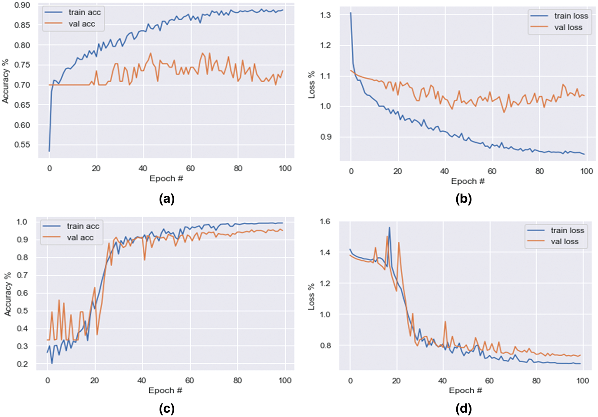
Figure 4: Graph of CNNR-MMC model’s accuracy and loss. Imbalanced dataset-(a) training accuracy and validation accuracy, (b) training loss and validation loss. Balanced dataset-(c) training accuracy and validation accuracy, (d) training loss and validation loss

Based on the loss observations as shown in Table 1 with the imbalanced dataset, and inconsistent predictions as shown in Figs. 5a and 5b, the model has high variance and low bias. Hence, it implies that which comes under the overfitting problem.

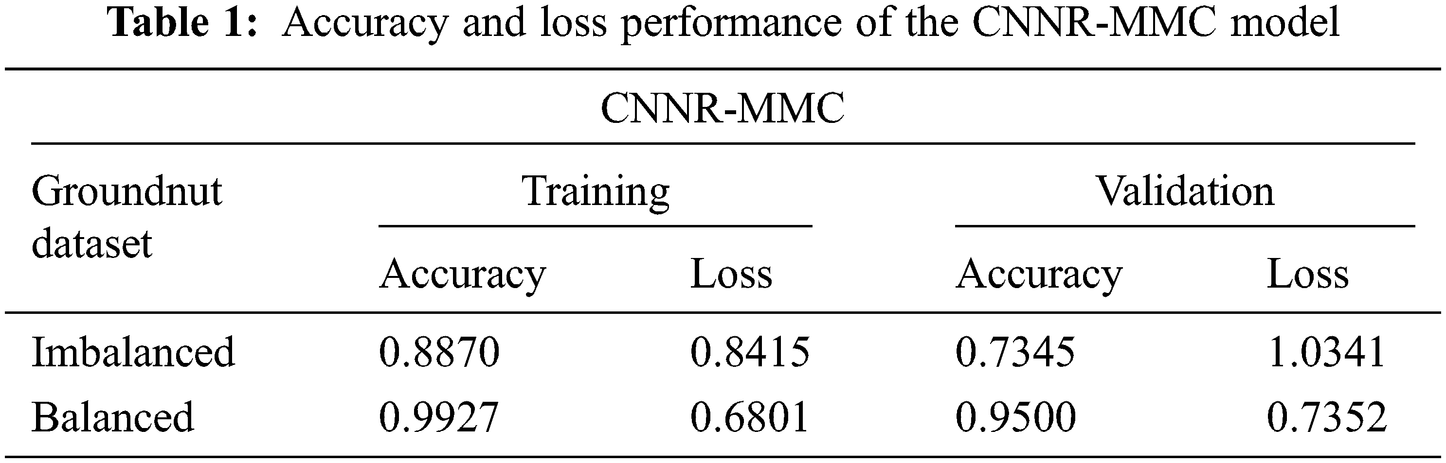
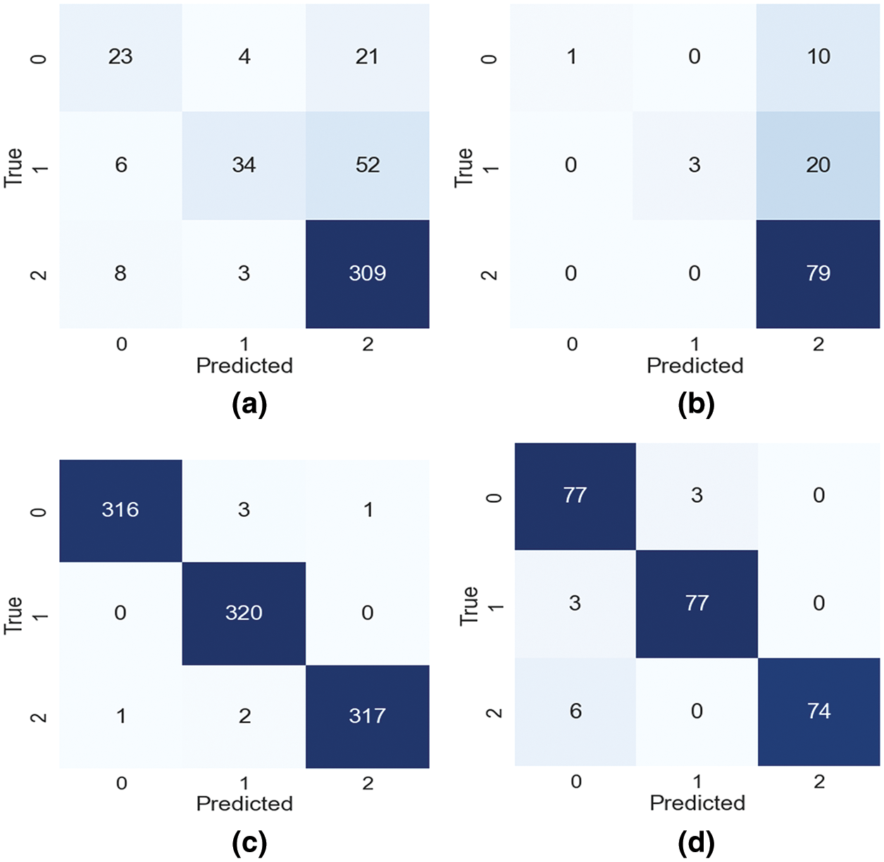
Figure 5: Confusion matrix of CNNR-MMC model. Imbalanced dataset-(a) training, (b) validation. Balanced dataset-(c) training, (d) validation

The augmentation technique is applied to all three classes to balance the dataset, and balance the observed reducible error (bias and variance). The increased number of samples in the LL, BSLL and AL classes is 341, 285, and 1 respectively. After augmentation, the total number of samples is 1200. While training the CMPO-NNSR-MMC model with the balanced dataset, as shown in Figs. 4c and 4d, the model achieved training and validation accuracies of 0.99% and 0.95%, respectively, in the 100th epoch. Figs. 5c and 5d show the confusion matrix with true positive samples and miss-classified samples of each class.

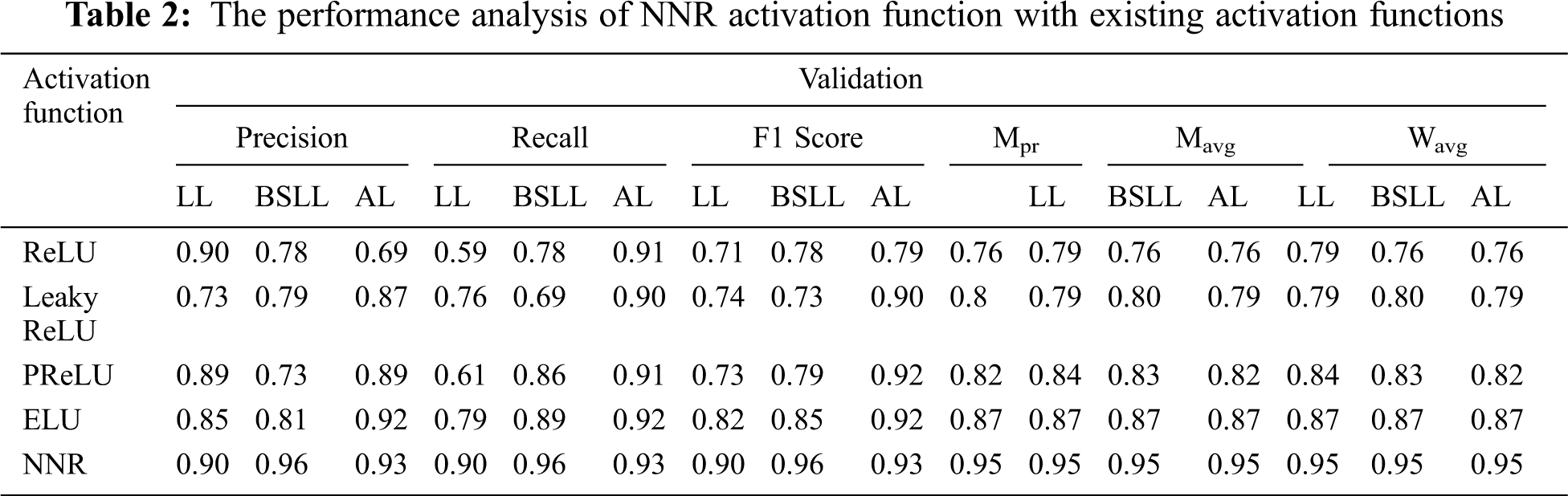
The loss percentage of training is 0.68% and validation is 0.73%. As shown in the Table 1 after augmentation, the loss percentage reduced from 0.84% to 0.68% and 1.03% to 0.73% during training and validation, respectively. Therefore, with the imbalanced dataset, the model prediction is consistent, low- bias, and well balanced. To know the performance of the NNR activation function in the CNNR-MMC model, it is analysed and compared with existing activation functions including ReLU, Leaky ReLU, PReLU (parametric relu), and ELU (exponential linear unit) using precision, recall, and f1 score. The obtained results show that the proposed model with the NNR activation function provided better results when compared to other activation functions, as shown in Table 2.

The proposed model’s performance on the groundnut dataset was compared to that of pretrained imagenet models with depths of 16, 19, 55, 81, 103, and 105, respectively, from the VGG 16 and VGG 19 by Simonyan et al. [22], MobileNet by Google researchers [23], Xception by Francois Chollet [24], ResNet50V2 He et al. [25], and MobileNetV2 [23]. These models alone are selected for comparison analysis, because of their less complex structure compared to other pre-trained deep CNN models with different versions. These models are well trained using the ImageNet dataset with over 1000 categories. A transfer learning approach is applied to each model by changing the output layer with three classes. In this work, the groundnut dataset with three categories is trained using those ImageNet models with pre-trained weights. All the pre-trained models obtained good accuracy in the 100th epoch, as shown in Table 3. While observing the error ratio during training and validation of each model, it shows high variance. The graphical visualisation of all the pre-trained models’ output for training and validation is shown in Fig. 6.

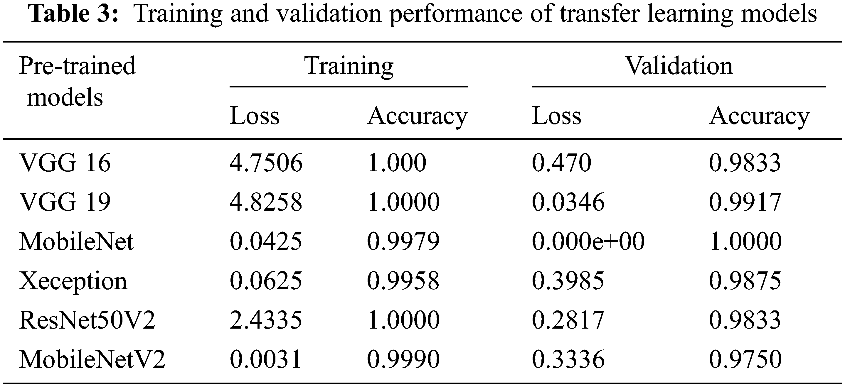
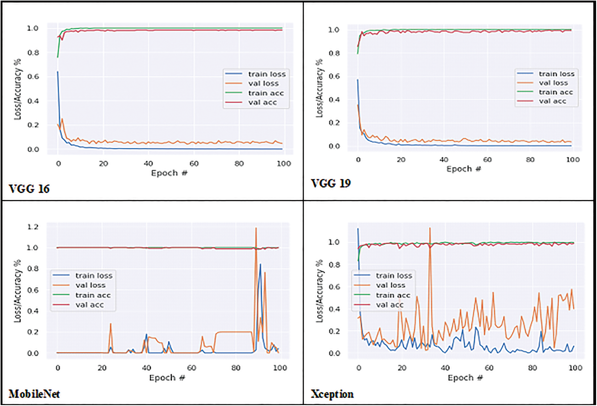
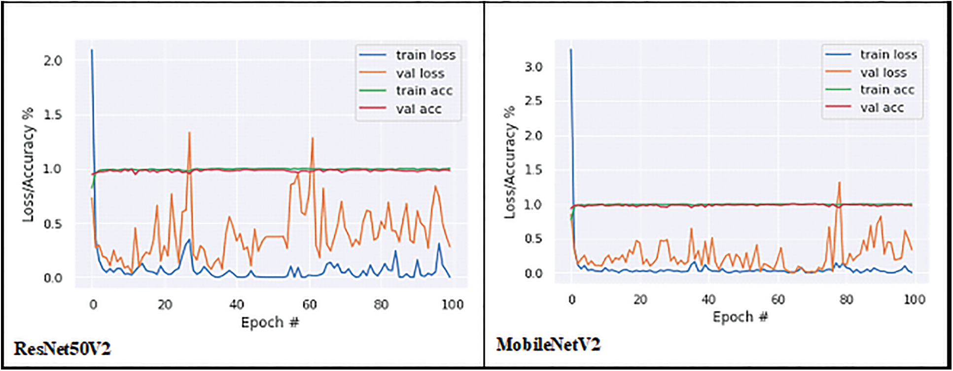
Figure 6: Training and validation graph of transfer learning models

Therefore, to visualise the actual and predicted classification ratio in each class confusion matrix as shown in Fig. 7, which clearly shows the missclassified samples of all models in each class.

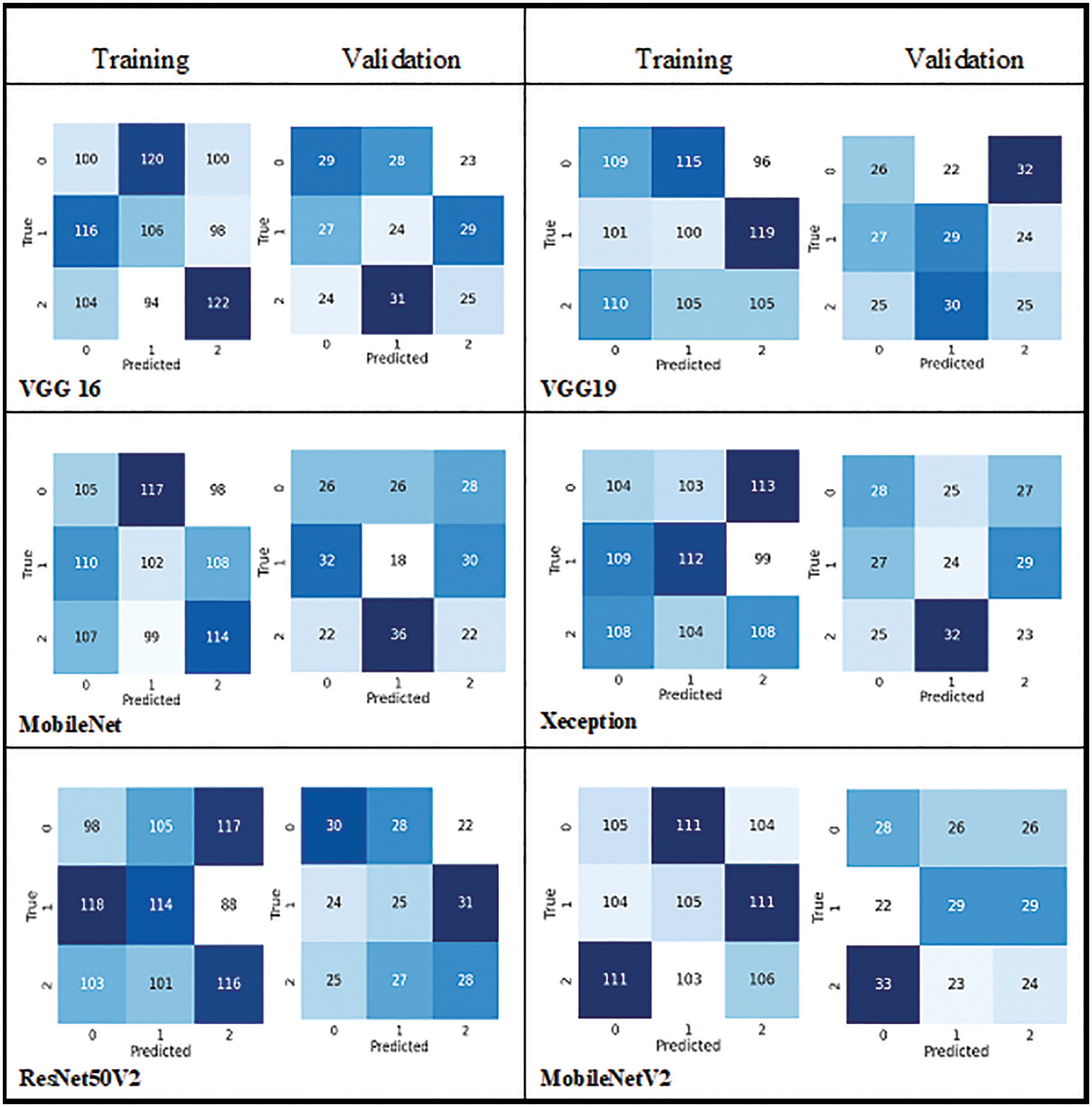
Figure 7: Confusion matrix of all pre-trained models

Accuracy alone will not be an accurate measure when the models’ results show high variance. Apart from accuracy, other performance metrics are calculated such as precision, recall, F1 score, micro-precision, macro average, and weighted average. These performance metrics results are very low and range from 0.28% to 0.38% in all pre-trained models, as they have more miss-classification samples in the confusion matrix. But with the CNNR-MMC model, better results ranged from 0.90% to 0.95%. It implies that though the selected pre-trained models are less complex compared to other pre-trained models, they have not performed well to predict chlorophyll concentration of groundnut leaf images with smaller dataset, and all models faced overfitting problems.

While observing the number of trainable parameters in each model, it varied as each model has a different depth. The extracted trainable parameter count is shown in Table 4, though the VGG models’ parameters are less when compared to the CNNR-MMC model, they do not perform well and show a high variance in loss ratio during training and validation.

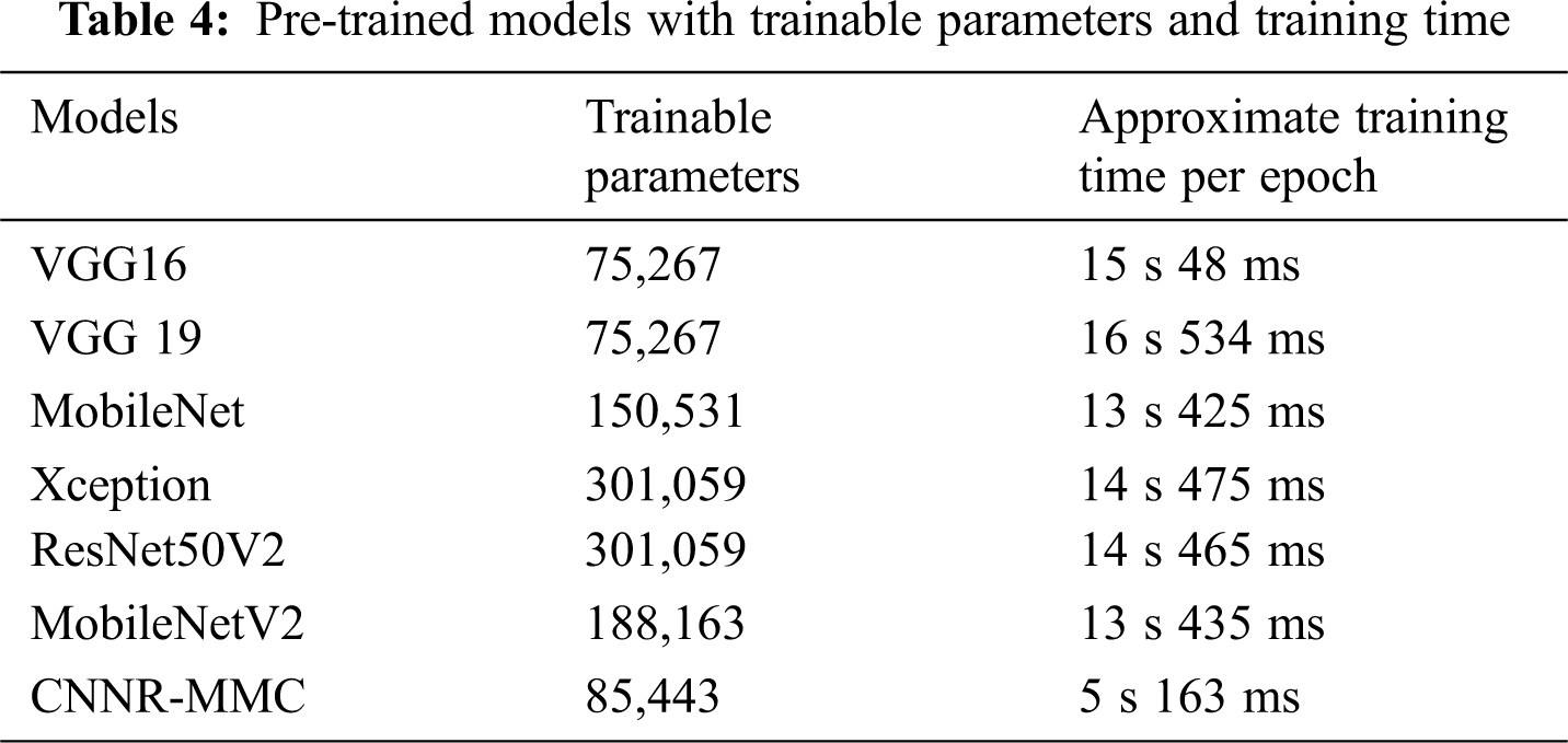
Then training time for all models is noticed. However, MobileNet and Inception have more layers, when compared to the VGG model, but both take less time for training. But compared to all models, CNNR-MMC takes less training time.

As shown in Table 5, the CNNR-MMC model achieved high accuracy when compared with existing literature work.

5  Conclusion

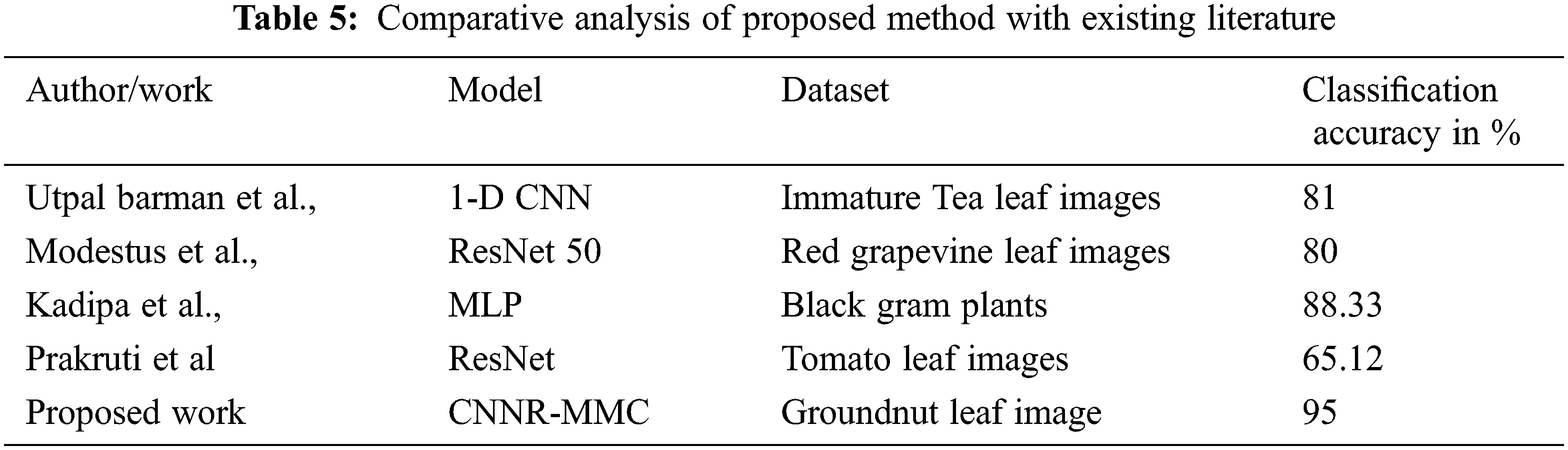
Chlorophyll deficiency represents a major constraint for groundnut crop production, it could not be identified before visible symptoms, particularly in the early stage. Therefore, the CNNR-MMC model is implemented to identify and classify the CC range of groundnut crops. The GLIP performed before deploying the dataset into the model reduced the processing time, provides enhanced feature extraction, and will help further improve the model’s classification performance. The same dataset is trained and evaluated with different transfer learning models. The attained result shows that the CNNR-MMC outperformed well and obtained the highest accuracy with less training time while comparing to ImageNet pre-trained models. The achieved CNNR-MMC model’s training accuracy and validation accuracy are 99% and 95% respectively. This scalable and cost-effective SNDP system can be adopted by all types of farmers to predict the CC range of groundnut crops in a real-time field. In the future work, the model will be improved to predict other macro and micro nutrients with a fertiliser recommendation system.

Funding Statement: The authors received no specific funding for this study.

Conflicts of Interest: The authors declare that they have no conflicts of interest to report regarding the present study.

References

1. J. Cohan, C. Le Souder, C. Guicherd, J. Lorgeou, P. Du Cheyron et al., “Combining breeding traits and agronomic indicators to characterize the impact of cultivar on the nitrogen use efficiency of bread wheat,” Field Crops Research, vol. 242, no. 9, pp. 107588, 2019. [Google Scholar]
2. F. N. Kogan, “Remote sensing of weather impacts on vegetation in non-homogeneous areas,” International Journal of Remote Sensing, vol. 11, no. 8, pp. 1405–1419, 1990. [Google Scholar]
3. W. Li, Z. Niu, C. Wang, W. Huang, H. Chen et al., “Combined use of airborne LiDAR and satellite GF-1 data to estimate leaf area index, height, and aboveground biomass of maize during peak growing season,” IEEE Journal of Selected Topics in Applied Earth Observations and Remote Sensing, vol. 8, no. 9, pp. 4489–4501, 2015. [Google Scholar]
4. M. Kerkech, A. Hafiane and R. Canals, “Vine disease detection in UAV multispectral images using optimized image registration and deep learning segmentation approach,” Computers and Electronics in Agriculture, vol. 174, no. 5, pp. 105446, 2020. [Google Scholar]
5. Y. Wang, D. Wang, G. Zhang and J. Wang, “Estimating nitrogen status of rice using the image segmentation of G-R thresholding method,” Field Crops Research, vol. 149, no. 8, pp. 33–39, 2013. [Google Scholar]
6. Z. Xu, X. Guo, A. Zhu, X. He, X. Zhao et al., “Using deep convolutional neural networks for image-based diagnosis of nutrient deficiencies in rice,” Computational Intelligence and Neuroscience, vol. 2020, no. 8, pp. 1–12, 2020. [Google Scholar]
7. P. Bhatt, S. Sarangi and S. Pappula, “Comparison of CNN models for application in crop health assessment with participatory sensing,” in Global Humanitarian Technology Conf., San Jose, CA, USA, pp. 1–7, 2017. [Google Scholar]
8. U. Barman, “Deep convolutional neural network (CNN) in tea leaf chlorophyll estimation: A new direction of modern tea farming in Assam, India,” Journal of Applied and Natural Science, vol. 13, no. 3, pp. 1059–1064, 2021. [Google Scholar]
9. S. Yadav, Y. Ibaraki and S. Gupta, “Estimation of the chlorophyll content of micro propagated potato plants using RGB based image analysis,” Plant Cell, Tissue and Organ Culture, vol. 100, no. 2, pp. 183–188, 2010. [Google Scholar]
10. U. Ukacgbu, L. Tartibu, T. Laseinde, M. Okwu and I. Olayode, “A deep learning algorithm for detection of potassium deficiency in a red grapevine and spraying actuation using a raspberry pi3,” in Int. Conf. on Artificial Intelligence, Big data, Computing and Data Communication Systems, Durban, South Africa, pp. 1–6, 2020. [Google Scholar]
11. K. A. Myo Han and U. Watchareeruetai, “Blackgram plant nutrient deficiency classification in combined images using convolutional neural network,” in Int. Electrical Engineering Congress, Chiang Mai, Thailand, pp. 1–4, 2020. [Google Scholar]
12. Z. Qiu, F. Ma, Z. Li, X. Xu, H. Ge et al., “Estimation of nitrogen nutrition index in rice from UAV RGB images coupled with machine learning algorithms,” Computers and Electronics in Agriculture, vol. 189, no. 8, pp. 106421, 2021. [Google Scholar]
13. O. Hassanijalilian, C. Igathinathane, C. Doetkott, S. Bajwa, J. Nowatzki et al., “Chlorophyll estimation in soybean leaves infield with smartphone digital imaging and machine learning,” Computers and Electronics in Agriculture, vol. 174, pp. 105433, 2020. [Google Scholar]
14. S. Azimi, T. Kaur and T. K. Gandhi, “A deep learning approach to measure stress level in plants due to nitrogen deficiency,” Measurement, vol. 173, no. 15, pp. 108650, 2021. [Google Scholar]
15. A. Amirruddin, F. Muharam, M. Ismail, M. Ismail, N. Tan et al., “Hyperspectral remote sensing for assessment of chlorophyll sufficiency levels in mature oil palm (Elaeis guineensis) based on frond numbers: Analysis of decision tree and random forest,” Computers and Electronics in Agriculture, vol. 169, pp. 105221, 2020. [Google Scholar]
16. S. Bhadra, V. Sagan, M. Maimaitijiang, M. Maimaitiyiming, M. Newcomb et al., “Quantifying leaf chlorophyll concentration of sorghum from hyperspectral data using derivative calculus and machine learning,” Remote Sensing, vol. 12, no. 13, pp. 2082, 2020. [Google Scholar]
17. A. Mahajan, N. Sharma, S. Aparicio Obregon, H. Alyami, A. Alharbi et al., “A novel stacking-based deterministic ensemble model for infectious disease prediction,” Mathematics, vol. 10, no. 10, pp. 1714, 2022. [Google Scholar]
18. S. Khurana, G. Sharma, N. Miglani, A. Singh, A. Alharbi et al., “An intelligent fine-tuned forecasting technique for COVID-19 prediction using neuralprophet model,” Computers, Materials & Continua, vol. 71, no. 1, pp. 629–649, 2022. [Google Scholar]
19. S. Singh and V. Gupta, “JPEG image compression and decompression by Huffman coding,” International Journal of Innovative Science and Research Technology, vol. 1, no. 5, pp. 8–14, 2016. [Google Scholar]
20. K. Boateng, B. Asubam and D. Blaar, “Improving the effectiveness of the median filter,” International Journal of Electronics and Communication Engineering, vol. 5, no. 1, pp. 85–87, 2012. [Google Scholar]
21. H. Sun and R. Grishman, “Lexicalized dependency paths based supervised learning for relation extraction,” Computer Systems Science and Engineering, vol. 43, no. 3, pp. 861–870, 2022. [Google Scholar]
22. K. Simonyan and A. Zisserman, “Very deep convolutional networks for large-scale image recognition,” arXiv preprint arXiv: 1409.1556, pp. 1–14, 2014. [Google Scholar]
23. A. G. Haward, M. Zhu, B. Chen, D. Kalenchenko, W. Wang et al., “MobileNets: Efficient Convolutional neural networks for mobile vision applications,” ArXiv, vol. abs/1704.04861, pp. 1–9, 2017. [Google Scholar]
24. F. Chollet, “Xception: Deep learning with depthwise separable convolutions,” in Conf. on Computer Vision and Pattern Recognition, Honolulu, HI, USA, pp. 1800–1807, 2017. [Google Scholar]
25. K. He, X. Zhang, S. Ren and J. Sun, “Deep residual learning for image recognition,” in Conf. on Computer Vision and Pattern Recognition, Las Vegas, NV, USA, pp. 770–778, 2016. [Google Scholar]
Cite This Article
Copyright © 2023 The Author(s). Published by Tech Science Press.
This work is licensed under a Creative Commons Attribution 4.0 International License , which permits unrestricted use, distribution, and reproduction in any medium, provided the original work is properly cited.
Downloads
Citation Tools