Multi Class Brain Cancer Prediction System Empowered with BRISK Descriptor

1  Introduction

The growth of abnormal cells in the brain is referred as brain tumour or brain cancer. Some tumours are cancerous and others are non-cancerous. Magnetic Resonance Imaging (MRI) images are often used in medical domain for the diagnosis of various diseases. Several machine learning algorithms such as Naive Bayes (NB), Decision Tree (DT), Gaussian, and Support Vector Machine (SVM) along with radial basis function kernel are reviewed in [1] for brain cancer diagnosis. Watershed algorithm is discussed in [2,3] for segmenting the brain tumours from the MRI images. To perform effective training and testing, ten-fold cross validation [1] and five-fold cross validation [4] is used to improve the performances. Recent advances in medical diagnosis especially in disease diagnosis among patients to detect tumor, MRI images are used than other medical imaging modalities.

A brain tumor investigative system is built in [5] using fast Fourier transform. A binary SVM classification (normal/abnormal) is employed for the classification using the reduced features by minimal-redundancy-maximal-relevance algorithm. A hybrid algorithm is employed in [6] which comprises of SVM, genetic algorithm and Principle Component Analysis (PCA). Spatial gray level dependence approach is used for mining the relevant features of abnormal as well as normal patterns. In addition, different machine algorithms are used in [7–10] in detecting brain tumors.

Automatic brain tumour detection is analyzed in [11] using Random Forest (RF) and binary decision tree algorithms. It uses the local information of each voxel from the multispectral volumetric MRI images. Texture features are extracted from the co-occurrence matrix for brain tumour classification in [12]. Anisotropic diffused MRI brain image is enhanced by using histogram equalization before extracting features from the segmented images. For segmentation, Chan-Vese active contour model is employed.

The whole image around the skull is used for the classification in [13]. It uses NB, DT, and Neural Network (NN) for the classification. Brain image classification using NN with single hidden layer is described in [14]. It uses adaptive median filter for preprocessing the MRI brain image and k-means clustering is used for the segmentation. Features such as contrast, energy, correlation and homogeneity are extracted from the segmented image for the classification. The same set of features in [14] is utilized for MRI brain cancer classification using a multi-layer perceptron and RF classifier in [15]. Wavelet based system is discussed in [16] for classifying brain tumours into high grade or low grade. At first, the brain tumour region is detected using k-means clustering and then wavelet and PCA based features are extracted. Finally, SVM is used for binary classification. Though different deep learning architectures [17–19] are developed for MRI brain image classification system, they suffer from high computation time, memory and also fine tuning of parameters is very difficult. The contribution of this research work is as follows:

•   Developing an efficient Binary Robust Invariant Scalable Keypoints (BRISK) descriptor tool that describes the key points in the MRI brain image to point out the affected region.

•   Additional specific image features are extracted and utilized to further improve the system’s performances.

•   Applying multi-class classifier to categorize the images into normal or one of the abnormalities such as glioma, meningioma, and pituitary.

The main objective is to develop machine learning algorithms such as k-Nearest Neighbour (kNN), SVM and RF for multi-class classification of MRI brain images. The organization of the paper is as follows: Section 2 discusses the proposed features such as BRISK and image based features along with the mathematical backgrounds of the machine learning algorithms. Section 3 discusses the multi-class classification results obtained by the proposed Multi-Class Classification (MCC) system using 3264 MRI brain images. The last section provides the conclusions arrived from the outcomes of the proposed MCC system for MRI brain image classification.

2  Methods and Materials

In this section, the proposed MCC system for classifying the MRI images into four classes such as normal, glioma, meningioma, pituitary using machine learning classifiers is discussed. The workflow of the proposed MCC system is depicted in Fig. 1.

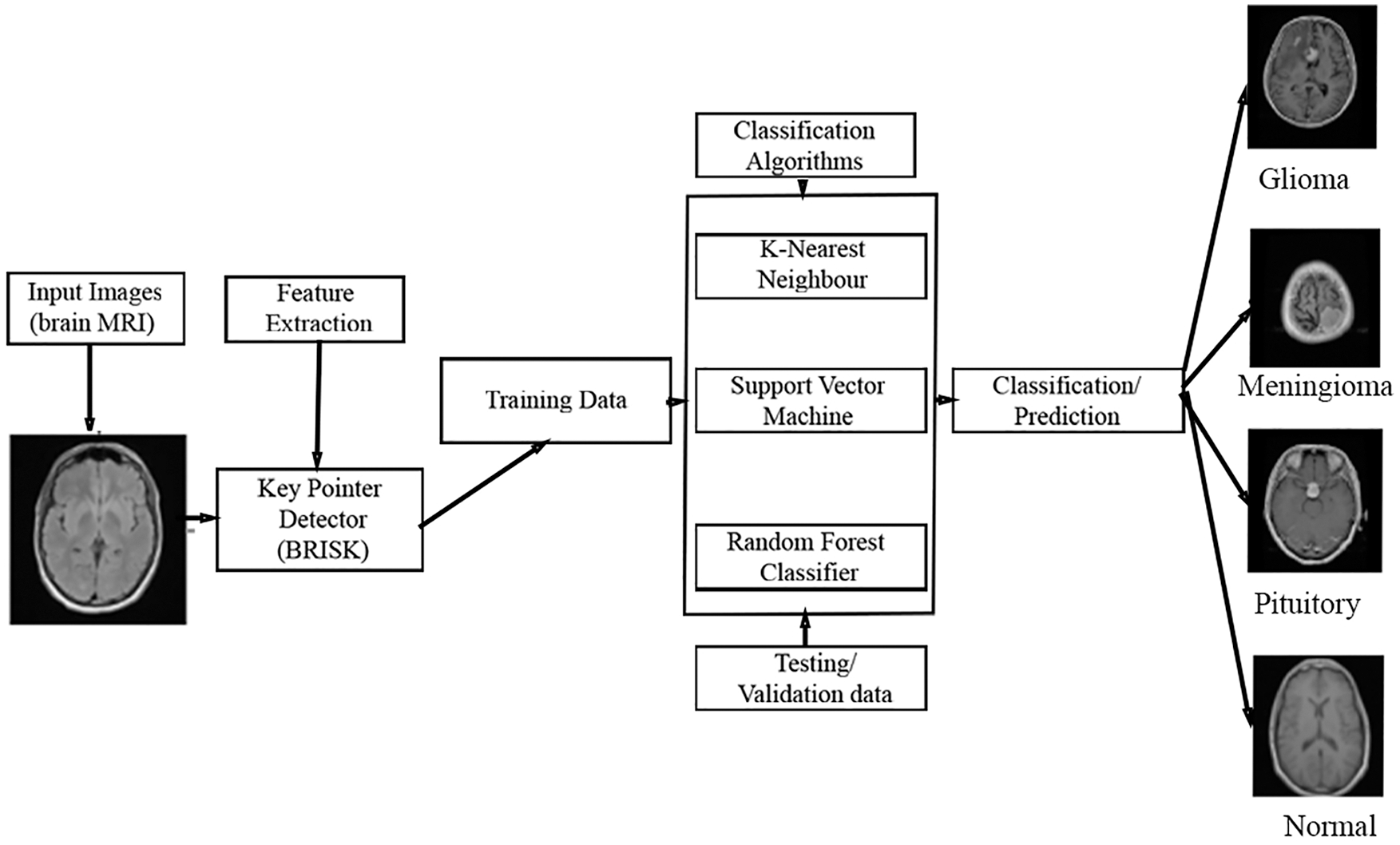
Figure 1: Proposed MCC system for MRI brain image classification

2.1 Brisk Descriptor

Feature extraction is a method utilized to recognize or extract key parameters from input images as initial information to obtain the novel data. In this work, key pointer detection method is applied to detect the features and also locate the extracted features via key points. Especially, BRISK algorithm is utilized which is an attribute point recognition as well as depiction approach with scalable invariance along with turning round. Moreover, this detector contest attributes among two images via tuning the parameters up to 200 values. The group of key points comprises of points cultures image positions linked with floating point scaled principles. The BRISK descriptor is collected as two-fold string through adding the outcomes of effortless intensity of image comparison trials. This intensity comparison helps to enhance the image descriptiveness.

Fig. 2 depicts the BRISK descriptor used for feature extraction. BRISK descriptor is applied in [20] to identify key points, then description and finally undergo matching process. The current descriptor which is used for feature extraction consists of coaxial rings. We should consider little scrap of the coaxial rings and yet to apply Gaussian method for smoothening the brain images while we are taking every point in the circle. The red colour mentioned in the circle represented how long the divergence of filter took place in every point. It captures the group of undersized couples, spins the couples by point of reference evaluated and then creates assessment in the form of Eq. (1).

b={1,I(Pjασj)>I(Piασi);0otherwise (1)

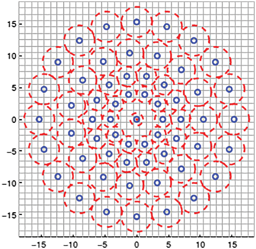
Figure 2: BRISK descriptor used for feature extraction

For every undersized couple, it obtains smoothened intensity of sampling points and then finds whether the first pixel of smoothened intensity is greater than second pixel. If the first pixel is greater than second pixel then the descriptor is considered as one or otherwise 0. Hence this descriptor is suitable for feature extraction on images even in very short pairs.

2.2 Image Features

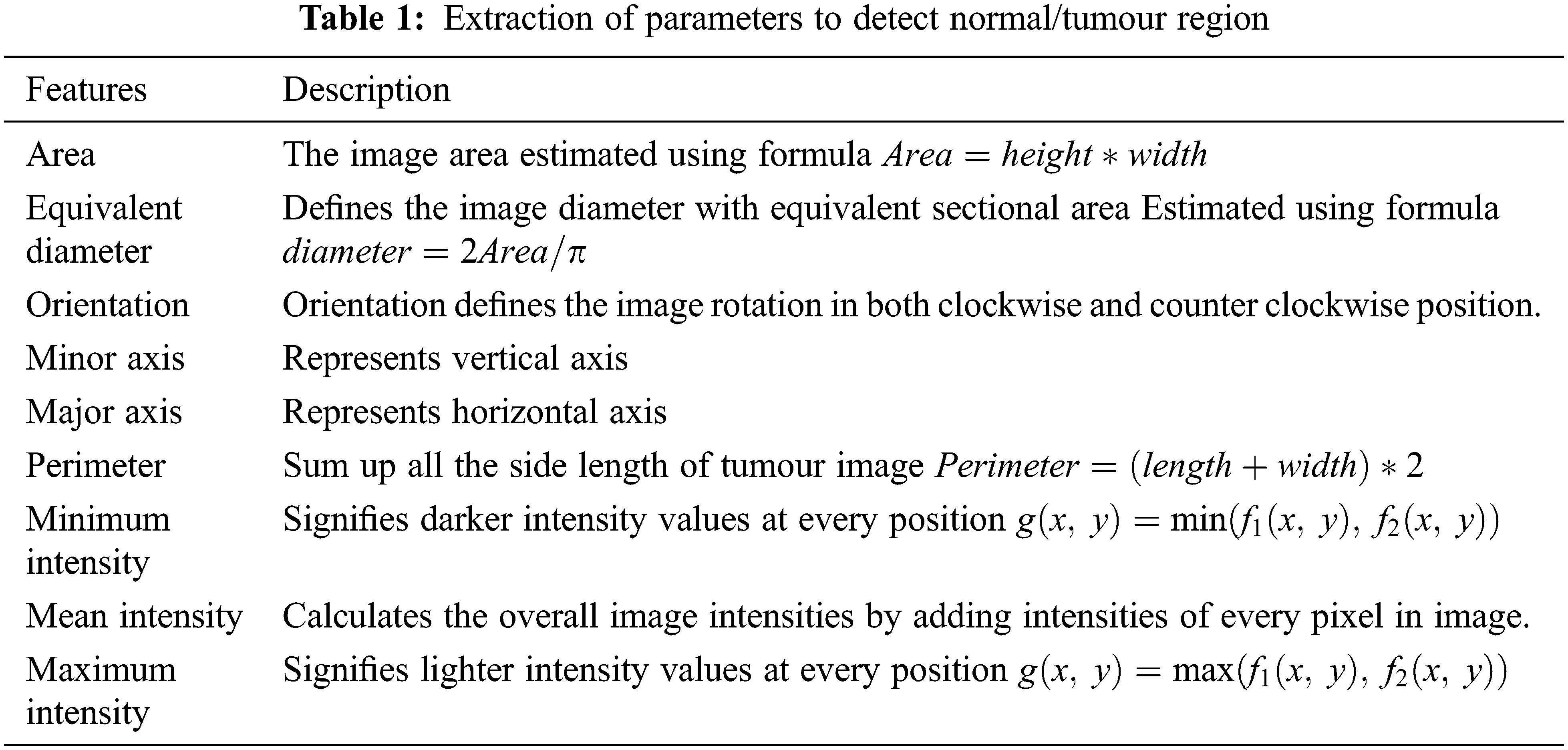
The image features extracted from MRI brain images are image area, equivalent diameter, orientation, minor & minor axis, perimeter, minimum intensity, maximum intensity level and mean intensity level. The features which are extracted from the MRI brain images are described in Tab. 1.

2.3 Classification Algorithms

In this sub-section, three different machine learning algorithms which are used to classify the input MRI brain images into different classes of tumours are discussed.

2.3.1 k-Nearest Neighbour Algorithm

kNN algorithm is one of the supervised machine learning classification algorithms which helps to distinguish the input data into several classified data. In accordance with appropriate distance metric, classifying the input image described as vectors has completed by finding k- closest training vectors of input image. The k value is set to 1. The vectors of an image represented as X which is allocated to one class that has majority of nearest neighbours fit done. Euclidean distance is the important metric for identifying the nearest neighbours by using distance function as well as voting function. The Euclidean distance is computed using the formula mentioned in Eq. (2).

Euclideandistanced(x,y)=∑i=1n(yi−xi)2 (2)

The other distance metrics used in kNN classifier is as follows:

cityblock(x,y)=|x1−y1|+|x2−y2|+⋯|xn−yn| (3)

cosine(x,y)=∑ixiyi∑ixi2∑iyi2 (4)

corr(x,y)=N∑xy−(∑x)(∑y)[N∑x2−(∑x)2][N∑y2−(∑y)2] (5)

All learning algorithms incorporate with both training and testing stages. Hence we have to follow these steps to perform KNN algorithm

(i)    Calculate the appropriate distance metric.

(ii)    During training stage, in accordance with extracted features, accumulate the training images as a duo (D) i.e., D=xi,yi where i = 1, 2, …, n and xi defines the training image from the overall allotted trained image samples yi.

(iii)   Estimate the distance among novel feature vector of an image as well as all training image too during testing stage. Also, this algorithm breeds the nearest data pixels to the unlabeled portion on the images.

(iv)   Finally based on voting the classification of images has done.

2.3.2 Support Vector Machine

SVM is one of the supervised machine learning approaches to perform classification task on images. This method has frequently established to improve the classification results when compared to other pattern identification approaches. The SVM based systems are extremely smart for distinguishing different patterns in the data’s or images. Moreover, SVM method try to establish finest isolating hyper plane among several classes by finding support vectors which are located at the boundary of every hyper plane [21–23]. If N training samples are characterized by [Xi,Yi] where i = 1, 2, 3, …, N and Yi∈[−1,+1]

•   Class 1: Yi  = +1

•   Class 2: Yi  = −1

Here the two classes such as class 1 and class 2 are separated using hyper plane parameters defined by a vector v and bias v0 that isolate the classes with no error described in Eq. (6).

f(x)=v.x+v0=0 (6)

To identify the hyper plane, v and v0 will be evaluated in such a manner that yi(v.xi+v0)≥+1 for Yi = +1 (Class 1) and yi(v.xi+v0)≤−1 for Yi = −1 (Class 2). The combination of these two generates Eq. (7).

yi(v.xi+v0)−1≥0 (7)

Fig. 3 depicts the two-class classification by SVM classifier.

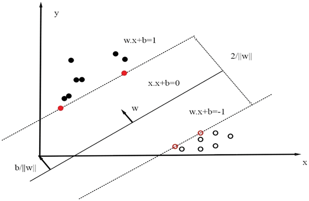
Figure 3: SVM classifier classifies into two classes via hyper planes

The objective of hyper plane is to put down the highest boundary among classes. The vectors related with SVM should mention to detect the optimal hype plane which categorizes the classes. The support vectors reclined on two hyper planes that are matching to best possible one [22], which is given in Eq. (8).

v.xi+vo=±1 (8)

After rescaling of hyper plane parameters v and also v0, the boundary value is described as 2‖v‖ . To attain the optimal hyper plane, the following optimization issues have to be resolved Minimize 12v2 Subject to yi(v.xi+v0)−1≥0fori=0,1,2,…,N . The above issue can be converted in Eq. (9) by means of Lagrangian method

Maximize∑i=1Nλ−12∑i,j=1Nλiλjyiyj(xi.xj) (9)

Subject to ∑i=1N⁡λiyi=0whereλi≥0,i=0,1,2,…,N . Here λi refers to langrangian multipliers. The best hyper plane Discriminant function in this formulation is specified in Eq. (10).

f(x)=∑i∈Sλiyi(xix)+w0 (10)

Here S refers to the split in training images which points non-zero Lagrangian multipliers. Such training images are known as support vector. The cost function which helps to amalgamate the highest boundary as well as lowest error by means of special variables named as δ . Eq. (11) represents the cost function as

costfunction=12||w||2+C∑i=1Nδi (11)

SVM plots the input image represented in vectors (x) into highly dimensional image attributes and in this case, finest isolation of hyper plane is created in that space. Such plotting generates additional complications to the dilemma. The representation of inner product function is defined in Eq. (12).

φ(x)φ(y)=K(x,y) (12)

But K (x, y) represents kernel function. The binary optimization issues can be created as in Eq. (13).

Maximize∑i=1Nλi−12∑i,j=1NλiλjyiyjK(xi.xj) (13)

And finally the consequential classifier becomes

f(x)=∑i∈SλiyiK(xix)+w0 (14)

For object based image investigation, multi label classification is used in [24] for classifying images into several classes using SVM classifier and multi class CNN performed in [25]. Brain tumour is assorted and also multi-class classification is desirable for classifying images into numerous classes such as glioma tumour, meningioma, pituitary and normal. SVM can be applicable for multi-class issues with so called single vs. remaining method (one vs. all). SVM technique trained autonomously among one class as tumour (positive) and the other class will be with no tumour (negative) in case of N issues.

To work with non-linear data, kernel trick is employed. Different kernels such as quadratic, Radial Basis Function (RBF) and polynomial are used in this work with the standard linear kernel. Their definitions are as follows:

RBF(x,y)=exp⁡(‖x−y‖22σ2) (15)

Quadratic(x,y)=1−‖x−y‖2‖x−y‖2+C (16)

Polynomial(x,y)=(αxT.y+C)d (17)

Linear(x,y)=xT.y+K (18)

where σ is the standard deviation and d is the polynomial degree (d = 3). To obtain best and optimal parameters (C, σ ), grid search algorithm is employed with C (from 23 to 2−3) and σ (from 26 to 2−6). The best obtained results are discussed in the next section.

2.3.3 Random Forest

The automated segmentation as well as classification of brain stroke images is discovered using RF classifier that attains highest accuracy in [25]. Forest has numerous (group of) trees. Likewise, the RF algorithm works. RF classifier is one of the classifiers wherein many decision trees are utilized to construct afforest which is depicted in Fig. 4.

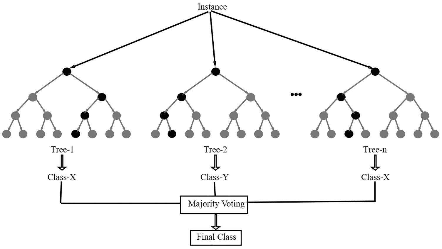
Figure 4: RF classifier

This algorithm is working better while the input dataset is bulky. The forest is highly vigorous while larger quantity of decision trees utilized during decision production procedure. Initially the image dataset is split into two halves with analogous formation. The edge function using RF algorithm is defined as,

mg(X,Y)−αVn.I(hn(X)=Y)−j≠YmaxαVn.I(hn(X)=j) (19)

Here I refer to Indication function h1 (X), h2(X), …, hn(X) are classifiers with ensembling method where X and Y are random vectors. The function that denotes error which is expressed in Eq. (20)

Error=PX,Y(mg(X,Y)<0)ifhn(X)=h(X,Θn) (20)

Now the edge function equation for RF is rewritten in Eq. (21)

mr(X,Y)=PΘ.(h(X,Θ)=Y)−j≠YmaxPΘ.(h(X,Θ)=j) (21)

Here h(X,Θ) represents the potency of classifiers which is represented in Eq. (22)

S=EX,Ymr(X,Y) (22)

The RF method is a time-saving approach that combines numerous decision trees into a single tree for the best prediction accuracy. The step by step procedures for RF algorithm are as follows:

(i)    A novel image is constructed from original given brain MRI image by means of sampling as well as reducing the 1/3 rd portion of row images.

(ii)    Now the algorithm is trained to produce novel images from sample reduction and also evaluates balanced error.

(iii)   At every pixel of the image first column is chosen from total number of columns available.

(iv)   Many decision trees develop concurrently and then ultimate output is predicted through gathering of every decision to attain better accuracy classification.

3  Results and Discussions

3.1 Data Collection

The performances of the proposed MCC system for classifying MRI brain images are assessed using a public database. It is freely downloadable from [26]. The MRI images in this database are collected from healthy and cancer affected patients and having four classes of images such as normal, glioma, meningioma and pituitary. Tab. 2 shows the class distribution of MRI brain images in this database. Fig. 5 shows sample images in each category.

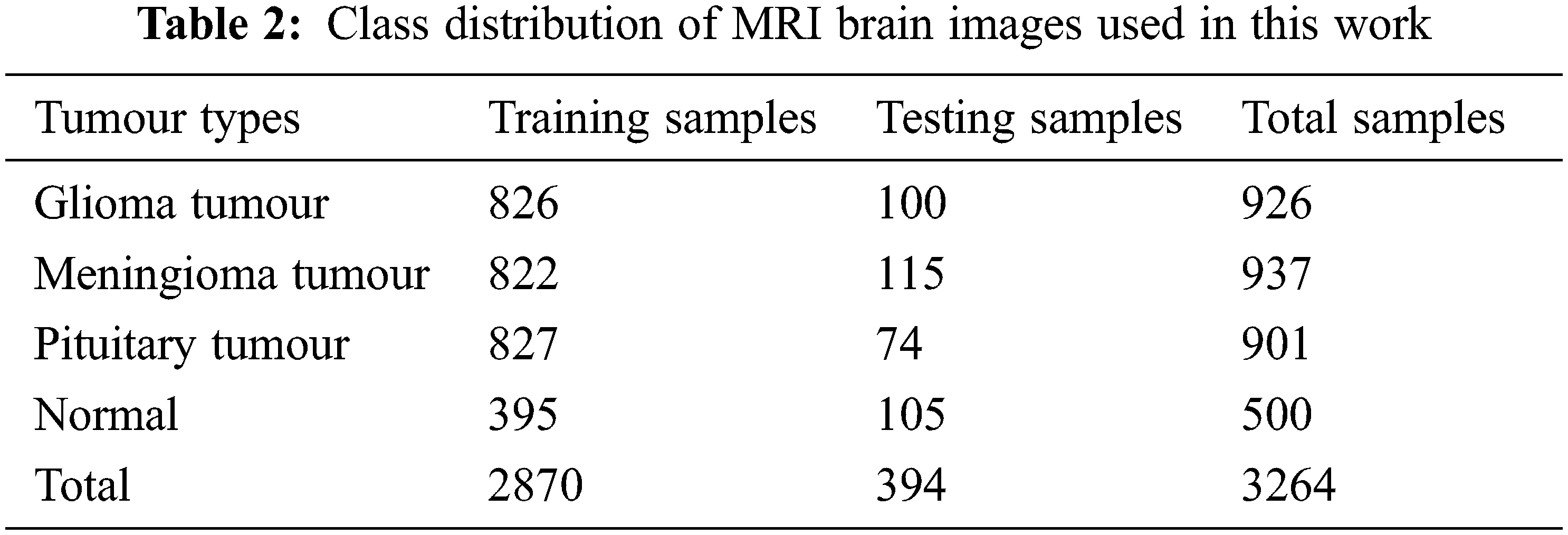
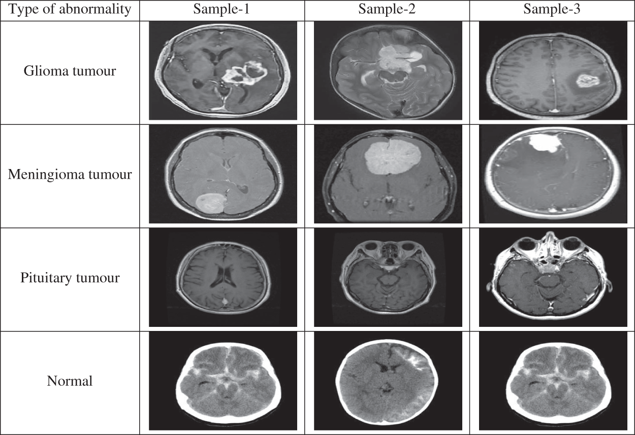
Figure 5: MRI brain images in the database

3.2 Estimation of Metrics

In this study, the performance of the MCC system is estimated by means of performance metrics such as accuracy, sensitivity and specificity. These measures are obtained by forming confusion matrix from the outcomes of the classifiers such as True Positive (TP), False Positive (FP), True Negative (TN) and False Negative (FN). Tab. 3 shows the four-class confusion matrix.

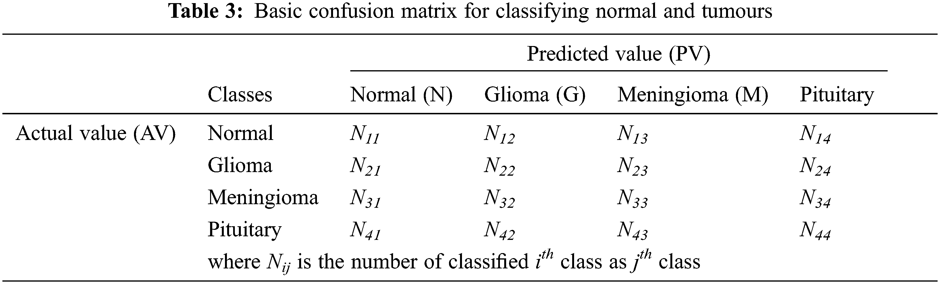
Tab. 4 shows how the parameters such as TP, FP, TN and FN are computed from the confusion matrix in Tab. 3. The third column shows the computed parameters for normal class. Similarly, the performance metrics for other classes can be computed.

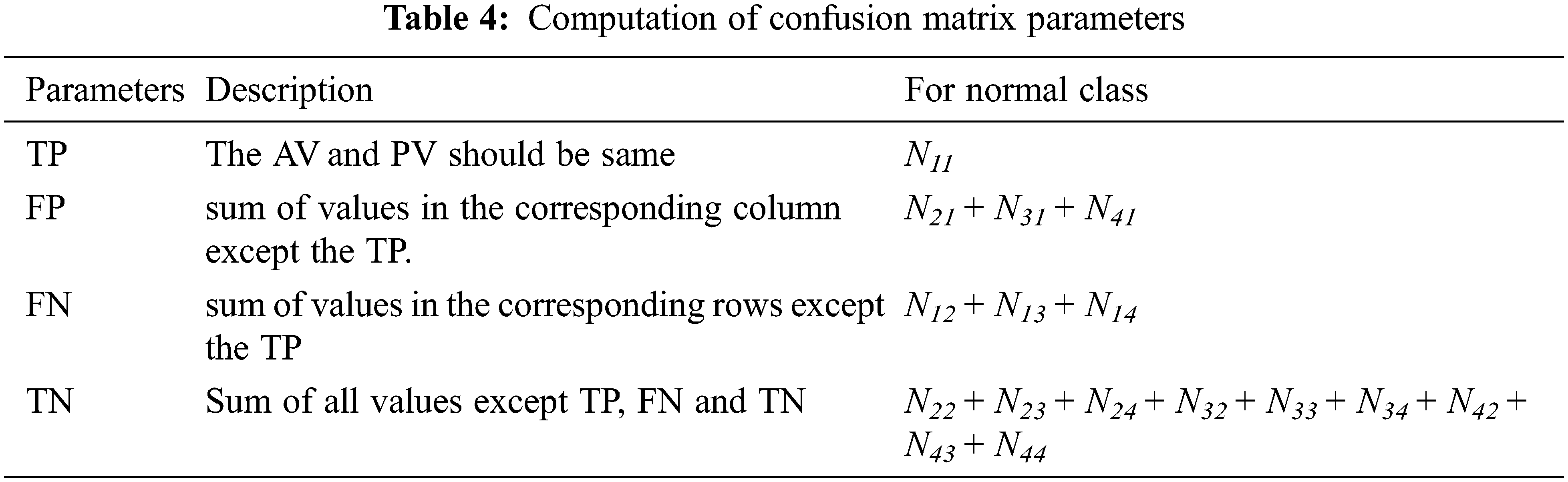
After computing the parameters such as TP, FP, TN and FN, the following Eqs. (23)–(25) are used to obtain the accuracy, sensitivity and specificity of the proposed MCC system for classifying the MRI brain images.

Accuracy=TP+TNTP+FP+TN+FN (23)

Specificity=TNFP+TN (24)

Sensitivity=TPTP+FN (25)

3.3 Performance Analysis

Three machine learning algorithms such as kNN, SVM and RF are employed for classifying MRI brain images into four classes. This section analyzes the individual classifier performances at first and then a comparative analysis is made to show the efficacy of the classifiers.

3.3.1 Performance of MCC System Using kNN

Tab. 5 shows the obtained confusion matrix while using the kNN classifier to classify the features or BRISK and additional image features for MRI brain image classification and Fig. 6 shows the performance measures for each category using Euclidean distance in kNN classifier.

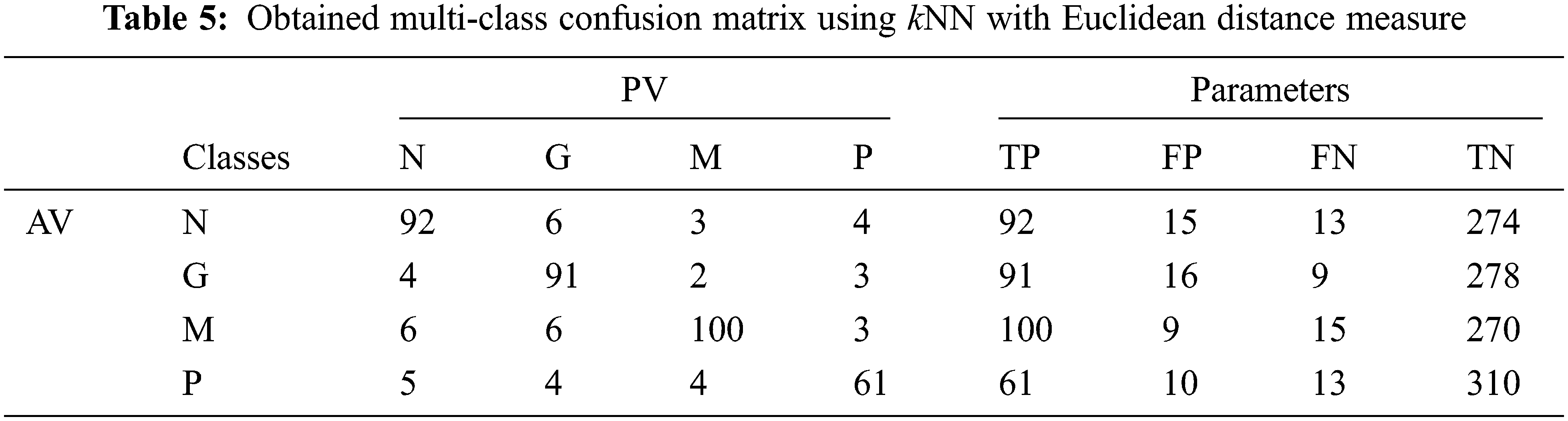
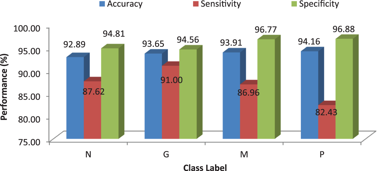
Figure 6: Performances of the proposed MCC system using kNN classifier using Euclidean distance

It can be seen from Fig. 6 that the accuracy of the MCC system using kNN classifier lies between 93% and 94%. Though the system provides significant accurate results, the sensitivity of the system, less than 90% except the glioma pattern (91%). Fig. 7 shows the average performances of kNN classifier using different distance matrices.

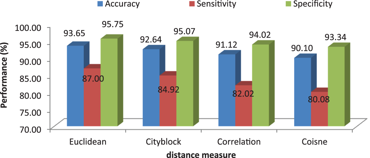
Figure 7: MCC’s system performances using kNN classifier with different distance measures

3.3.2 Performance of MCC System Using SVM

Tab. 6 shows the obtained confusion matrix while using the SVM classifier to classify the features or BRISK and additional image features for MRI brain image classification and Fig. 8 shows the performance measures for each category using SVM classifier with RBF classifier.

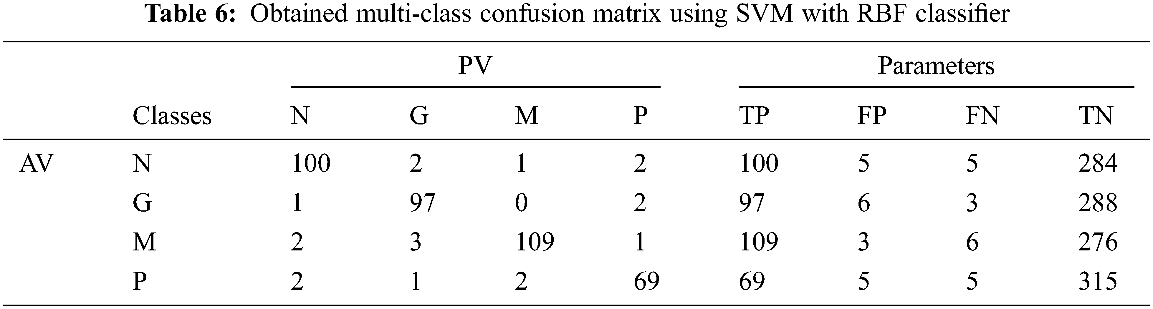
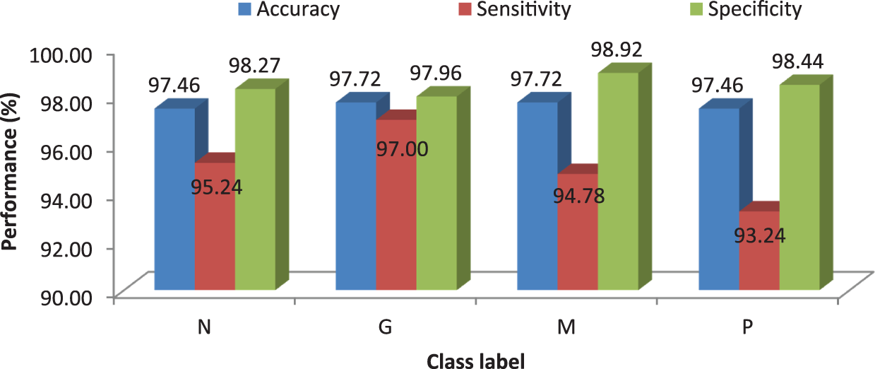
Figure 8: Performances of the proposed MCC system using SVM classifier with RBF kernel

It can be seen from Figs. 6 and 8 that the performance of the proposed MCC system is increased when using SVM classifier than kNN classifier. The accuracy of the MCC system increases minimum by ∼3%. Also, the sensitivity the system is increased from 82.43% (MCC-kNN) to 93.24% by MCC-SVM system. Fig. 9 shows the average performances of SVM classifier using different kernels.

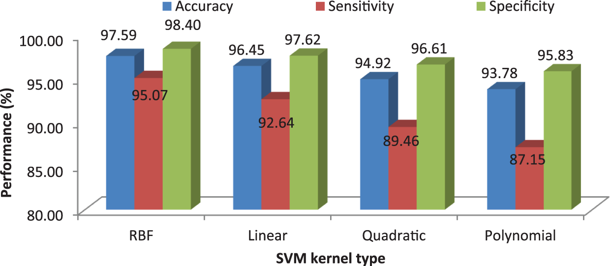
Figure 9: MCC’s system performances using SVM classifier with different kernels

3.3.3 Performance of MCC System Using RF

Tab. 7 shows the obtained confusion matrix while using the RF classifier to classify the features or BRISK and additional image features for MRI brain image classification and Fig. 10 shows the performance measures for each category.

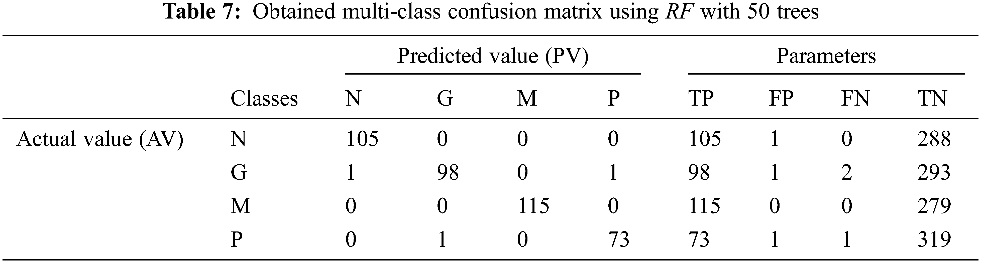
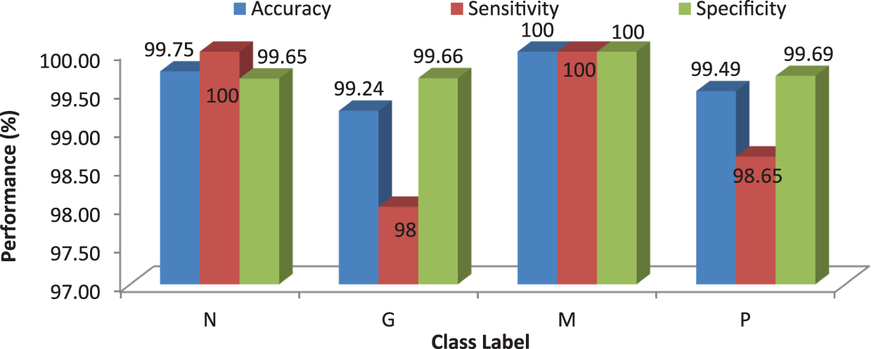
Figure 10: Performances of the proposed MCC system using RF classifier with 50 trees

It can be seen from Fig. 10 that the proposed MCC system provides highest performance while using RF classifier than SVM and kNN. All normal and meningioma MRI brain images are correctly classified and only 2 (glioma) and 1 (pituitary) images are misclassified. This is due to that RF is constructed by a combination of several decision trees and finally takes decision regarding classification. Fig. 11 shows the average performances of RF classifier using different number of trees.

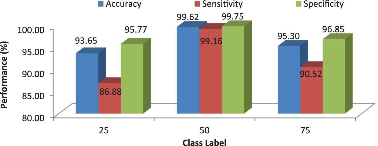
Figure 11: MCC’s system performances using RF classifier for different number of trees

Fig. 12 clearly illustrates the performance analysis of the proposed MCC system for diagnosing brain cancer using different machine learning algorithms.

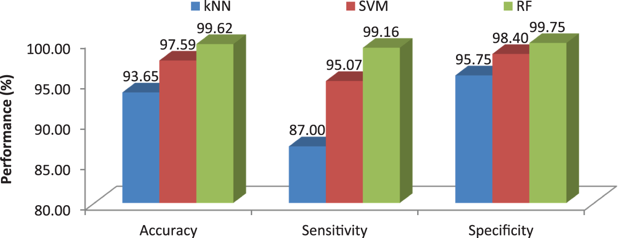
Figure 12: Comparison of machine learning algorithms in terms of average performance metrics

4  Conclusions

This work proposes an efficient BRISK descriptor based MCC system for the diagnosis of brain cancer. It uses MRI images for the classification of three different brain cancers such as glioma, meningioma and pituitary along with normal class. The image based features such as image area, orientation, equivalent, perimeter, diameter, minor and major axis, min, max mean intensity are also extracted and added to BRISK descriptor to increase the MCC system performances. Three machine learning classifiers; kNN, SVM and RF are used for the classification. More than 3000 MRI brain images are employed to access the MCC system’s performances. Results show that the accuracies of MCC system are 93.65% by kNN, 97.59% by SVM and 99.62% by RF classifier. It is observed that the MCC-RF system provides promising results than MCC-kNN and MCC-SVM system.

Funding Statement: The authors received no specific funding for this study.

Conflicts of Interest: The authors declare that they have no conflicts of interest to report regarding the present study.

References

1. L. Hussain, S. Saeed, I. A. Awan, A. Idris, M. S. Nadeem et al., “Detecting brain tumor using machines learning techniques based on different features extracting strategies,” Current Medical Imaging, vol. 15, no. 6, pp. 595–606, 2019. [Google Scholar]
2. J. Kang, Z. Ullah and J. Gwak, “MRI-Based brain tumor classification using ensemble of deep features and machine learning classifiers,” Sensors, vol. 21, no. 6, pp. 1–21, 2021. [Google Scholar]
3. G. R. Kwon, D. Basukala, S. W. Lee, K. H. Lee and M. Kang, “Brain image segmentation using a combination of expectation-maximization algorithm and watershed transform,” International Journal of Imaging Systems and Technology, vol. 26, no. 3, pp. 225–232, 2016. [Google Scholar]
4. D. R. Nayak, R. Dash and B. Majhi, “Brain MR image classification using two-dimensional discrete wavelet transform and AdaBoost with random forests,” Neurocomputing, vol. 177, pp. 188–97, 2016. [Google Scholar]
5. M. Alfonse and A. B. Salem, “An automatic classification of brain tumors through MRI using support vector machine,” Egyptian Computer Science Journal, vol. 40, no. 3, pp. 11–21, 2016. [Google Scholar]
6. A. Kharrat, K. Gasmi, M. B. Messaoud, N. Benamrane and M. Abid, “A hybrid approach for automatic classification of brain MRI using genetic algorithm and support vector machine,” Leonardo Journal of Sciences, vol. 17, no. 1, pp. 71–82, 2010. [Google Scholar]
7. G. Hemanth, M. Janardhan and L. Sujihelen, “Design and implementing brain tumor detection using machine learning approach,” in Int. Conf. on Trends in Electronics and Informatics, Tirunelveli, India, pp. 1289–1294, 2019. [Google Scholar]
8. M. Aarthilakshmi, S. Meenakshi, A. Poorna Pushkala, V. Ramalakshmi and N. B. Prakash, “Brain tumor detection using machine learning,” International Journal of Scientific & Technology Research, vol. 9, no. 4, pp. 1976–1979, 2020. [Google Scholar]
9. K. Sharma, A. Kaur and S. Gujral, “Brain tumor detection based on machine learning algorithms,” International Journal of Computer Applications, vol. 103, no. 1, pp. 7–11, 2014. [Google Scholar]
10. M. N. Wernick, Y. Yang, J. G. Brankov, G. Yourganov and S. C. Strother, “Machine learning in medical imaging,” IEEE Signal Processing Magazine, vol. 27, no. 4, pp. 25–38, 2010. [Google Scholar]
11. G. Manogaran, P. Mohamed shakeel, A. S. Hassanein, P. M. Kumar and G. C. Babu, “Machine learning approach-based gamma distribution for brain tumor detection and data sample imbalance analysis,” IEEE Access, vol. 7, pp. 12–19, 2019. [Google Scholar]
12. Z. Kapás, L. Lefkovits and L. Szilágyi, “Automatic detection and segmentation of brain tumor using random forest approach,” in Int. Conf. on Modelling Decisions for Artificial Intelligence, Sant Julià de Lòria, Andorra, pp. 301–312, 2016. [Google Scholar]
13. M. A. Kabir, “Automatic brain tumor detection and feature extraction from MRI image,” The Scientific World Journal, vol. 8, no. 4, pp. 695–711, 2020. [Google Scholar]
14. M. Al-Ayyoub, G. Husari, O. Darwish and A. Alabed-alaziz, “Machine learning approach for brain tumor detection,” in Proc. of the 3rd Int. Conf. on Information and Communication Systems, Irbid, Jordan, pp. 1–4, 2012. [Google Scholar]
15. H. Byale, G. M. Lingaraju and S. Sivasubramanian, “Automatic segmentation and classification of brain tumor using machine learning techniques,” International Journal of Applied Engineering Research, vol. 13, no. 14, pp. 11686–11692, 2018. [Google Scholar]
16. I. Soesanti, M. H. Avizenna and I. Ardiyanto, “Classification of brain tumor MRI image using random forest algorithm and multilayers perceptron,” Journal of Engineering and Applied Sciences, vol. 15, no. 19, pp. 3385–3390, 2020. [Google Scholar]
17. F. P. Polly, S. K. Shil, M. A. Hossain, A. Ayman and Y. M. Jang, “Detection and classification of HGG and LGG brain tumor using machine learning,” in Int. Conf. on Information Networking, Chiang Mai, Thailand, pp. 813–817, 2018. [Google Scholar]
18. R. Muthaiyan and D. M. Malleswaran, “An automated brain image analysis system for brain cancer using shearlets,” Computer Systems Science and Engineering, vol. 40, no. 1, pp. 299–312, 2022. [Google Scholar]
19. N. Veni and J. Manjula, “Modified visual geometric group architecture for MRI brain image classification,” Computer Systems Science and Engineering, vol. 42, no. 2, pp. 825–835, 2022. [Google Scholar]
20. A. Khalid Alduraibi, “A hybrid deep features PSO-ReliefF based classification of brain tumor,” Intelligent Automation & Soft Computing, vol. 34, no. 2, pp. 1295–1309, 2022. [Google Scholar]
21. S. Leutenegger, M. Chli and R. Y. Siegwart, “BRISK: Binary robust invariant scalable keypoints,” in Int. Conf. on Computer Vision, Barcelona, Spain, pp. 2548–2555, 2011. [Google Scholar]
22. A. Tzotsos and D. Argialas, “Support vector machine classification for object-based image analysis,” in Object-Based Image Analysis, 1st ed., Berlin, Heidelberg: Springer, pp. 663–677, 2008. [Google Scholar]
23. C. Cortes and V. Vapnik, “Support-vector network,” Machine Learning, vol. 20, no. 3, pp. 273–297, 1995. [Google Scholar]
24. Y. B. Bakare and M. Kumarasamy, “Histopathological image analysis for oral cancer classification by support vector machine,” International Journal of Advances in Signal and Image Sciences, vol. 7, no. 2, pp. 1–10, 2021. [Google Scholar]
25. A. Subudhi, M. Dash and S. Sabut, “Automated segmentation and classification of brain stroke using expectation-maximization and random forest classifier,” Biocybernetics and Biomedical Engineering, vol. 40, no. 1, pp. 277–289, 2020. [Google Scholar]
26. Kaggle Repository: https://www.kaggle.com/sartajbhuvaji/brain-tumor-classification-mri. [Google Scholar]
Cite This Article
Copyright © 2023 The Author(s). Published by Tech Science Press.
This work is licensed under a Creative Commons Attribution 4.0 International License , which permits unrestricted use, distribution, and reproduction in any medium, provided the original work is properly cited.
Downloads
Citation Tools