An Intelligent Deep Neural Sentiment Classification Network

1  Introduction

Information extraction from social media has been of interest to researchers in recent years. This section reviews the sentiment analysis systems that have been used to analyze the Twitter data are briefly reviewed in this section. An iterative algorithm is described in [1] for Twitter sentiment analysis. It uses the inter-relationships between the messages. The sentiment diffusion patterns are utilized to improve the sentiment analysis. The interesting properties are identified by the sentiment reversal phenomenon. An extended sentiment dictionary-based analysis of Chinese text is discussed in [2]. The dictionary consists of basic words, sentiment words, and polysemic sentiment words. It uses Naive Bayes (NB) classifier, and by utilizing the sentiment score rules, the sentiment is classified.

Fuzzy-based sentiment analysis is discussed in [3] for Twitter data. It models the syntactic information of words with their sentiment context. It uses the feature ensemble method to analyze the tweets with fuzzy sentiments by considering the lexical, position, and word type with the sentiment polarity of words. A semantic conceptualization is discussed in [4] for sentiment analysis using tagged bag-of-concepts. The relations and vital information between the messages are preserved while analyzing the text to uncover latent sentiments.

A hybrid neural network model is discussed in [5] to analyze public emotion. The latent semantic relationships with co-occurrence statistical features between words are used for the analysis. Several filters are used in the multi-channel Convolution Neural Network (CNN) with varying window sizes to represent the sequence of words. Also, the sentence representations are obtained via Long Short Term Memory (LSTM) network. Feature-based sentiment analysis system is discussed in [6] for Twitter data with improved negation. It uses lexicon-based features, n-gram features, and morphological features. NB, decision tree, and Support Vector Machine (SVM) classifiers are used for classification.

A multi-task ensemble approach is discussed in [7] for predicting sentiment, emotion, and intensity. It uses CNN, LSTM, and gated recurrent unit models for the prediction with the help of hand-craft features. Deep belief network based sentiment analysis is discussed in [8]. It analyzes the data using deep learning to create the feature vector. Then, noise reduction is employed to improve the system’s accuracy. A spectral clustering based approach is discussed in [9] for lexicon construction in social networks. At first, a filtering text mode is used to compute the text influence value. Then, a sentiment relationship model is constructed using the similarities from base, topic, and synonym sentiment. Finally, a clustering model is employed for the analysis.

A combination of two clustering approaches is discussed in [10] for sentiment analysis using Twitter data. It combines the k-means and density based clustering to categorize the tweets into positive, neutral, and negative. A binary clustering framework is described in [11] for Twitter sentiment analysis. A co-operative system of three clustering approaches of linkage technique; single, complete, and average is designed for optimal cluster selection. SVM and NB classifiers are employed for the classification. Two LSTM directions are used for effective sentiment analysis in [12]. The CNN and bi-directional LSTM are integrated to extract local features after applying the word embedding model. The smaller dimension of features from the CNN model is used to LSTM for the analysis.

An ordinal regression based sentiment analysis is discussed in [13]. It extracts features such as term frequency-inverse document frequency after removing the unwanted characters in the tweets such as hyperlinks, re-tweets, and user names. These features are then classified using SVM, random forest, NB, and logistic regression. Deep CNNs are employed in [14] for Twitter sentiment analysis. The latent semantic relationships with co-occurrence statistical features between words are used to design the word embedding method. It is combined with n-grams to form a feature vector. Also, the word sentiment polarity score features are used.

The main goal of this work is the development of a Deep Neural Sentiment Classification Network (DNSCN) that can be used to analyze Twitter tweets and classify them. The deep learning techniques will be more efficient and appropriate for extracting information. This work develops a deep network named DNSCN for Twitter tweets classification. The rest of the paper is organized as follows: Section 2 discusses the DNSCN that implements the algorithm for Twitter data. The algorithm’s effectiveness is evaluated in Section 3 using Twitter datasets; TSA2, TSA3, and TDS. Section 4 concluded the work by summing up the work done so far.

2  Methods and Materials

The information extraction systems are built for different tasks such as movie reviews, financial news, and product reviews. These tasks often differ from each other. Fig. 1 shows the four primary modules of information extraction systems.

Figure 1: Core elements in information extraction systems

In addition to the modules in Fig. 1, extra modules are required for a particular application based on the requirements. Tokenization is the process of segmenting text documents into word translation. The input sequence is processed in the lexical analysis module and converted into tokens (sequence of symbols). The grammatical structure is determined by parsing the tokens in the syntactic analysis module with respect to a given grammar. The proposed DNSCN architecture for the classification of Twitter data consists of the following modules; Data Preparation (DP), Data Representation (DR), Analysis Model (AM), and Testing.

2.1 DP Module

In the DP module, the given text data is cleaned first as it is impossible to fit the raw data by the deep learning model. Fig. 2 shows how the data cleaning is done in the proposed system. After loading the data, the first step is to split the raw data into text sentences, split the words into tokens based on white space, and then make them all lower case words. Finally, the stop words, numerical data, and punctuations are removed to get the clean data.

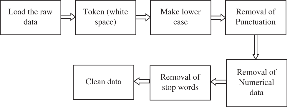
Figure 2: Process to clean up the data in the DP module

2.2 DR Module

In the DR module, two models; Bag-of-Words (BoW) and Word Embeddings (WE) are employed to represent the cleaned data from the DP module. The BoW model has shown great success in document classification and language modeling problems [15]. The main problem of deep learning networks is that they can’t work with the raw text data. The raw text data must be converted into vectors of numbers. This process is named feature encoding or information extraction.

The collected tweets are represented by their BoW. It discards the order of words in the Twitter tweets. In machine learning, it is also called attribute-value representation. The token in the cleaned data from the DP module are characterized as attributes. The values are obtained from the corresponding weights of the tokens. A weight is assigned based on the words in each tweet. It is noted that more dominant features have more weight. Fig. 3 shows the process of BoW representations.

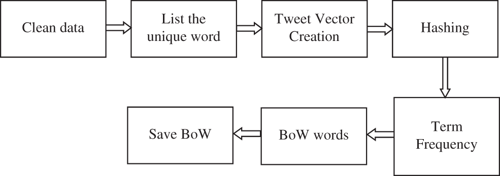
Figure 3: Process of BoW representation

Reducing the vocabulary size for predictive models of text data is important. If the vocabulary list is larger, then the representation of these tweets is sparser. To overcome this, unique words are selected. The next step is the Tweet Vector Creation (TVC) which makes the tweets into a vector so that the proposed DNSCN architecture can use them as inputs. In TVC, a fixed-length tweet representation is used. As the data is cleaned in the DP module, each tweet may contain a few vocabularies in the TVC. The high-frequency words are dominated in the TVC when scoring word frequency. To avoid this, the frequency of words is rescaled by their appearance in all tweets, which is referred to as term frequency.

Another representation, the WE model is also used for the representation that provides similar representation for similar words. Each unique word in the tweets is represented in the embedding space by a point. These points are learned in such a way that they learn something about the meaning of the tweets. This work uses the Word2Vec scheme developed by Google. In order to simplify the WE module’s learning process, the pretrained Word2Vec model is used [16].

2.3 AM Module

In this module, the proposed DNSCN architecture is implemented to classify tweets. The arrangement of layers is shown in Fig. 4 for extracting deep features.

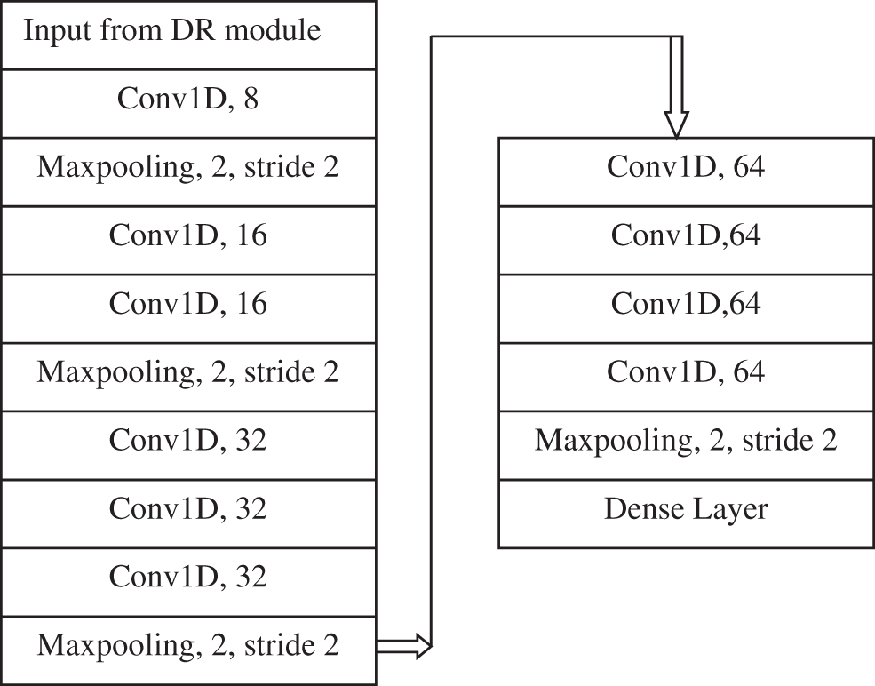
Figure 4: Deep feature extraction

This module uses one-dimensional convolution filters (1 × 3), and a max-pooling layer (1 × 2) with the stride of 2 is employed. The number of shifts over the vectors is termed as stride. For a stride of 2, the convolution filter is moved to two values in the input vector. It can be seen from Fig. 4 that the number of convolution filters used in this work increase from 8 to 64 in multiples of power two, and the number of convolution layer increases from 1 to 4 while increasing the filter size. The convolution operation for an input vector (x) with weights (w) by the convolution filter is defined in Eq. (1).

yj=∑i=−ppxj−iwi (1)

The final max-pooling layer produces the reduced deep features for the next step. Table 1 shows how the max-pooling layer works.

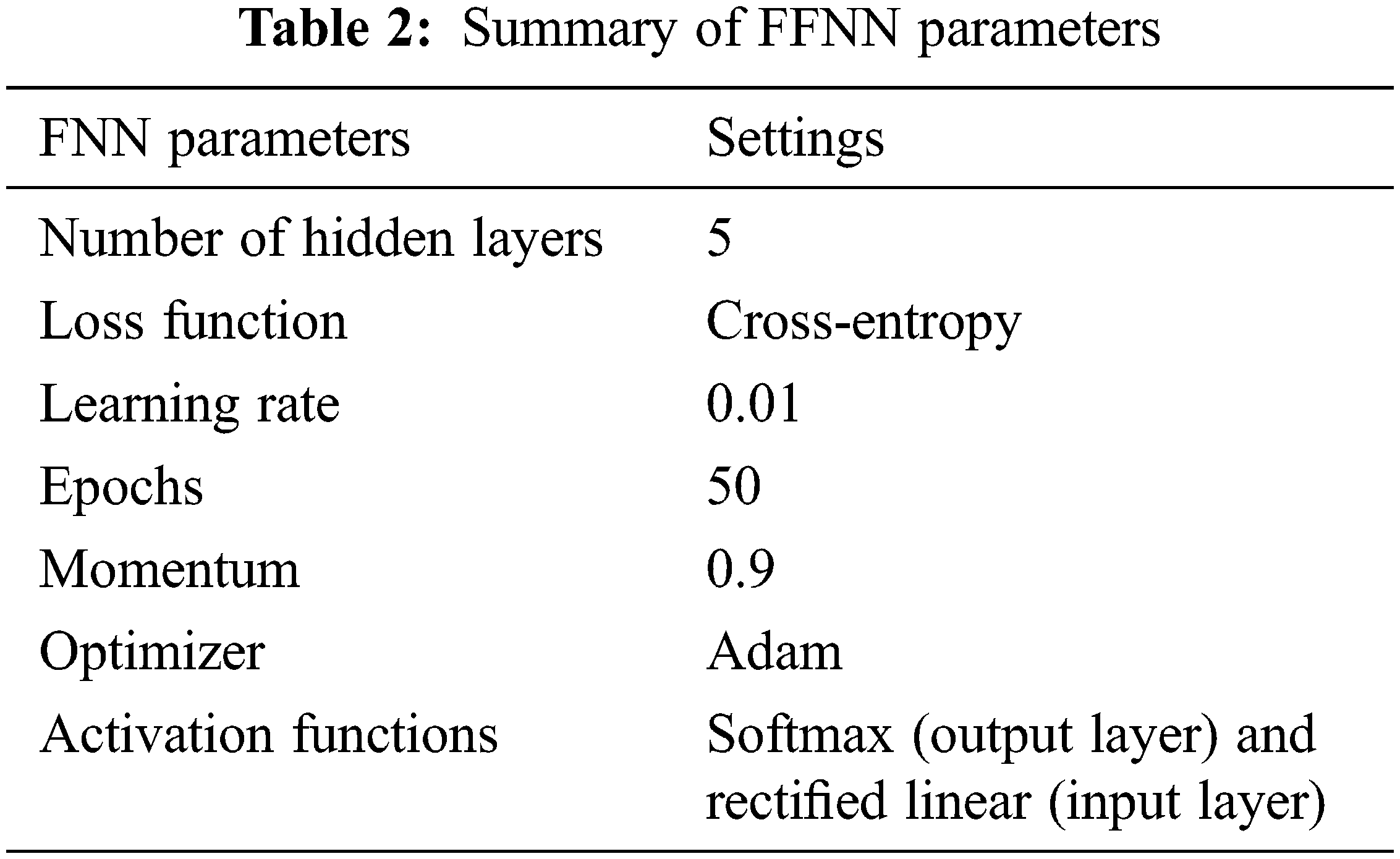
The classification is achieved in the dense layer where Feed Forward Neural Network (FFNN) is used. In the FFNN, the cross-entropy loss is employed during training, and Adam optimizer with 50 epochs. The cross-entropy loss ( CEL ) is defined in Eq. (2).

CEL=−∑j=1ctclog⁡(pc) (2)

where the probability for the ith class is pi and its truth label is ti . During training, the developed model weights are adjusted so that the CEL should be minimized. The learning rate controls the weight adjustment based on the loss gradient. The backpropagation algorithm is commonly used for training the FFNNs. It consists of the forward and the backward pass. The FFNN is initialized by setting random weights with rectified linear activation function. In the forward pass results from the computation at each neuron from each layer pass through the network layer by layer resulting in the actual output. There is no adaptation of weights in the forward pass. The actual output is subtracted from the desired output in the backward pass. If there is no error, weights are not changed; otherwise, the error is propagated from the output in the direction of the inputs and at each layer computing the local gradient for each neuron and simultaneously adjusting weights.

The training set is repeatedly presented to the network until the Euclidean norm of the gradient reaches a certain threshold or when the mean square error attains a constant value. The weights are then saved (frozen). These weights contain information about the underlying structure between inputs and the corresponding targets. The classifier uses this knowledge (saved weights) on test data (data that has not been seen before). The test data is presented using just the feed-forward calculations. Table 2 shows the summary of the FFNN parameters used in this study.

3  Results and Discussions

To evaluate the effectiveness of the proposed DNSCN system, experiments are carried out on three Twitter datasets; Twitter-sanders-apple [17] and Twitter dataset [18]. The former dataset has two subsets, TSA2 (2-classes) and TSA3 (3-classes). Based on the information in the tweets, they are classified into positive, negative, and neutral tweets. Table 3 shows sample tweets in each category, and the distribution of tweets in these databases is shown in Fig. 5.

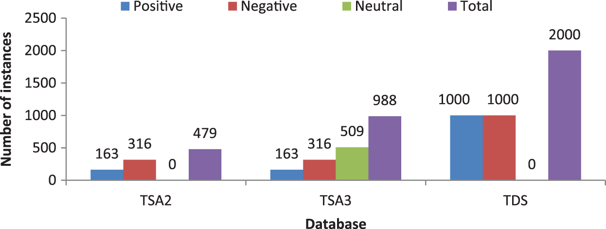
Figure 5: Distribution of tweets in the databases used in this work

As the number of classes varies in each database, the proposed SAS system performs binary (TSA2 and TDS) and multi-class classification (TSA3) on tweeter databases. The performance of DNSCN architecture on Twitter databases can be evaluated by precision and recall metrics. These metrics are defined using three terms; True Positive (TP), False Positive (FP), and False Negative (FN). TP represents the number of correctly classified samples for a particular class a. For the same class, FP represents the number of other classes misclassified to class a, and FN represents the number of samples from class a misclassified. Precision is defined in Eq. (3) and Recall is defined in Eq. (4).

Precision=#TP#TP+#FP (3)

Recall=#TP#TP+#FN (4)

Based on these performance metrics, the relative performance (F1 score) of the proposed DNSAS architecture can be evaluated by combing both. F1 score is defined in Eq. (5).

F1score=2×Precision×RecallPrecision+Recall (5)

The cross-validations are applied to validate the proposed DNSCN architecture. It uses two cross-validation protocols 5-fold and 10-fold for the evaluation. A sample 5-fold validation approach is shown in Fig. 6.

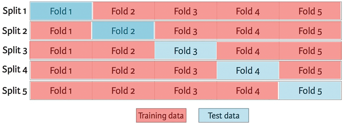
Figure 6: 5-fold cross validation protocols

It can be seen from Fig. 6 that for 5-fold cross-validation, the whole database is divided into five folds with an equal number of samples from each class, and the performance of the proposed system is analyzed five times. At each iteration or split, only one fold is used for testing, and the remaining is used for training the classifier. At last, all the outputs are averaged to get the final result.

Along with the validation protocols, the proposed system is tested for the representation models; BoW and WE. The binary classification performances of the proposed DNSCN architecture on TSA2 and TDS databases are discussed at first. Figs. 7 and 8 show the performances of the DNSCN-BoW model, and the DNSCN-WE model on the TSA2 database for 5-fold and 10-fold respectively.

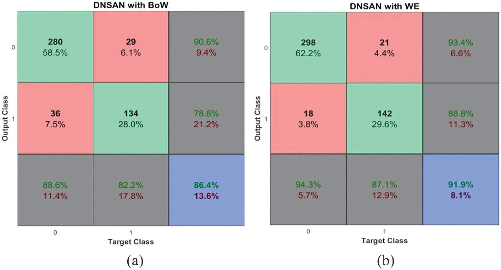
Figure 7: Performances on TSA2 database (a) DNSCN-BoW (5-fold) (b) DNSCN-WE (5-fold)

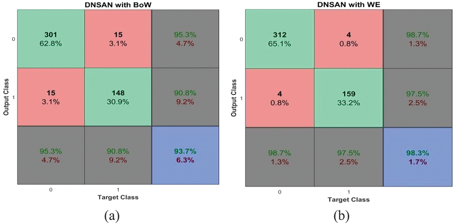
Figure 8: Performances on the TSA2 database (a) DNSCN-BoW (10-fold) (b) DNSCN-WE (10-fold)

Fig. 9 shows the performances of the DNSCN-BoW model and the DNSCN-WE model on the TDS database for 5-fold and 10-fold respectively.

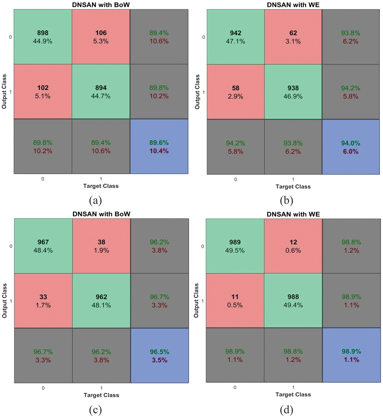
Figure 9: Performances on the TDS database (a) DNSCN-BoW (5-fold) (b) DNSCN-WE (5-fold) (c) DNSCN-BoW (10-fold) (d) DNSCN-WE (10-fold)

The multi-class classification performances of the proposed DNSCN architecture on the TSA3 database are discussed. Fig. 10 shows the performances of the DNSCN-BoW model and the DNSCN-WE model on the TSA3 database for 5-fold and 10-fold respectively.

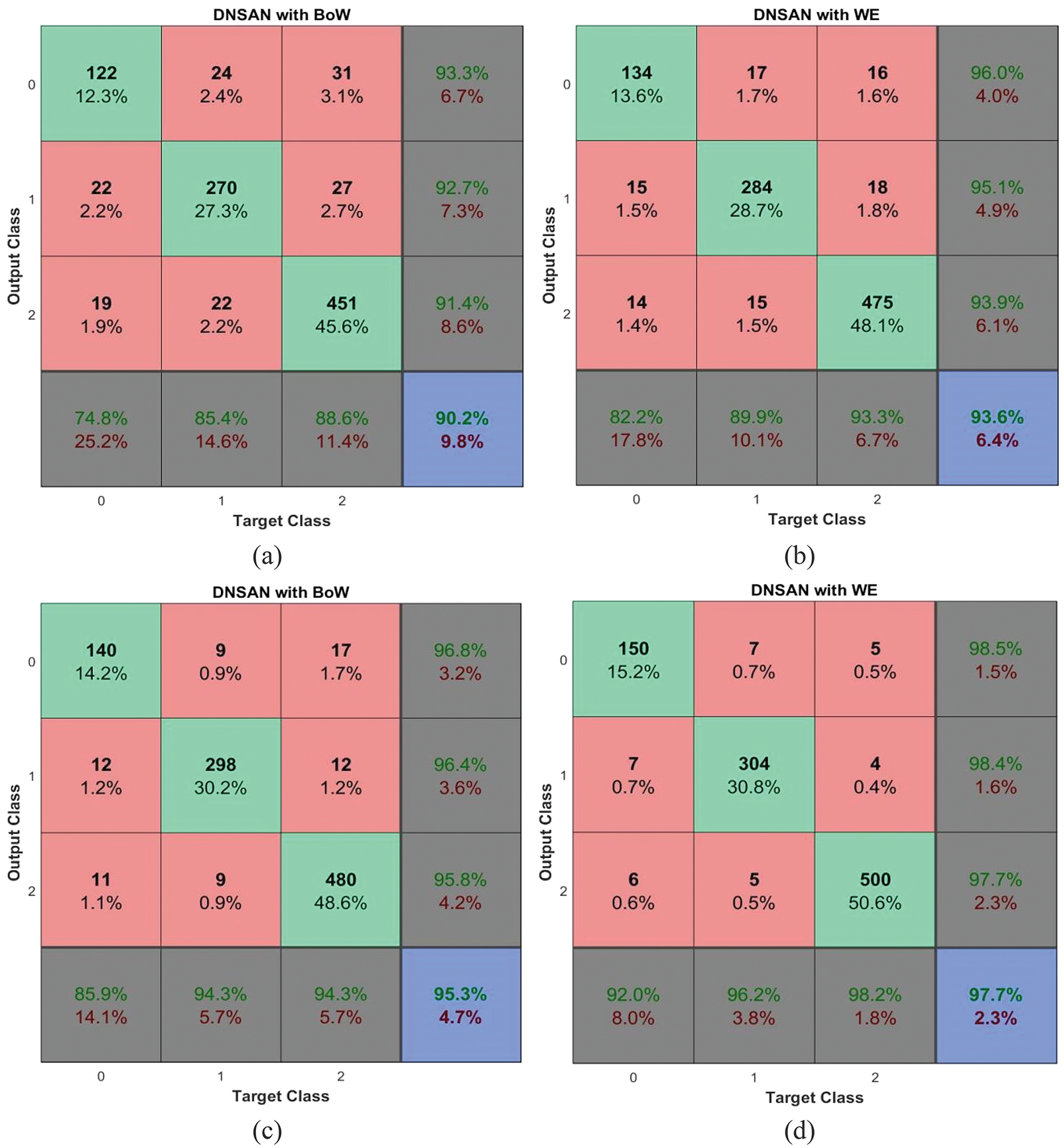
Figure 10: Performances on the TSA3 database (a) DNSCN-BoW (5-fold) (b) DNSCN-WE (5-fold) (c) DNSCN-BoW (10-fold) (d) DNSCN-WE (10-fold)

Table 4 summarizes the performances of the proposed DNSCN architecture for Twitter data classification from the performances shown in the above figures.

It can be seen from the summary Table 4 that the performance of the proposed DNSCN architecture provides better results for the 10-fold validation protocol than for the 5-fold validation protocol for all datasets. This is due to the network train from the more number of samples in the 10-fold validation protocol. Also, it is noted that the WE model provides more accuracy than the BoW model for representing the tweets in the feature encoding.

4  Conclusions

This study developed a deep learning framework for analyzing Twitter data. It focuses on a BoW and WE model to extract the features from the cleaned data. To clean the data, a small pipeline of preprocessing techniques; split the raw data into text sentences, split the words into tokens, make lower case words, remove the stop words, numerical data, and punctuations are employed. After representation, the proposed DNSCN architecture is used to classify tweets into different classes. Three validation protocols, 2-fold, 5-fold, and 10-fold are employed. Results show that the proposed DNSCN architecture can extract the statistically significant features from the Twitter corpus and automatically classify them. Also, it can able to extract domain-specific information. The implementation of DNSCN architecture has been demonstrated on three Twitter databases, TSA2, TSA3, and TDS, in terms of F1 score, precision, and recall.

Funding Statement: The authors received no specific funding for this study.

Conflicts of Interest: The authors declare that they have no conflicts of interest to report regarding the present study.

References

 1.  L. Wang, J. Niu and S. Yu, “SentiDiff: Combining textual information and sentiment diffusion patterns for twitter sentiment analysis,” IEEE Transactions on Knowledge and Data Engineering, vol. 32, no. 10, pp. 2026–2039, 2020. [Google Scholar]

 2.  G. Xu, Z. Yu, H. Yao, F. Li, Y. Meng et al., “Chinese text sentiment analysis based on extended sentiment dictionary,” IEEE Access, vol. 7, pp. 43749–43762, 2019. [Google Scholar]

 3.  H. T. Phan, V. C. Tran, N. T. Nguyen and D. Hwang, “Improving the performance of sentiment analysis of tweets containing fuzzy sentiment using the feature ensemble model,” IEEE Access, vol. 8, pp. 14630–14641, 2020. [Google Scholar]

 4.  Y. S. Mehanna and M. B. Mahmuddin, “A semantic conceptualization using tagged bag-of-concepts for sentiment analysis,” IEEE Access, vol. 9, pp. 118736–118756, 2021. [Google Scholar]

 5.  M. Ling, Q. Chen, Q. Sun and Y. Jia, “Hybrid neural network for sina weibo sentiment analysis,” IEEE Transactions on Computational Social Systems, vol. 7, no. 4, pp. 983–990, 2020. [Google Scholar]

 6.  I. Gupta and N. Joshi, “Feature-based twitter sentiment analysis with improved negation handling,” IEEE Transactions on Computational Social Systems, vol. 8, no. 4, pp. 917–927, 2021. [Google Scholar]

 7.  M. S. Akhtar, D. Ghosal, A. Ekbal, P. Bhattacharyya and S. Kurohashi, “All-in-one: Emotion, sentiment and intensity prediction using a multi-task ensemble framework,” IEEE Transactions on Affective Computing, vol. 13, no. 1, pp. 285–297, 2022. [Google Scholar]

 8.  R. Chen and Hendry, “User rating classification via deep belief network learning and sentiment analysis,” IEEE Transactions on Computational Social Systems, vol. 6, no. 3, pp. 535–546, 2019. [Google Scholar]

 9.  B. Zhang, D. Xu, H. Zhang and M. Li, “STCS lexicon: Spectral-clustering-based topic-specific Chinese sentiment lexicon construction for social networks,” IEEE Transactions on Computational Social Systems, vol. 6, no. 6, pp. 1180–1189, 2019. [Google Scholar]

10. H. Rehioui and A. Idrissi, “New clustering algorithms for twitter sentiment analysis,” IEEE Systems Journal, vol. 14, no. 1, pp. 530–537, 2020. [Google Scholar]

11. M. Bibi, W. Aziz, M. Almaraashi, I. H. Khan, M. S. A. Nadeem et al., “A cooperative binary-clustering framework based on majority voting for twitter sentiment analysis,” IEEE Access, vol. 8, pp. 68580–68592, 2020. [Google Scholar]

12. S. Tam, R. B. Said and Ö. Ö. Tanriöver, “A convBiLSTM deep learning model-based approach for twitter sentiment classification,” IEEE Access, vol. 9, pp. 41283–41293, 2021. [Google Scholar]

13. S. E. Saad and J. Yang, “Twitter sentiment analysis based on ordinal regression,” IEEE Access, vol. 7, pp. 163677–163685, 2019. [Google Scholar]

14. Z. Jianqiang, G. Xiaolin and Z. Xuejun, “Deep convolution neural networks for twitter sentiment analysis,” IEEE Access, vol. 6, pp. 23253–23260, 2018. [Google Scholar]

15. D. Yan, K. Li, S. Gu and L. Yang, “Network-based bag-of-words model for text classification,” IEEE Access, vol. 8, pp. 82641–82652, 2020. [Google Scholar]

16. S. Ji, N. Satish, S. Li and P. K. Dubey, “Parallelizing word2vec in shared and distributed memory,” IEEE Transactions on Parallel and Distributed Systems, vol. 30, no. 9, pp. 2090–2100, 2019. [Google Scholar]

17. Twitter-sanders-apple database: http://boston.lti.cs.cmu.edu/classes/95-865-K/HW/HW3/. [Google Scholar]

18. Twitter dataset: https://drive.google.com/file/d/0BwPSGZHAP_yoN2pZcVl1Qmp1OEU/view?resourcekey=0-G-0AzTVFV_4wgJoxhgsKFQ. [Google Scholar]