Automatic Detection and Classification of Insects Using Hybrid FF-GWO-CNN Algorithm

1  Introduction

Agriculture is the backbone of the Indian economy since 75 per cent of the population depends on it directly and indirectly. Increased agricultural demand is significant in developing a plant and enhancing its production [1]. Environmental concerns like usage of pesticides, ecological degradation of natural resources, expansion of global trade, growth of human population, changes in consumer patterns and technological advancements have resulted in a new agricultural revolution. This revolution uses digital tools to boost productivity and enhance agricultural input management [2]. Improved agricultural tools allow farmers to examine the spatial-temporal variability of several crucial parameters influencing plant health and yield. These data are collected by sensors to aid decision-making. Since agricultural insects are regarded as crucial elements in a global agricultural economy, regulating those elements using programs like insect population management and dynamic surveys via monitoring systems is essential. The existence of numerous pest species in crops is a significant hazard in the field of agriculture. The manual classification s takes a long time and is not accurate enough in the pest detection process [3].

Computer-based approaches can improve proper plant protection procedures and agriculture operations. Since the traditional manual pest classification methods consume much time and require lots of labour, computer-based approaches have become more prevalent in efficiently classifying pests. However, development in agricultural pest identification has declined dramatically in recent years, and new computer vision systems with machine learning as fully prepared formulas cannot reach satisfactory pest detection capability [4]. Image processing-based approaches are employed for detecting and classifying crop pests in this context. Reports reveal that incorporating deep learning models in image processing has been explored recently and generates enhanced results [5–9]. In the utilization of image processing algorithms, four processes like removing the background by pre-processing, segmenting the contaminated section, extracting the distinguishing features for further analysis and classifying the features using unsupervised clustering or supervised classification algorithms are involved [10–13].

The salt and pepper noise that denotes black and white pixels in the deteriorated image is one of the noises which affects image quality in a broader range. Smoothing filters are frequently applied to the images to reduce the noise variance. A balance has to be maintained between the goal of reducing noise variance and the demand for preserving important image information [14]. Filters that are generally adopted for denoising images and preserving the edge information are bilateral filter [15], total variation filter [16], median filter [17], guided filter [18], and non-local mean filter [19] and anisotropic diffusion filter [20]. These filters require several iterations for the detection of noisy pixels, and these filters show poor stability. Hence, this study has opted for an adaptive median filter, effectively reducing the misclassified number of pixels. The pre-processed image is then divided into homogeneous regions, and the corresponding contours are located accurately [21]. The fuzzy C-means clustering [22] is a widely used approach for segmentation, but it fails to rectify the issues like noise, partial volume effects and non-uniformness of intensity. Modifications in these conventional methods reduce the segmentation accuracy, and these approaches have not considered the frequency bias field of the image. Watershed segmentation is another widely utilized approach, which generates a complete division of images into separate regions [23]. However, it leads to over-segmentation, which divides the images into numerous regions. Hence, an unsupervised method named expectation-maximization algorithm (EMA) is exploited in this study, which estimates the density of data points performing assignments of soft clusters. Then, the feature descriptors are extracted from images, in which the reliable matching points between the noisy and original images are found. Scale Invariant Feature Transformation (SIFT) [24] is a robust method for detecting distinct invariant features of an image, but it is less effective. C-SIFT is another widely used algorithm for extracting local invariant features of a colour image, but its direct application toward multispectral images with more bands is impossible. Hence, the Genomic Algebra SIFT (GA-SIFT) is used, which is powerful but shows increased computational burden. Considering these shortcomings, the Speeded Up Robust Feature (SURF) is employed in this work. It performs an effective and robust description of features with precise image details. Finally, the classification of images has to be performed with improved accuracy. Various machine learning approaches are utilized in this process, but classification accuracy relies on the extracted feature design, increasing computational complexity. Therefore, deep learning is applied to classify larger data sets and solve more complicated issues. Deep learning approaches based on Convolutional Neural Networks (CNN) [25–28] are widely utilized for efficient classification with increased accuracy and convergence speed. This classification approach is optimized by various statistical algorithms, among which Firefly (FF) [29] and Grey Wolf Optimization (GWO) [30] are utilized in this approach. The hybridization of GWO and FF enhances the CNN classifier’s performance, resulting in improved accuracy and a high convergence rate.

This paper proposes an efficient image processing approach for pest detection in crops. Initially, denoising and pre-processing of an input image are performed by an adaptive median filter. The filtered image is segmented by the EMA approach, in which clustering is carried out to estimate data point density. After completing the segmentation process, the desired best features are extracted by the SURF technique. Finally, the images are classified with an improved convergence rate by the hybrid FF-GWO-CNN algorithm. The remaining part of this work includes the description of the proposed image processing-based approach for pest detection in Section 2, the validation of obtained simulation results with comparison plots in Section 3 and the summation in Section 4.

2  Proposed Approach for Pest Detection

The rapid advancement of digital technology has made image processing approaches employed in agricultural research to assist researchers in solving complex problems. The analysis of the image offers a realistic chance for the automation of pest detection in crops. Automated pest identification is highly beneficial for producers with extensive agricultural lands and limited pest scouting skills. This paper proposes an efficient image processing-based approach utilizing a hybrid FF-GWO-CNN algorithm to detect crop pests. The process flow of the proposed methodology is shown in Fig. 1.

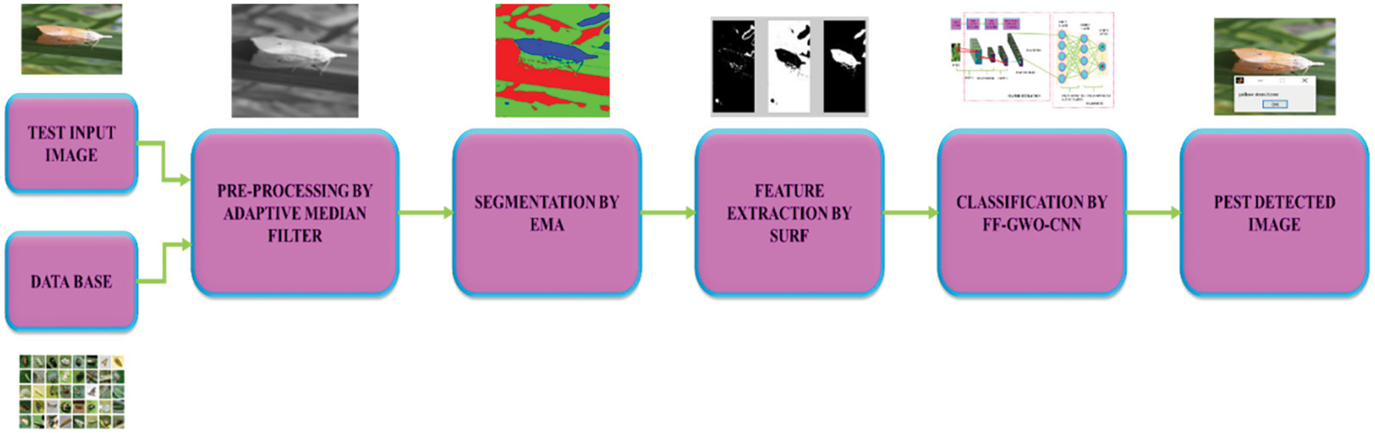
Figure 1: Proposed process flow

An input crop image is initially exposed to pre-processing by an adaptive median filter, which performs denoising and reduces misclassified pixels. The filtered image is further segmented into multiple regions by an iterative process known as EMA, which is insensitive to rotation, scaling and absence of contrast. After the segmentation, the SURF approach describes features that retain the image details. Classification is the final process in which the hybrid FF-GWO-CNN algorithm performs effective pest detection with improved accuracy.

2.1 Pre-Processing by Adaptive Median Filter

The adaptive median filter employs noise detection and filtering algorithms to remove the impulsive noise. The window size utilized for image pixel filtering has adaptive characteristics. If a particular condition is not met, the window size is increased, whereas the median value of the window is utilized for filtering the pixel when the condition is met. Consider Pij as the corrupted image pixel, Pmin as the minimum pixel value, Pmax as the maximum pixel value, S as the current window size, Smax as the maximum window size attained and Pmed as the assigned median of the window, the algorithm for filtering using an adaptive median filter requires two stages, described as follows.

Stage 1:

i)   If Pmin<Pmed<Pmax The median value is not an impulse; hence, the algorithm moves to stage 2 whether the present pixel is an impulse.

ii)   Otherwise, the window size is increased, and stage 1 is repeated till the value of median does not equal an impulse enabling the algorithm to move to stage 2; else, the window size of the maximum value is attained in which the value of median is assigned to the filtered value of image pixel.

Stage 2:

i)   If Pmin<Pmed<Pmax The present value of a pixel is not an impulse; hence, the image pixel filtered remains unchanged.

ii)   Otherwise, the pixel value of the image is equal to either Pmax or Pmin and hence, the image pixel filtered is assigned to the median value from stage 1.

Initially, the size of the filtering window of each noise pixel is selected as 3×3. When the count of uncorrupted window pixels equals at least three, the median of the uncorrupted pixels substitutes the corrupted pixel. Otherwise, the window sides extend iteratively outward by one pixel until the uncorrupted pixel count equals at least three. Subsequently, all pixel medians replace the noise pixel in the filtering window in the following iterations; hence, the image’s filtering is adaptive.

2.2 Segmentation by Expectation-Maximization Algorithm

The EM algorithm is utilized to determine the maximum probability and is widely adopted for estimating data point density through unsupervised segmentation. It performs the stages of expectation (E) and maximization (M) iteratively till the convergence of results. The likelihood expectation is determined in E-stage with the inclusion of latent variables. In the M-stage, the maximum likelihood of parameters is carried out depending on the final E-stage with the maximization of expected likelihood. Another E-stage gets initiated depending on the parameters obtained in the M-stage, and the process gets repeated until the convergence is satisfied. The proposed algorithm divides the image into clusters, and the data points are assigned partially to various clusters replacing the assignment to a single cluster. A probabilistic distribution of partial assignment models in every cluster. The cluster’s centre is updated with relevance to the assigned data points, and the approach gets repeated till the labels of a cluster are not varied considering each cluster. The EMA demands the model parameter initialization of a Gaussian mixture. Assume that there exists a finite count of grey-scale probability density function F . A single Gaussian function is used for modelling every pixel distribution. The shape of the probability density is given by,

P(y|ψ)=∑j=1F⁡πjP(y|μj,∑j) (1)

Here, y represents the characteristic vector, ∑j=1Fπj=1,πj≥0 . The parameter ψ comprises co-variance ∑j, mean μj, mixing coefficients πj for j=1,2,….F. Therefore,

P(y|μj,∑j)=1(2π)d/2|∑|1/2e−1(y−μj)t∑j−1⁡(y−μj)2 (2)

The steps followed by EMA are mentioned below.

Step 1: Initialize co-variance ∑j , mixing coefficient πj and mean μj and further, compute the initial value of log-likelihood, which is expressed as,

logl(ψ)=∑i=1N⁡log[∑j=1F⁡πjP(y|μj∑j)] (3)

Step 2: E-stage

Evaluate the expectancy utilizing the present value of parameters.

Eij=πjP(yi|μj∑j)∑m=1F⁡πmP(yi|μm∑m),1≤j≤F≤i≤N (4)

Step 3: M-stage

The updated mean is obtained as,

μjup=1Nj∑i=1N⁡Eijyi,1≤j≤F (5)

The updated co-variance is given by,

μjup=1Nj∑i=1N⁡Eij(yi−μjup)(yi−μjup)t,1≤j≤F (6)

The updated mixing coefficient is given by,

πjup=NjN1≤j≤F (7)

In which, Nj=∑i=1N⁡Eij .

The algorithm returns to E-stage when the convergence criterion is not satisfied. The segmented image is further subjected to feature description, which is explained in the next section.

2.3 Feature Description by SURF Approach

The selection of the best possible features of the image by SURF approach comprises three stages: extraction, description and matching of features.

i) Extraction of Features

It is the first step of SURF approach and deals with extracting helpful information termed features. The features extracted from the input image represent the most significant and unique attributes. The generated output is an array of extracted interest points. After the scale space construction, a convolution operation is carried out to generate a pyramid image. A comparison of every pixel in the scale space with remaining pixels in the same and adjacent layer is made to attain local minima and maxima points. The Taylor expansion of the 3-D quadratic equation obtains the accurate location of the interest points. The feature point is considered the center of the extraction process.

ii) Description of Features

It involves two primary functions: the calculation of orientation and the construction of descriptor. The orientation calculation considers every pixel’s vertical and horizontal intensity variations. Then, the descriptor is constructed by a square region encircling the interesting point according to the orientation calculated, as shown in Fig. 2.

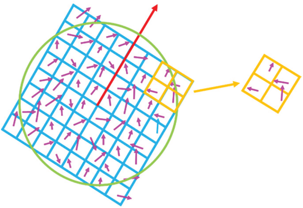
Figure 2: Orientation calculation by SURF

iii) Matching of Features

Considering the feature matching by SURF approach, the Euclidean distance parameter is utilized as the similarity measure for feature matching. The characteristic points of VA and VB feature points are given by DA and DB respectively. The distance between the two points is given by,

D(VA,VB)=∑i=1n⁡(DAi−DBi)2 (8)

In the feature matching process, the feature points are determined with the minimum and second minimum distance to the match point. The matching is considered as successful if the ratio of the minimum distance and the second minimum distance are lesser than the pre-set threshold.

2.4 Classification by Hybrid FF-GWO-CNN Algorithm

The classification process is carried out by the hybrid FF-GWO-CNN approach, which performs infusion of GWO into the FF algorithm. Generally, the FF algorithm is a renowned meta-heuristic approach related to the active flashing of fireflies. Depending on the firefly brightness, the best position for every particle is found by the FF algorithm, and the fireflies are regarded as unisex. In addition, the attractiveness of fireflies varies directly with the brightness, and this attractiveness lessens with the increase in distance. The expression for the intensity of light is given by,

I=Isexp(γh2) (9)

where h represents the distance between Is and fireflies, Is represents the light intensity of the source, and γ represents the absorption coefficient of the medium.

The brightness of fireflies is directly dependent on each other, which is given by,

β=β0exp(−γhm) (10)

where β indicates attractiveness.

Eq. (8) represents the distance between the ith and jth firefly and is given by,

hi,j=∑n−1k⁡(yi,n−yj,n)2 (11)

Due to increased attractiveness, the ith firefly moves towards the jth firefly and is represented by,

yi+1=yi+β0e−γhi,j2(yj−yi)+αε (12)

Although the FF approach mitigates the reduced attributes from high-dimensional data and minimises uncertainty and noise, it faces specific issues like unchanged parameters over time, holding less memory space and trapping in several local optima. Hence, the FF algorithm is incorporated with the GWO optimization approach. The functioning of GWO is dependent on the hunting nature of grey wolves. Parameters α,β and δ are the three groups of wolves assigned for hunting. The parameter α is the leader, which decides the hunting and sleeping time whereas, β and δ are the second best wolves helping α. Furthermore, ω is a redundant wolf group meant for only eating and is unimportant. Consider Yi as the population of grey wolves and the mathematical model related to the encircling nature of wolf is given by,

P=|U.XP(t)−X(t)| (13)

X(t+1)=XP(t)−V.P (14)

Here, U and V indicate the coefficient vectors, XP represents the position vector related to prey, X represents the position vector related to grey wolf, and t denotes the present iteration.

The formulation of U and V is given by,

V=2ar−a (15)

J=2r2 (16)

Here, r, r2 represent the random vector distributed uniformly along [0, 1], a indicates the component, which is diminished linearly from 2 to 0.

Mathematically, the hunting characteristics of the wolf are expressed by the following equations.

Pα=|U1Xα(t)−X| (17)

Pβ=|U2Xβ(t)−X| (18)

Pδ=|U3Xδ(t)−X| (19)

X1=Xα−V1Pα (20)

X2=Xβ−V2Pβ (21)

X3=Xδ−V3Pδ (22)

The wolf’s final updated position is expressed as,

X(t+1)=X1+X2+X33 (23)

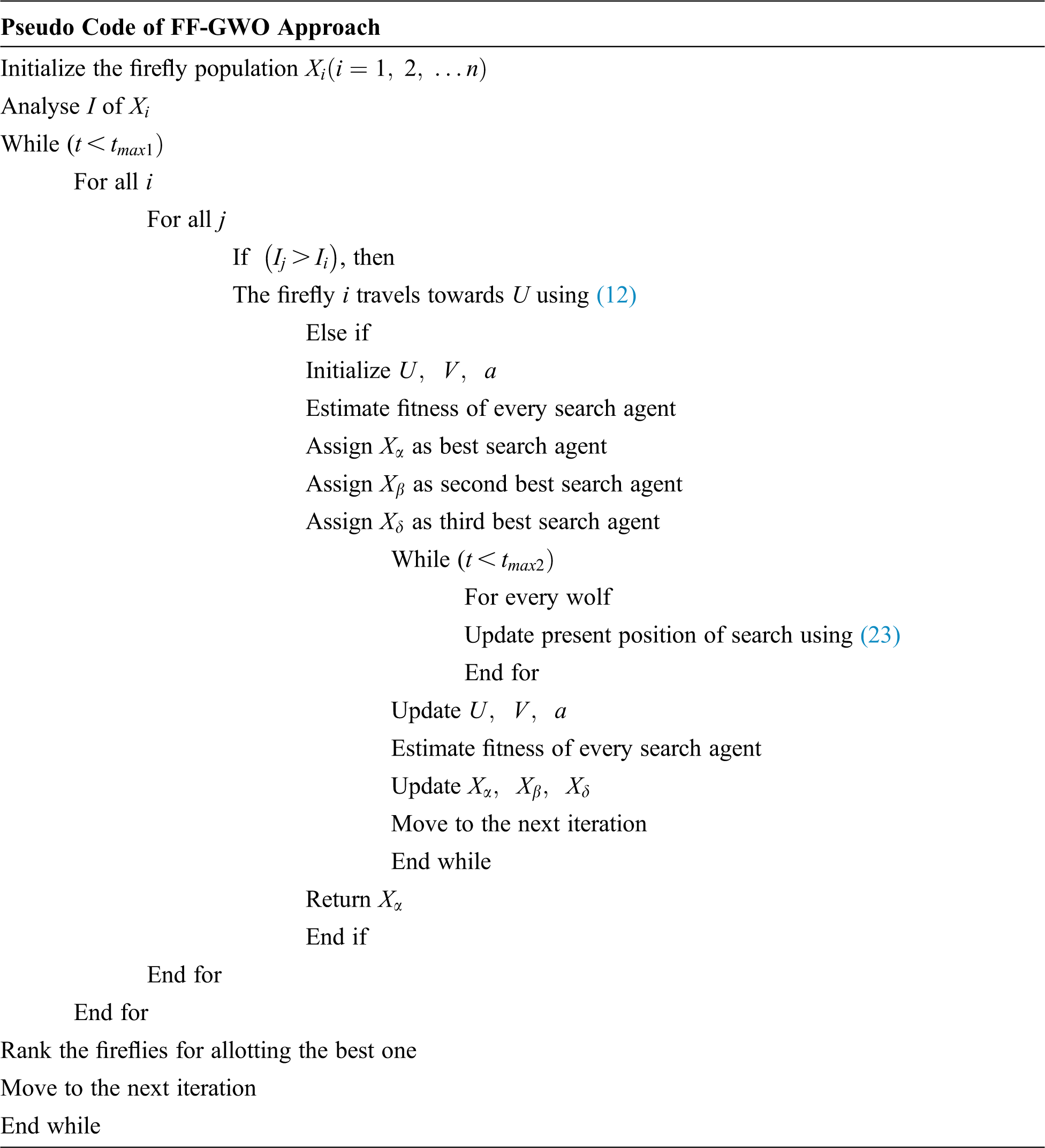
The pseudo-code for the FF-GWO approach is given below, and the corresponding flowchart is shown in Fig. 3.

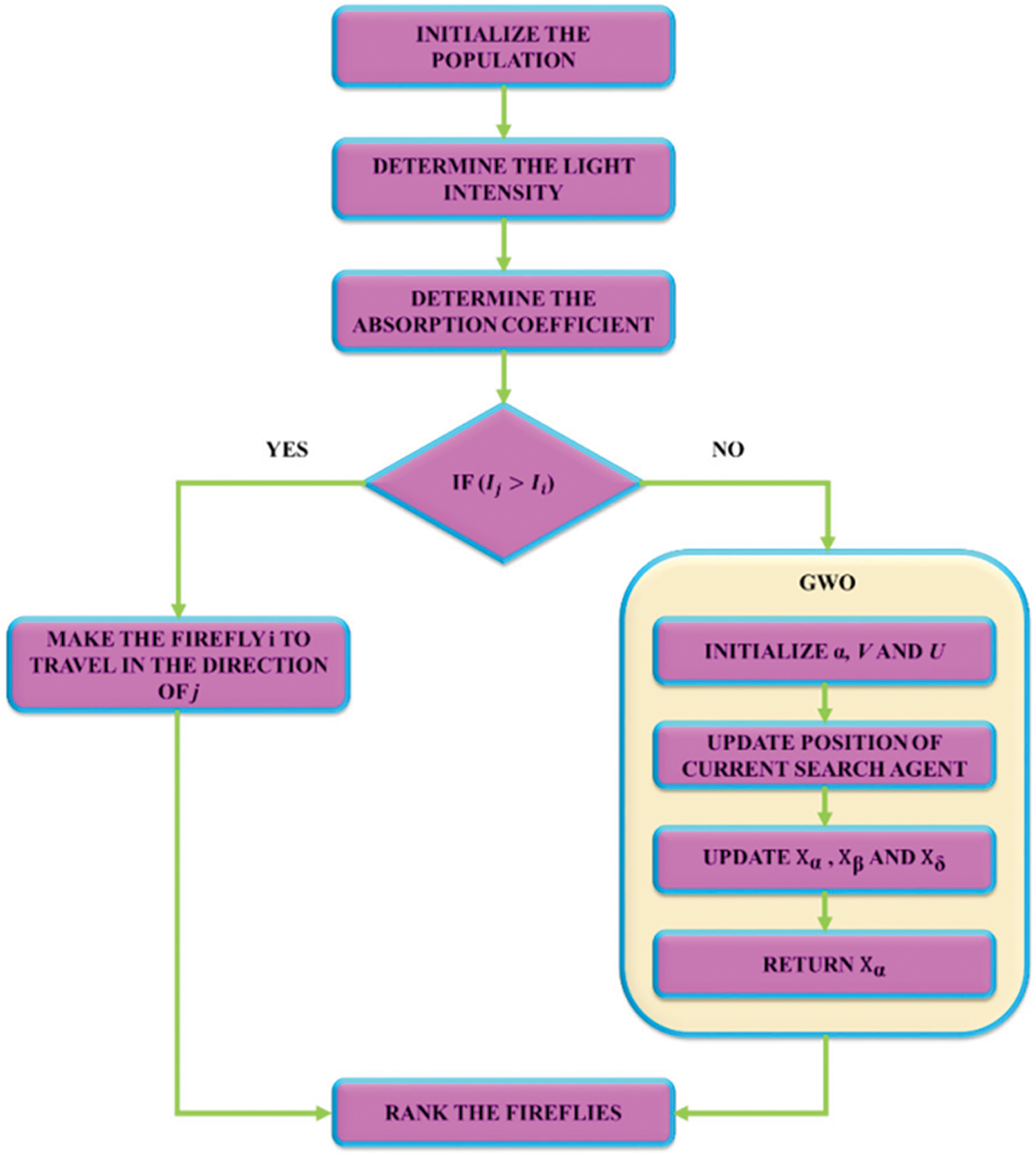
Figure 3: Flowchart for FF-GWO approach

In order to improve the accuracy of the classification process, FF-GWO is combined with CNN, which comprises an input layer, hidden layer and output layer, as shown in Fig. 4.

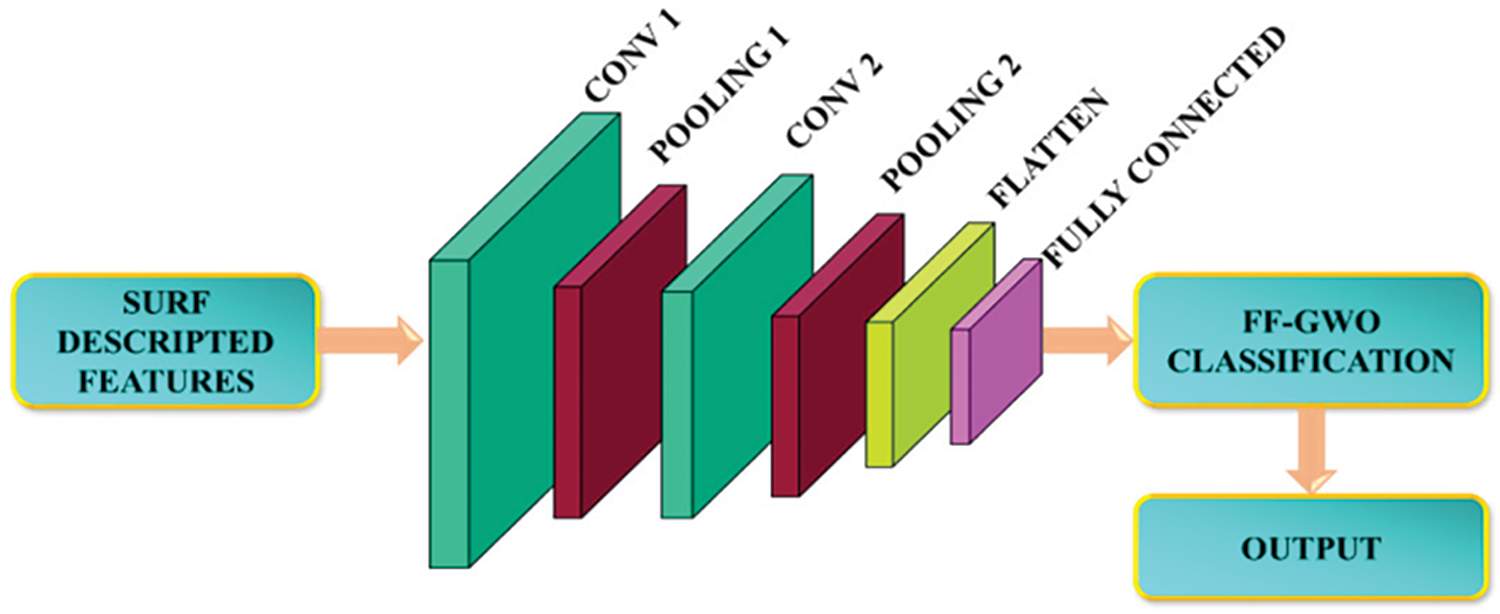
Figure 4: Proposed structure of CNN

CNN plays a significant part in image processing due to its advantages like increased model capacity and complex information obtained by the basic structural characteristics. Initially, a convolution core is defined in the convolution layer, and this convolution core is regarded as a local receptive field. During processing data information, the part of the feature information is extracted by the convolution core. The parameter sharing of convolution operation permits the network to learn a single set of parameters, which minimizes the parameter count and enhances the computational efficiency. The operation of convolution is expressed as,

pi,j=∑p=0h⁡∑q=0h⁡wp,qxi+p,j+q (24)

where, wp,q indicates convolutional kernel weight at p and q , h represents the height of convolutional kernel, xi,j indicates the image pixel value at i and j . Generally, the rectified linear unit (ReLU) is deployed as an activation function to avoid vanishing gradient and improve the training speed. The ReLU function is given by,

ReLU(y)={y,y>00,y≤0 (25)

Following the extraction of features, the neurons are fed to the pooling layer for the extraction of features again. The pooling layer maintains the feature map information to be more concentrated. Thus, it involves simplifying the computational complexity. The max pooling is generally utilized as a pooling layer and is given by,

Maxpool(H0,W0)={H0=floor((Hi+2p−k)s+1)W0=floor((Wi+2p−k)s+1) (26)

where, floor(x) indicates the function of round-up, H0 denotes the feature map output height, W0 indicates the feature map output width, Hi represents the feature map input height, Wi denotes the feature map input width, p indicates feature map padding, k denotes max pooling kernel size, s indicates max pooling kernel stride.

In the proposed CNN, two convolution layers, two pooling layers, a flattened layer, six hidden layers and a fully connected layer linked to the output layer are present. The convolution layers utilize 32 initial convolution filters adopting a kernel size of 6×6 . In order to attain an effective model of pest classification, the ReLU function is utilized for the activation of adjacent layer neurons. A pooling layer of 3×3 size is deployed next to each convolution layer in the absence of padding and has a stride of 2. Batch normalization is applied between the ReLU and convolution layer to increase the learning speed and classification accuracy. The fully connected layer has 2000 hidden nodes with a kernel size of 4×4 with valid padding. The data in the fully-connected layer is classified by FF-GWO approach, and the values are further transmitted to the output layer. The operational downsampling and the spatial dimensions are performed in pooling layer. The operation gets repeated based on the number of layers until the fully connected layer is reached. The performance of the CNN is evaluated by accuracy, recall, precision and F-measure. After completing the training process, the networks are exploited in the field to infer relevant results.

3  Results and Discussion

The proposed methodology is evaluated by using NBAIR, XIE and IP102 datasets with an image size of 3280 × 2464. These images are divided into a testing, training, and validation set. The obtained images are separated into 20% and 80% for validation and training, respectively, randomly. The testing set is also used at locations with the environment having possibly varieties of densities and variants of pests. The pest objects are cropped out after training.

Fig. 5 represents the input image, and Fig. 6 indicates the filtered image of the grayscale version obtained by the adaptive median filter. Fig. 7 indicates the separated foreground and background images. The foreground image indicates the image regions of higher priority with certain appropriate information and increased variations in space. It is further processed for attaining the binarized output. The background image, which is of reduced spatial variations, is usually not considered for processing. Initially, the background image is subjected to approximation and is eliminated.

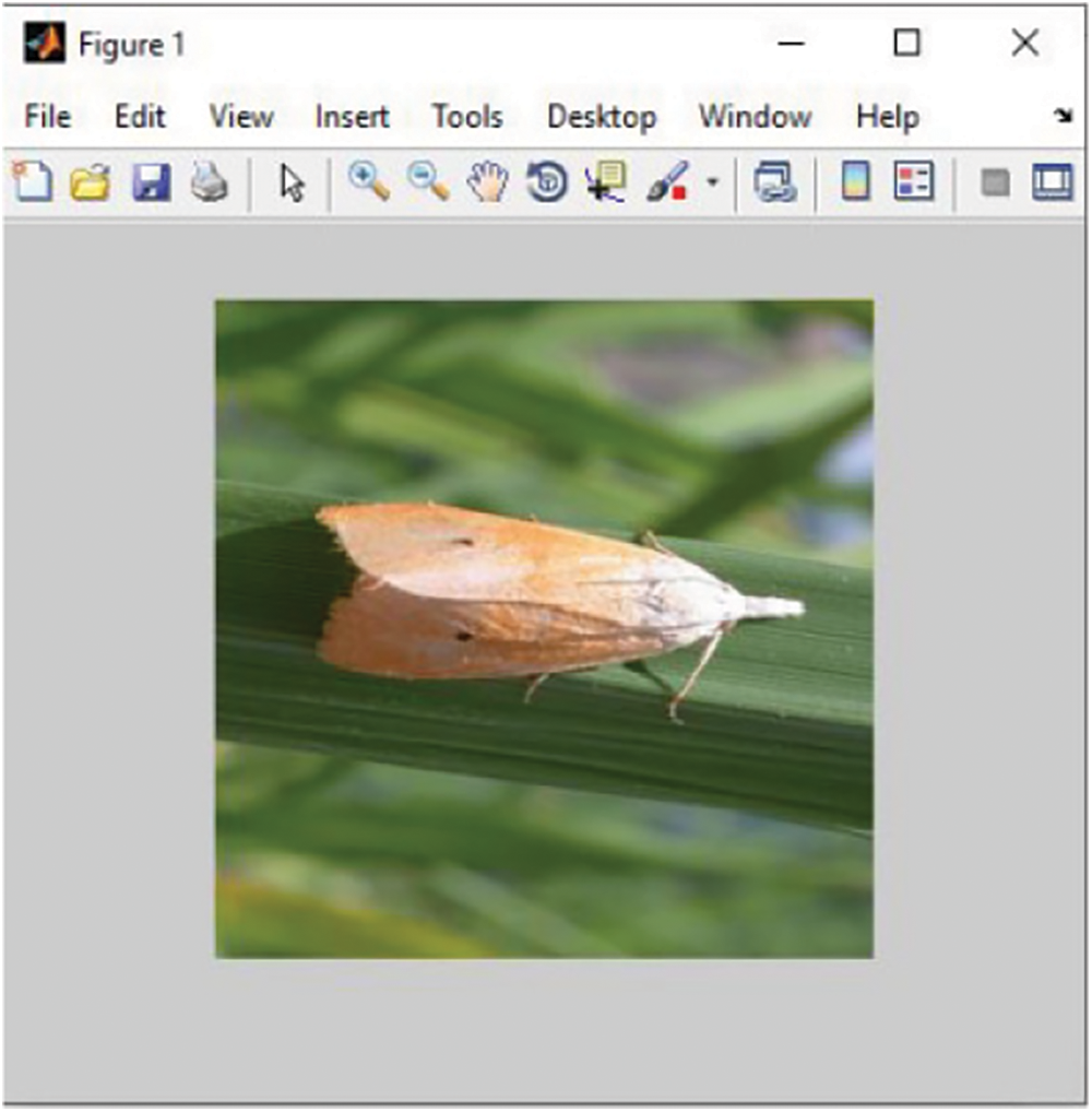
Figure 5: Input image

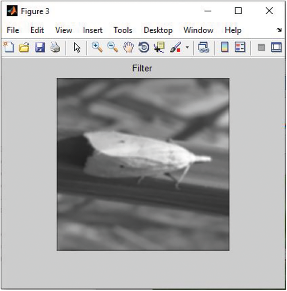
Figure 6: Filtered image

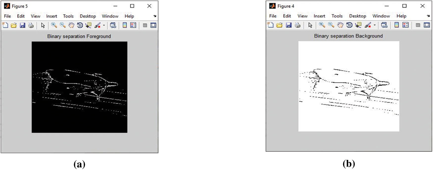
Figure 7: (a) Separated foreground image (b) Separated background image

Fig. 8 represents the segmented image by EMA utilizing a cluster number of 3. The clusters are segmented according to the brightness, and the obtained threshold value is equal to the mean value of brightest cluster. The segmented regions possess similar labels for the region of interest (ROI) and surrounding objects. Additional elements not associated with ROI are removed to obtain a clear image. A value of 1 is assigned to pixels with similar label values, and a value of 0 is assigned to keep label values.

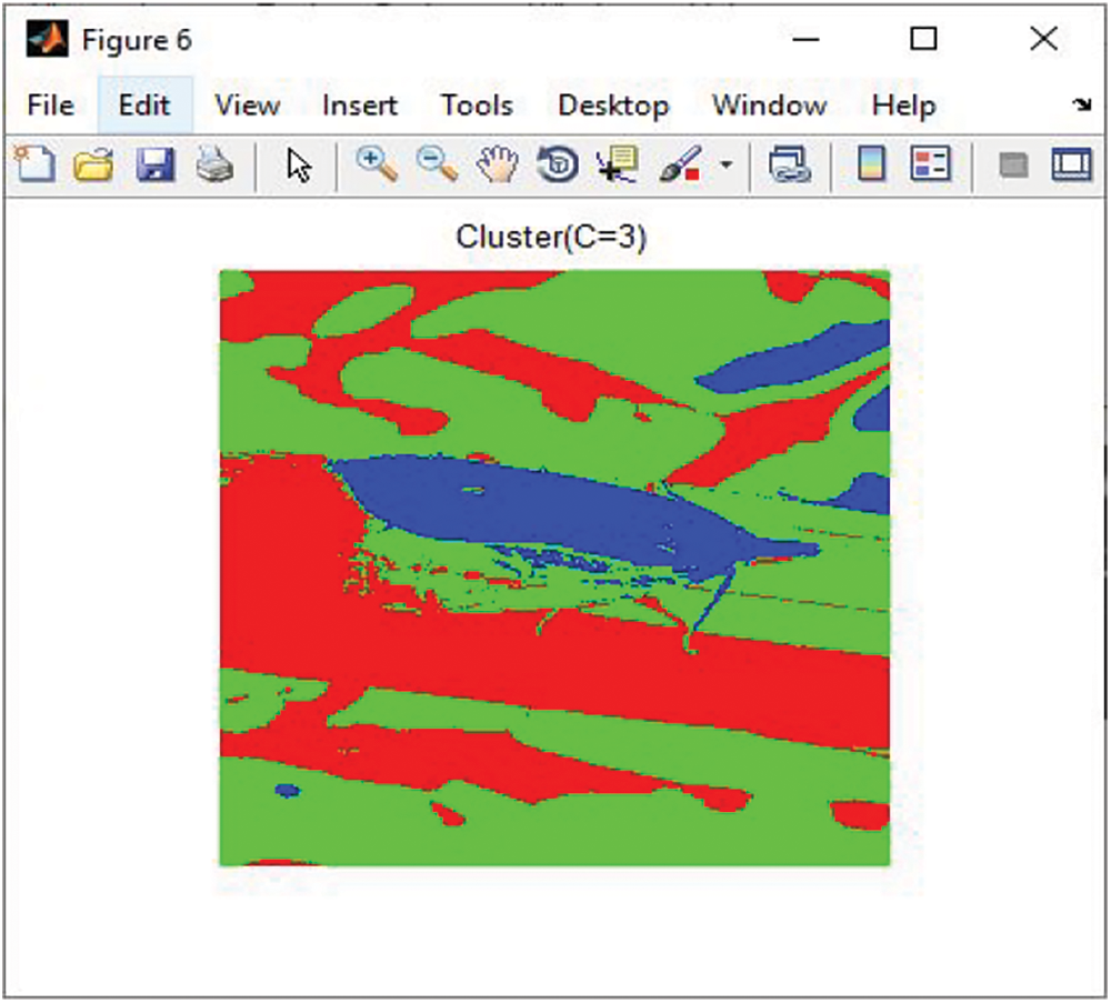
Figure 8: Segmented image

Fig. 9 indicates the descripted features, and Fig. 10 indicates the mapping of features. The performance of feature segmentation is assessed by detecting the total number of interest points. Generally, the SURF points are scattered across the image due to the wide feature shape variety detected by SURF approach. Regarding localization, SURF provides improved feature distribution and blob features detection.

Figure 9: Descripted features

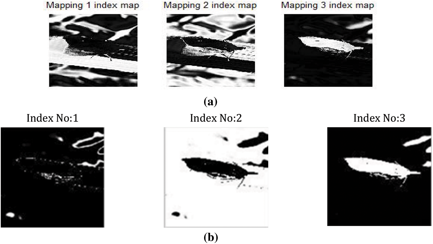
Figure 10: Mapping images

Fig. 11 represents the output generated by the proposed hybrid FF-GWO-CNN algorithm, and the obtained plots are as follows.

Figure 11: Generated output

Learning rate is a crucial factor for detecting the performance of the proposed approach. A high learning rate speeds up the learning process resulting in increased loss function and reduced learning rate. An optimized learning rate has to be selected to reduce the loss function for the detection of pests. This avoids the over-fitting issue and reduces errors. The results in Fig. 12 reveal that improved accuracy is attained at a learning rate of 0.0001.

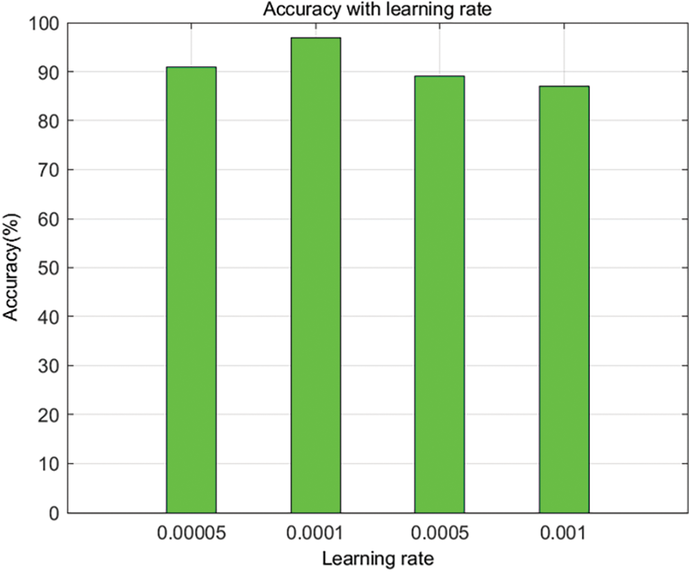
Figure 12: Value of accuracy with learning rate

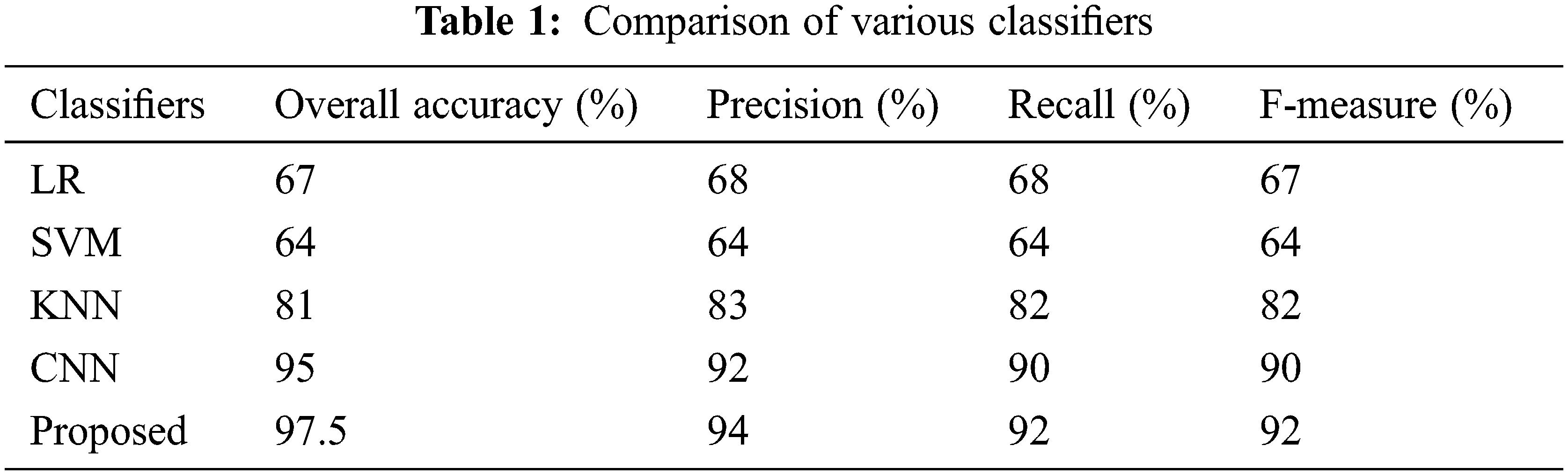
The mini-batch size is a crucial parameter influencing the accuracy, and increased batch size affects the performance. Hence, an appropriate mini-batch size is adopted. In this proposed approach, mini-batch sizes of 10, 16, 32, 64 and 128 are selected, as shown in Fig. 13. The obtained results depict that the accuracy shows a rapid increase for reduced mini-batch size. The comparison of obtained accuracy, precision, recall and F-measure with other conventional approaches is illustrated in Table 1.

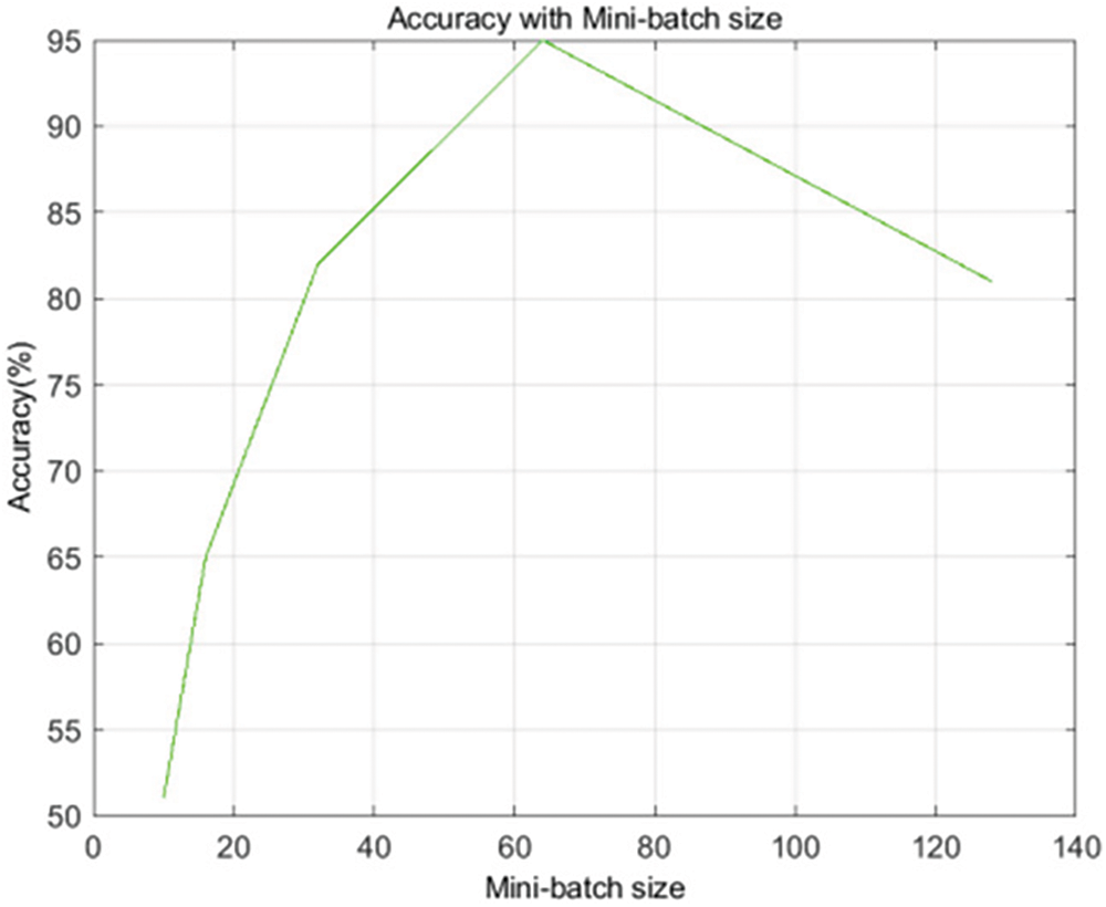
Figure 13: Accuracy variation with mini-batch size

Accuracy is considered a crucial factor and is estimated on the testing datasets at regular intervals. It is expressed as,

Accuracy=NumberofcorrectlypredictedinsectsOverallinputinsectsamples (27)

Precision and recall denote the balance between misdetection and false positive reduction. These parameters are expressed as,

Precision=TPFP+TP (28)

Recall=TPFN+TP (29)

Here, TP,FP,FN indicate True Positive, False Positive and False Negative, respectively. The precision estimates the incorrectly detected samples, and recall estimates mis-detected samples. F-measure combines the precision and recall values and is given by,

F−measure=2∗Precision∗RecallPrecision+Recall (30)

The experimental studies prove that the proposed pest detection approach based on image processing enhanced results with improved accuracy. The hybrid FF-GWO-CNN approach generates improved classification results with optimal outcomes.

The obtained outcomes of the comparative analysis are significantly illustrated through the graphical representation in Fig. 14, which proves that the proposed approach outperforms all the other existing approaches discussed in this study.

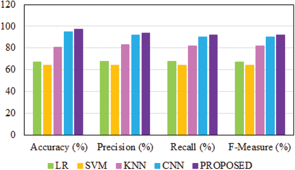
Figure 14: Comparative analysis

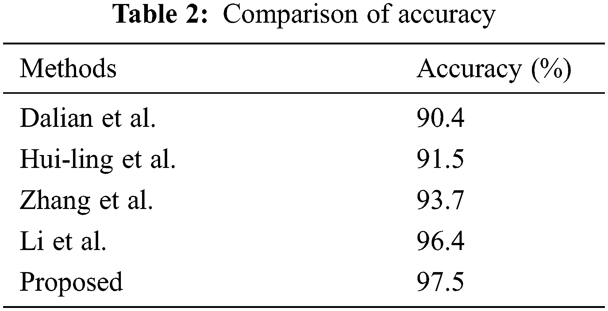
The accuracy of the proposed classifier is compared with some existing works of different authors, as shown in Table 2, which proves that the proposed classifier delivers more optimal accuracy than others.

4  Conclusion

The farmers are facing a massive difficulty in the early detection of pests in crops. In order to deal with this issue, various ways have been utilized. Manual inspection of large crop fields takes a long time and is inefficient. It also necessitates the presence of professionals, which makes it an extremely pricey operation. The image processing approach for pest detection in crops exhibits wide improvement prospects and enhanced potential to the traditional approaches. This paper utilizes an efficient image processing approach, in which an adaptive median filter carries out the pre-processing to provide enhanced visual clarity. The denoised image is further segmented by EMA, which provides improved accuracy. The segmented image undergoes a feature description approach by SURF, which is simple with minimized computation costs. Finally, CNN is used for classification, generating robust results with enhanced performance compared to pre-trained models. The proposed approach contributes to timely pest detection, avoiding crop damage due to harmful and toxic pesticides. Hence, it is validated that the proposed approach provides better performance with high accuracy of 97.5%, precision of 94%, recall of 92% and F-score value of 92%.

Acknowledgement: This work is supported by “Catalyzed and supported by Tamilnadu State Council for Science and Technology, Dept. of Higher Education, Government of Tamilnadu.”

Funding Statement: The authors received no specific funding for this study.

Conflicts of Interest: The authors declare that they have no conflicts of interest to report regarding the present study.

References

1. D. Abhishek, B. Debasmita and N. D. Kashi, “Automatic detection of whitefly pest using statistical feature extraction and image classification methods,” International Research Journal of Engineering and Technology, vol. 3, no. 9, pp. 950–959, 2016. [Google Scholar]
2. A. Fraser, “Land grab/data grab: Precision agriculture and its new horizons,” The Journal of Peasant Studies, vol. 46, no. 5, pp. 893–912, 2019. [Google Scholar]
3. S. M. Pedersen and K. M. Lind, “Precision agriculture—from mapping to site-specific application,” in Precision Agriculture: Technology and Economic Perspectives, 1st ed., Basel, Switzerland: Springer Nature, pp. 1–20, 2017. [Google Scholar]
4. L. Liu, R. Wang, C. Xie, P. Yang and F. Wang, “PestNet: An end-to-end deep learning approach for large-scale multi-class pest detection and classification,” IEEE Access, vol. 10, no. 7, pp. 45301–45312, 2019. [Google Scholar]
5. D. Xia, P. Chen, B. Wang, J. Zhang and C. Xie, “Insect detection and classification based on an improved convolutional neural network,” Sensors, vol. 18, no. 12, pp. 4169, 2018. [Google Scholar]
6. A. Fuentes, S. Yoon, S. C. Kim and D. S. Park, “A robust deep-learning-based detector for real-time tomato plant diseases and pests recognition,” Sensors, vol. 17, no. 9, pp. 2022, 2017. [Google Scholar]
7. K. Yamamoto, T. Togami and N. Yamaguchi, “Super-resolution of plant disease images for the acceleration of image-based phenotyping and vigor diagnosis in agriculture,” Sensors, vol. 17, no. 11, pp. 2557, 2017. [Google Scholar]
8. V. A. Natarajan, B. Macha and M. Sunil Kumar, “Detection of disease in tomato plant using deep learning techniques,” International Journal of Modern Agriculture, vol. 9, no. 4, pp. 525–540, 2020. [Google Scholar]
9. K. P. Ferentinos, “Deep learning models for plant disease detection and diagnosis,” Computers and Electronics in Agriculture, vol. 145, pp. 311–318, 2018. [Google Scholar]
10. M. Heenaye-Mamode Khan, N. Gooda Sahib-Kaudeer, M. Dayalen, F. Mahomedaly, G. R. Sinha et al., “Multi-class skin problem classification using deep generative adversarial network (DGAN),” Computational Intelligence and Neuroscience, vol. 2022, pp. 1–13, 2022. [Google Scholar]
11. K. K. Nagwanshi, “Learning classifier system,” in Modern Optimization Methods for Science, Engineering and Technology, IOP Publishing, Bristol, England, pp. 1–8, 2019. [Google Scholar]
12. D. Li, X. Wang, J. Sun and Y. Feng, “Radial basis function neural network model for dissolved oxygen concentration prediction based on an enhanced clustering algorithm and adam,” IEEE Access, vol. 9, pp. 44521–44533, 2021. [Google Scholar]
13. J. G. A. Barbedo, “A new automatic method for disease symptom segmentation in digital photographs of plant leaves,” European Journal of Plant Pathology, vol. 147, no. 2, pp. 349–364, 2017. [Google Scholar]
14. M. Mafi, H. Rajaei, M. Cabrerizo and M. Adjouadi, “A robust edge detection approach in the presence of high impulse noise intensity through switching adaptive median and fixed weighted mean filtering,” IEEE Transactions on Image Processing, vol. 27, no. 11, pp. 5475–5490, 2018. [Google Scholar]
15. J. Joseph and R. Periyasamy, “An image driven bilateral filter with adaptive range and spatial parameters for denoising magnetic resonance images,” Computers & Electrical Engineering, vol. 69, pp. 782–795, 2018. [Google Scholar]
16. W. Zhao, H. Lu and D. Wang, “Multisensor image fusion and enhancement in spectral total variation domain,” IEEE Transactions on Multimedia, vol. 20, no. 4, pp. 866–879, 2017. [Google Scholar]
17. S. H. Lin, P. Y. Chen and C. H. Lin, “Hardware design of an energy-efficient high-throughput median filter,” IEEE Transactions on Circuits and Systems II: Express Briefs, vol. 65, no. 11, pp. 1728–1732, 2018. [Google Scholar]
18. X. Qiu, M. Li, L. Zhang and X. Yuan, “Guided filter-based multi-focus image fusion through focus region detection,” Signal Processing: Image Communication, vol. 72, pp. 35–46, 2019. [Google Scholar]
19. V. N. Karnaukhov and M. G. Mozerov, “Fast non-local mean filter algorithm based on recursive calculation of similarity weights,” Journal of Communications Technology and Electronics, vol. 63, no. 12, pp. 1475–1477, 2018. [Google Scholar]
20. L. Deng, H. Zhu, Z. Yang and Y. Li, “Hessian matrix-based fourth-order anisotropic diffusion filter for image denoising,” Optics & Laser Technology, vol. 110, pp. 184–190, 2019. [Google Scholar]
21. A. C. Motagi and V. S. Malemath, “Detection of brain tumor using expectation maximization (EM) and watershed,” International Journal of Scientific Research in Computer Science and Engineering, vol. 6, no. 3, pp. 76–80, 2018. [Google Scholar]
22. L. Wan, T. Zhang, Y. Xiang and H. You, “A robust fuzzy c-means algorithm based on Bayesian nonlocal spatial information for SAR image segmentation,” IEEE Journal of Selected Topics in Applied Earth Observations and Remote Sensing, vol. 11, no. 3, pp. 896–906, 2018. [Google Scholar]
23. X. Tian, S. Fan, W. Huang, Z. Wang and J. Li, “Detection of early decay on citrus using hyperspectral transmittance imaging technology coupled with principal component analysis and improved watershed segmentation algorithms,” Postharvest Biology and Technology, vol. 161, pp. 111071, 2020. [Google Scholar]
24. L. Jiang, C. Xu, X. Wang, B. Luo and H. Wang, “Secure outsourcing SIFT: Efficient and privacy-preserving image feature extraction in the encrypted domain,” IEEE Transactions on Dependable and Secure Computing, vol. 17, no. 1, pp. 179–193, 2017. [Google Scholar]
25. H. Alhichri, A. S. Alswayed, Y. Bazi, N. Ammour and N. A. Alajlan, “Classification of remote sensing images using EfficientNet-b3 CNN model with attention,” IEEE Access, vol. 9, pp. 14078–14094, 2021. [Google Scholar]
26. Y. Li, H. Wang, L. M. Dang, A. Sadeghi-Niaraki and H. Moon, “Crop pest recognition in natural scenes using convolutional neural networks,” Computers and Electronics in Agriculture, vol. 169, pp. 105174, 2020. [Google Scholar]
27. N. Baghel, U. Verma and K. K. Nagwanshi, “WBCs-Net: Type identification of white blood cells using convolutional neural network,” Multimedia Tools and Applications, pp. 1–17, 2021. https://doi.org/10.1007/s11042-021-11449-z. [Google Scholar]
28. M. Heenaye-Mamode Khan, N. Boodoo-Jahangeer, W. Dullull, S. Nathire, X. Gao et al., “Multi-class classification of breast cancer abnormalities using deep convolutional neural network (CNN),” PLoS One, vol. 16, no. 8, 2021. https://doi.org/10.1371/journal.pone.0256500. [Google Scholar]
29. S. K. Rajesh Kanna, V. Nagaraju, D. Jayashree, A. Munaf and M. Ashok, “A maize crop yield optimization and healthcare monitoring framework using firefly algorithm through IoT,” Artificial Intelligence and Data Mining Approaches in Security Frameworks, pp. 229–245, 2021. https://doi.org/10.1002/9781119760429.ch13. [Google Scholar]
30. C. Chen, X. Wang, H. Chen, C. Wu, M. Mafarja et al., “Towards precision fertilization: Multi-strategy grey wolf optimizer based model evaluation and yield estimation,” Electronics, vol. 10, no. 18, pp. 2183, 2021. [Google Scholar]
Cite This Article
Copyright © 2023 The Author(s). Published by Tech Science Press.
This work is licensed under a Creative Commons Attribution 4.0 International License , which permits unrestricted use, distribution, and reproduction in any medium, provided the original work is properly cited.
Downloads
Citation Tools