Leaching Fraction (LF) of Irrigation Water for Saline Soils Using Machine Learning

1  Introduction

Soil salinity is the accumulation of salts in soil due to the natural material of soil or due to poor agronomic practices [1]. This soil salinity is a serious threat to sustainable agriculture development [2]. To deal with the issue of soil salinity, extra irrigation water is applied to leach down the salts from the root zone of the plants. Leaching is the process of application of irrigation water to percolate down the salts from the root zone of the plants. LF is the ratio of irrigation water required to leach down the salts to a specific level of soil salinity. The application of irrigation water for leaching purposes without calibration according to environmental conditions usually fails to reduce soil salinity effectively [3].

To effectively achieve the objective of leaching, the irrigation water used for leaching purposes must be adjusted to environmental conditions and salinity levels. To adjust the LF according to the environmental conditions the LF is adjusted with the Evapotranspiration (ET) rate. ET rate is the measure of water loss from the soil and plant surface in the form of evaporation and transpiration, collectively called ET [4]. Reference Evapotranspiration (ETo) is used to model the ET rate of a model crop. ETo is the standard ET of the grass crop [5]. The ET of the model crop (grass) is called Reference ETo. The ETo rate is heavily affected by the temperature, humidity, wind speed, and sunshine duration. The ET rate increases with temperature and decreases with an increase in humidity [6].

ET is affected by environmental conditions with a severe impact on LF to be available for an effective leaching process. Irrigation must be adjusted with the ET rate to ensure the LF of irrigation water is available under prevailing environmental conditions. Many methods of ETo rate determination are recommended. Most important are Blaney Criddle, Penman Montieth method, and Pan Evaporation method [7].

These methods required a lot of parameters that make them difficult to apply at the farmer level. LF of irrigation water applications without adjustment to the prevailing conditions usually fails to achieve the objective of leaching in saline soils. Leaching is applied without any calibration according to the salinity level and environmental conditions. Leaching irrigation water needs to be calibrated according to the environmental context, to successfully reduce the soil salinity by the leaching process. The failure in the leaching process results in loss to the farmers. LF is the fraction of total irrigation water required to reduce soil salinity from a certain salinity level to the desired salinity level.

Machine learning has revolutionized the world by transforming all spheres of life including healthcare, agriculture, transport, entertainment, and business. ML is also applied in agriculture to deal with different problems in agriculture. Many ML-based solutions were proposed to determine the ET rate from limited environmental conditions. Determination of LF from ML-based ETo rate is not previously targeted. To determine the LF from limited environmental conditions the ML model is proposed to determine the calibrated Evapotranspiration (ETc) from the prevailing temperature, humidity, and sunshine duration. To train and validate the Model the Blaney Criddle Method of ET rate determination is used. Many smart irrigation water solutions were proposed in recent years for the conservation of irrigation water. Most of the proposed solutions were limited to sensing soil moisture conditions and recommendations for the irrigation water accordingly. Very few smart irrigation water solutions follow Food and agriculture organization (FAO) recommended method of ET for the determination of irrigation water requirements [8].

1.1 Significance of Study

Soil salinity has a profound impact on the socio-economic life of people. Soil salinity has seriously affected more than 831 million hectares of land, across the world [9]. Soil is a non-renewable resource that is very important to feed the ever-increasing population. Every sphere of knowledge should focus to reclaim the saline soil. Soil salinity is a significant environmental hazard that affects crop yield and production. Soil Salinity is the primary source of reduction in crop yield and source of barren soil [10]. A high concentration of salt affects the plant’s ability to uptake the water [11].

Due to progressive human-induced salinization, the soil at an alarming rate has become unsuitable for agricultural and infrastructure developments [12]. Poor agriculture practices are the primary reason for human-induced soil salinity. Salinity is a severe problem in irrigated areas and results in considerable loss to the value of production [13]. Soil salinity is an issue in more than seventy countries. Soil salinity cause 1%–2% of land degradation per year. Around 20% of irrigated land is affected by soil salinity [14].

Soil salinity is the major problem in arid regions that causes severe economic losses to the farmers. The soil salinity is very toxic to plants. Most of the plants cannot survive in saline culture. The salts uptake by the plants interferes with the normal physiology of the plants. The toxicity of salinity results in the death of the plants which causes severe loss to the farmers. To feed the ever-increasing human population. Every sphere of knowledge must contribute to dealing with issues. The proposed solution intends to improve the effectiveness of the leaching process to reduce soil salinity. The reclamation of saline soils for agriculture purposes by effective leaching would save the most precious resource.

1.2 Contribution

The major contribution of the work is the determination of the LF of irrigation water to deal with the issue of soil salinity efficiently and effectively. The proposed solution optimizes the use of irrigation water for leaching purposes according to environmental conditions (temperature, humidity, wind speed) that were not previously targeted. The relationship between environmental conditions and ET is diverse.

Some conditions tend to increase the ET, and some decrease the ET rate. The combined effect of all the environmental conditions is hard to determine from the linear model. Therefore, ML-assisted ETo rate is determined to optimize the LF according to the environmental conditions. LF determination from limited environmental conditions aims to support sustainable developments in agriculture.

1.3 Data-Driven Machine Learning Model

A data-driven machine learning model is applied to make decisions for the smart LF of irrigation water. The proposed solution is ideal for dealing with the issue of soil salinity while conservation of irrigation water, to support sustainable developments in agriculture. The proposed solution aims to effectively deal with the issue of soil salinity by smart leaching of irrigation water. Smart leaching fraction of irrigation water application according to the prevailing, temperature, humidity, wind speed, and sunshine duration can effectively deal with the issue of soil salinity in irrigated areas.

2  Literature Review

The literature review is performed to find relevant work, from major bibliographic indices. Many solutions regarding smart irrigation have emerged in recent years. Hellin et al. presented an automated smart irrigation Decision Support System for smart water conservation [15]. Olivo proposed an automated actuator for the control of irrigation water according to environmental conditions [16]. Rojo proposed irrigation water requirements by observing the stress in the leaf of plants [17]. El-Kader reviews the Wireless sensor network (WSN) applications in agriculture for precise use of the resources especially the irrigation water [18].

Mulenga et al. recommended irrigation water conservation techniques by applications of irrigation water according to the prevailing environmental conditions [19]. Haghverdi et al. [20] recommended site-specific irrigation according to the level of soil moisture in the field. Mohanraj et al. [21] proposed irrigation water requirements by sensing environmental conditions from the crop field.

Gutierrez et al. proposed optimized irrigation water requirements for precise estimation of irrigation water according to the environmental conditions [22]. Nikolidakis et al. proposed automated irrigation water management according to prevailing environmental conditions [23]. Sales et al. proposed automated irrigation using sensors to sense the environmental conditions [24]. Garcia et al. proposed site-specific irrigation water management in crop fields [25]. Xie et al. proposed irrigation water management using a fuzzy programming approach [26].

Feng et al. recommended an ML-based ET determination method from environmental conditions [27]. Ilic et al. recommended an efficient irrigation water schedule using a neuro-fuzzy approach [28]. Coates et al. proved an automatic valve for irrigation water management [29]. Gocic et al. suggested ML-assisted ET rate determination based on temperature data of a location. [30].

Goumopoulos et al. proposed irrigation water requirements for plants using the “speaking plant” approach [31]. Kong et al. recommended a technique to assess the soil moisture conditions for irrigation water recommendations [32]. Karim et al. recommended irrigation water conservation using the WSN [33]. Ramachandran, et al. recommended crop irrigation water requirements according to the prevailing environmental conditions [34]. Afrasiabikia et al. [35] recommended a distribution system of irrigation water to prevent losses of irrigation water. Shi et al. reviewed the recent developments of IoT applications in protected agriculture [36]. Ahmed et al. recommended smart farm architecture [37].

Popovic et al. recommended IoT infrastructure for ecological monitoring [38]. Rajalakshmi et al. proposed IoT crop field monitoring for the irrigation water recommendation. Talavera et al. [39] explored the IoT application in agriculture. Naqvi et al. recommended IoT-based irrigation management applications to conserve irrigation water [40]. The study in [41] proposed leaching estimation in saline soil with temperature conditions of an area. Wang et al. [42] evaluate the remote sensing, machine learning and Land surface model (LSM) based approaches where results indicate that ensemble means of global terrestrial ET rates are similar in all the approaches.

Niaghi et al. [43] proposed ML-based ETo, estimation in humid conditions due to the non-linear characteristics of the ETo determination. The ML models [44] are compared in terms of RMSE, MAE, Scattered index (SI), and Co-relation coefficient. It is observed that the RF model is more accurate in ETo estimation with radiation as input. Faramiñan et al. [45] proposed daily actual Evapotranspiration (ETa) of barley crops by the development of the linear generalized model, developed from meteorological conditions.

López et al. [46] proposed ETo estimation with soil moisture conditions using the regression model. The proposed solution determines the crop potential Evapotranspiration (ETc) of Kikuyu grass. The Eto by proposed solution is compared against the Penman Montieth method. The model achieved a coefficient of determination of 0.9936, with RMSE 0.183 mm day−1. Allen et al. [47] recommended weather data conditioning to deal with the problem of overstated ETo to adjust biases in ordinary conditions, especially in arid conditions.

Martínez et al. [48] evaluated the performance of Remote sensing (RS) based ETo estimation at low altitudes. The study evaluated the performance of MODIS ET (MOD16), Global land evaporation amsterdam model (GLEAM) ET, and Atmosphere-land exchange inverse (ALEXI) ET. Petkovic et al. [49] recommended a regression model of ETo determination from several weather conditions. Wang et al. [50] proposed radiation-based ETo estimation from RS data considering the complex terrain. The implementation of the proposed result yields that R2 is 0.84 and 0.86 at two different locations with 0.59 and 0.82 RMSE respectively.

Ma et al., [51] suggested an ET estimation framework from high-resolution RS data from Sentinel-2 satellite data. The coefficient of determination of the proposed solution is from 0.870 to 0.912 mm day−1. The coefficient of determination of the proposed solution is from 0.870 to 0.912 mm day−1.

Many ML-assisted solutions were proposed to determine the ETc rate from prevailing environmental conditions. Recommendation of LF based on ET rate from limited environmental conditions is not previously targeted. The proposed solution would support sustainable developments in agriculture with the reclamation of saline soils with an effective leaching process with the conservation of irrigation water.

3  Materials and Methods

The smart LF of irrigation adjusts the ET rate with environmental conditions using the ML approach. Initially, the ETc rate was based on temperature, humidity, and sunshine duration. LF of Irrigation water is determined using the ET rate and salinity level of the soil and irrigation water of the crop field. LF is used to determine the fraction of total irrigation water that is required to reduce salinity up to the target level of soil salinity. LF and ETc are used to determine the irrigation water requirements according to the temperature, humidity, wind speed, sunshine duration, and prevailing salinity conditions.

3.1 Flow Chart of Proposed Method

The proposed solution determines the ETo from the temperature and day length of an area using the Blaney Criddle method of ET. Blaney Criddle is a theoretical measure of ET rate and ignores the impact of humidity, sunshine, and wind speed. ML model is used to determine calibrated ETc rate according to humidity, sunshine, and wind speed. ETc and LF are used to determine the total irrigation Water requirements (WR).

3.1.1 Blaney Criddle Method of Reference Evapotranspiration (Et0)

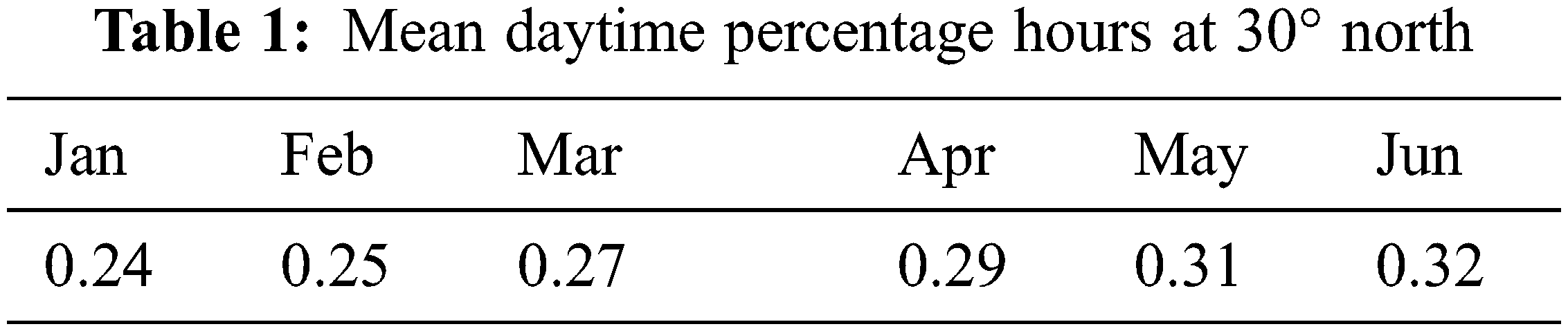
ETo is the ET rate of reference crop in millimeters in one day (mm day−1). It is obtained by using the Blaney-Criddle method, by Eq. (1), where ‘Tmean’ is the mean monthly temperature, and ‘p’ is the daily percentage of daytime in hours.

ETo=p(0.46×Tmean+8) (1)

The daytime length has a significant impact on irrigation requirements and ET rate. The experiment area is situated at the latitude of 30° N. Value of daytime length ‘p’ is taken from the mean daytime percentage hours based on latitude and month. Table 1, shows the “p” value of the experiment area (Vehari, Pakistan) for January to June.

Tmean is the mean monthly temperature obtained by mean monthly maximum temperature (Tmax) and means monthly minimum temperature (Tmin) by Eq. (2).

Tmean=(Tmax+Tmin)2 (2)

Tmax is obtained by Eq. (3), where ‘n’ is the maximum number of days in a month, and Tx is the maximum daily temperature.

Tmax=SumofmaximumtemperatureNodaysinonemonth=∑i=1n⁡Txin (3)

Tmin is obtained by Eq. (4), where ‘n’ is the number of days and Tn is the minimum daily temperature. All these temperature measurements are made on a degree centigrade scale (°C).

Tmin=SumofminimumdailytemperatureNodaysinonemonth=∑i=1n⁡Tnin (4)

The flow chart of the method is given in Fig. 1. Start the process where the mean monthly temperature and daylight tends to ET0. Average monthly sunshine, humidity, and wind speed lean towards ETc. Finally, the crop tolerance level, irrigation water salinity, and soil salinity measure the leaching fraction. Then this whole process calculates the total requirement of water before the end.

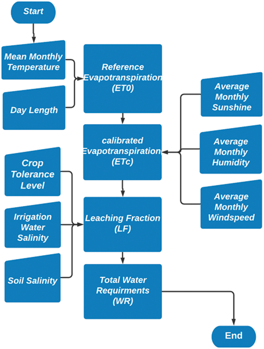
Figure 1: Flow chart of the proposed solution

3.1.2 Leaching Fraction (LF)

The LF is the fraction of irrigation water required to control salinity within the crop tolerance level. LF of irrigation water is determined according to the soil salinity, irrigation water salinity, and crop tolerance The LF is expressed by Eq. (1), where ‘ECw’ is the irrigation water salinity level in dSm−1, and ‘ECe’ is the salinity tolerance level of the crop. ‘ECe for the grass crop at one-hundredth percent (100%) of yield potential is 8.7.

LF for the grass crop with a tolerance level of 8.7 dSm−1 is determined by the FAO recommended method by Eq. (5).

LF=ECw/(5(ECe)−ECw) (5)

The Water requirements in the experiment area (WRe) are calculated by Eq. (6), where ETc is the calibrated Evapotranspiration (ETc) and LF is determined by Eq. (5).

WRe=ETc/(1−LF) (6)

For comparison purposes, the Water requirements in the control area (WRc) are obtained by using the ET0 from the Blaney Criddle method by Eq. (7). The WRc is applied in the control area and WRe is applied in the experiment area to observe the effectiveness of both solutions.

WRc=ETo/(1−LF) (7)

The theoretical ET0 by Blaney Criddle method ignores the impact of humidity, wind speed, and sunshine duration on ET rate. ML-assisted smart ETc rate is determined according to the prevailing humidity level, wind speed, and sunshine duration. The objective of the ML model is to effectively adjust the ET0 according to humidity, wind speed, and sunshine duration ratio.

The dataset for the ML is obtained by conditions shown in Fig. 2 and by the Blaney Criddle method. Each line shows the ETc according to the humidity, wind speed, and sunshine. The ETc is calibrated according to these conditions. The ideal outcome of the model would be the minimum amount of irrigation water that serves the irrigation water requirements for LF to be successfully available. The success matric in this regard would be the smart calibrated irrigation water according to the environmental conditions.

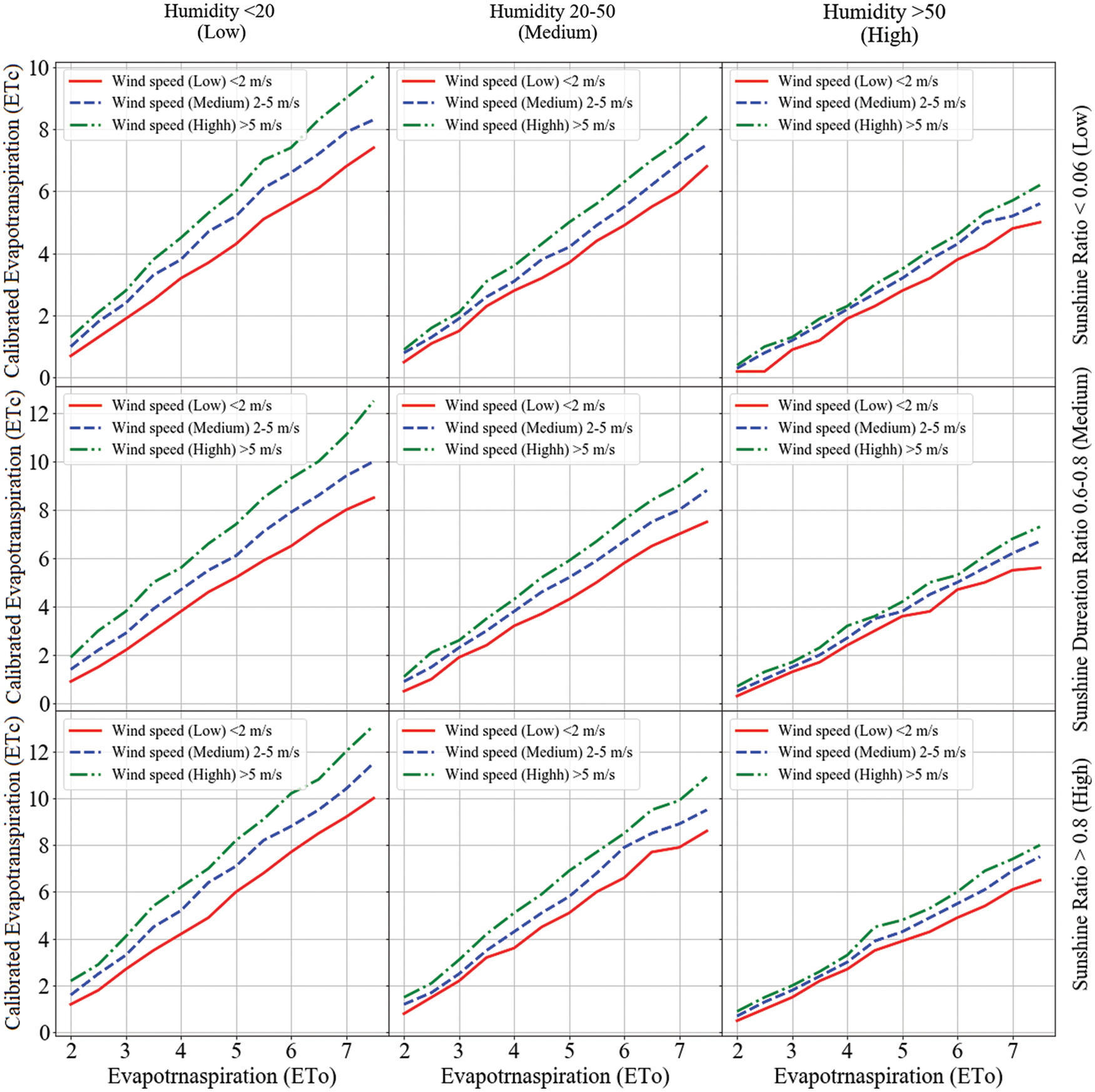
Figure 2: Machine learning data set [6]

The model is deemed to be a failure if the recommended irrigation water fails to achieve the objective of leaching. The input to the model would be the ETo, humidity, wind speed, and sunshine duration. Fig. 2, shows the environmental data for ML training.

The ML model is developed using multiple regression. The regression model is used due to the existence of the linear relationship between environmental conditions, ETc. The training of the model is done with more than one hundred thousand records. Eighty percent (80%) of the data set is used for the training of the model and twenty percent (20%) for the test data set.

The objective of the model is to directly predict the ETc from the direct values of humidity, wind speed, and sunshine duration. Fig. 3, shows the distribution of the data of ETc in the test data set.

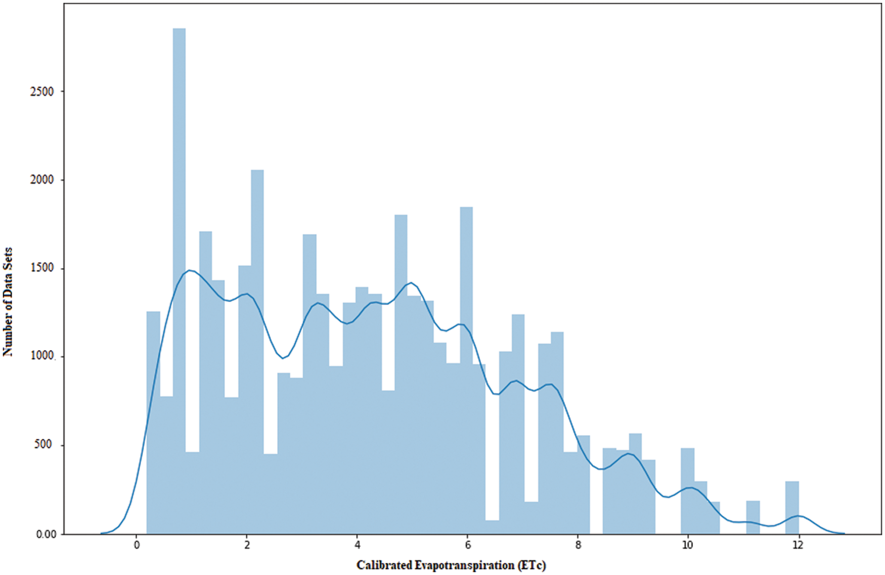
Figure 3: Distribution of Etc in the test data set

3.1.3 Machine Learning (ML) Model

4  Results and Discussion

This section intends to evaluate the proposed method of smart LF of irrigation water with different prospects. Initially, the performance of the ML model is made with different types of evaluations. The performance of smart LF of Irrigation water is compared against the traditional method of LF of Irrigation water.

4.1 Performance of Machine Learning Model

The proposed ML model predicts the ETc from the humidity, wind speed, and sunshine as the input to the model. The performance of the model is observed in terms of the accuracy of the model to determine the calibrated ETc. The ETc predicted by the proposed solution is compared against the Blaney Criddle of ET rate determination to find the difference in prediction. The difference in predicted and actual ET values from the test data set is shown in Fig. 4.

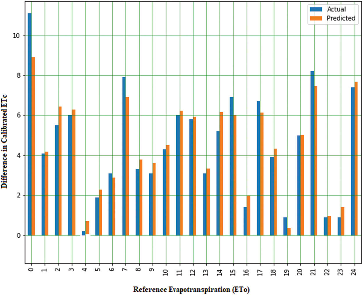
Figure 4: The difference in actual and predicted ET

For the different levels of ETo, the difference in calibrated ET (ETc) is shown in Fig. 4. For each case, the difference is very low. The maximum difference is 2 mm day−1 and the minimum difference is 0.2 mm day−1 for all observed ETc values. For most of the observed values, the difference is less than 1 mm day−1. The difference in calibrated ET (ETc) is low against each set of ETo.

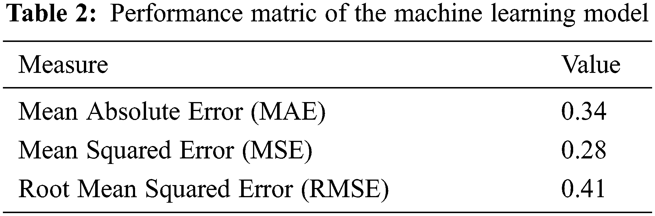
The performance of the ML model is observed in terms of mean absolute errors (MAE), Mean squared errors (MSE), and Root means squared errors (RMSE). The MSE is the average of the Squared Errors. MSE is the average of the square of the difference between the predicted values and actual values. MSE is expressed by Eq. (8), where ‘n’ is the number of observations. It is the measure of the distance of points from the regression line.

MSE=1n∑⁡(Actual−Predicted)2 (8)

Root Mean Squared Error (RMSE) is the square root of the average of the MSE. RMSE expressed by Eq. (9), is related to an estimator.

RMSE(∅)=MSE(∅)=1n∑⁡(Actual−Predicted)2 (9)

Mean Absolute Error (MAE) is the average of the difference between the observed value and actual value measured using the same phenomenon. MAE is expressed by Eq. (10), where ‘Yi’ is the observed value of the ‘ith’ item and ‘xi; is the actual value of the ith item.

MAE=∑i=1n⁡|yi−xi|n (10)

In Table 2 the value of MAE 0.34, MSE 0.28 and RMSE 0.41 in mm day−1 are low against the test dataset of the model, which reflects the accuracy of the model in making Etc prediction. The test data statistics show that the ML model is accurate in the prediction of ETc against the prevailing environmental conditions. The proposed model can be used with accuracy and confidence in the estimation of irrigation water requirements from the LF, ETc.

4.2 Field Effectiveness of Smart Leaching

The effectiveness of the proposed smart LF of irrigation water is also observed by the application of the proposed solution in a real-time environment. The effectiveness of the proposed solution is compared to the traditional leaching process. To implement and compare the performance of both leaching processes is applied in two adjacent areas with similar soil salinity levels. In the experiment area, the leaching process is applied according to the proposed solution while in the control area the leaching process is applied by the traditional process. In both areas, the salinity level is observed before and after leaching water application.

The salinity is observed before and after the application of leaching irrigation water in both areas. In both areas, salinity is observed at sixty-four sampling points for soil salinity in terms of electric conductivity (EC). The impacts of leaching by the smart and traditional methods are analyzed in terms of average soil salinity ECav. The average soil salinity (ECav) is determined by Eq. (11), where ‘n = 64’ is the total number of sample points, ‘i’ is the sample point number, and ‘EC’ is the EC value at the sampling point. The targeting tolerance level is set for the cotton crop that is 8.7 dSm−1 or below.

ECav=∑i=1n⁡ECi (11)

4.2.1 Salinity Distribution Before Leaching

Initially, the soil salinity is observed in both the control and experiment areas before the application of irrigation water for leaching purposes.

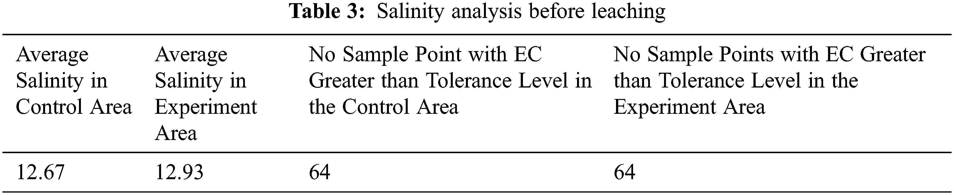
In Fig. 5, the salinity distribution of both experiment and control areas is plotted before the application of irrigation water for leaching purposes. Before the leaching process, the ECav in the control area was 12.67 dSm−1, and in the experiment, the area was 12.93 dSm−1. In both areas, salinity at all the sixty-four (64) sample points was higher than the tolerance level of the selected crop which is 8.7 dSm−1. Both areas have similar ECav, and at all the sample points the salinity is above the tolerance level of the crop as given in Table 3.

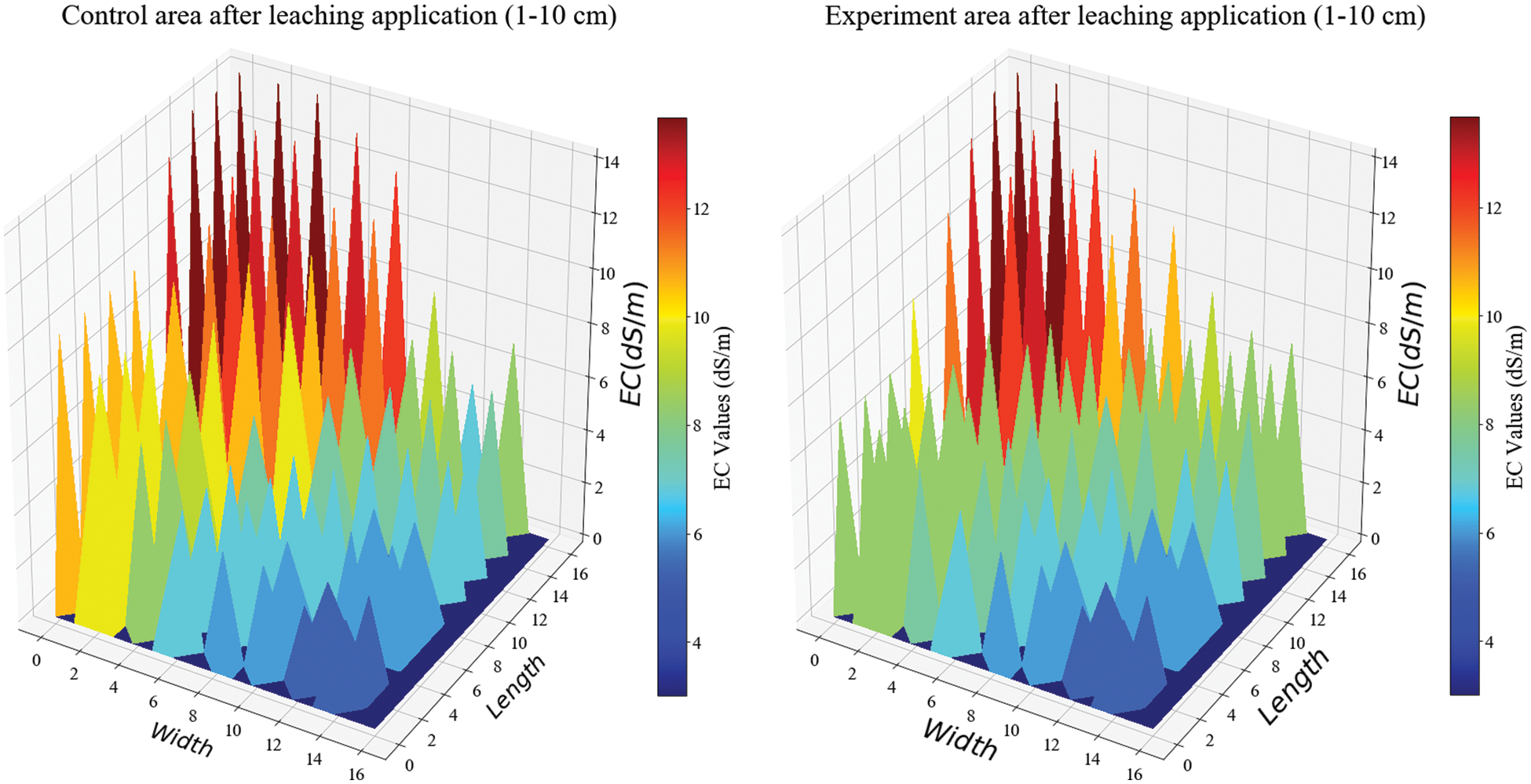
Figure 5: Soil salinity distribution after leaching application

4.2.2 Salinity Distribution After Leaching

The WRe are determined based on ETc and LF. The smart calibrations in ETc are made based on crop field environment conditions. The WRe is determined by predicted ETc of 5.3 mm day−1. With irrigation water salinity of 5 dSm−1 and a targeted level of soil salinity of 8.7 dSm−1, the required LF is 0.13 determined by Eq. (5). It means thirteen percent (13%) more irrigation water is required to serve the objective of leaching. With ETc of 5.3 mm day−1, the total requirements of irrigation water would be 6.23 mm day−1, with LF of 0.13. While in the control area the WRc, is applied with the traditional method by applying Eq. (7).

Soil salinity distribution is compared in both the control and experiment area after leaching application. Salinity distribution after the application of WRe and WRc in the control and experiment area is shown in Fig. 5. Salinity distribution in the experiment and control area is given in Table 4.

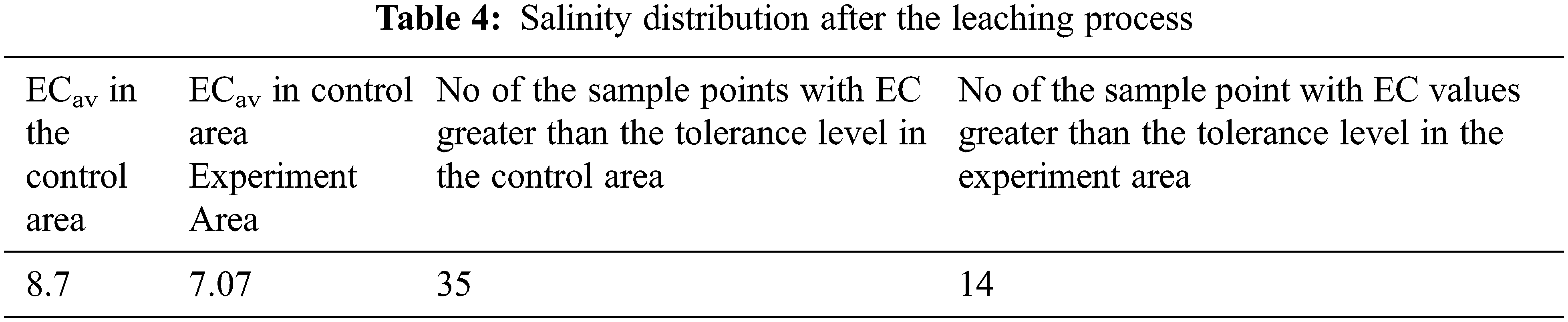
In the experiment area, the ECav is 7.07 dSm−1, and in the control, the area is 8.7 dSm−1. In the control area at thirty-five (35) sample points, soil salinity is more than the targeted level of soil salinity. In the experiment area at fourteen (14) sample points, the salinity is more than the targeted level (8.7) dSm−1 of soil salinity. The proposed smart leaching is more effective in reducing the ECav and at a greater number of sample points as compared to the traditional approach applied in the control area.

4.3 Discussion

The effectiveness of the proposed solution is observed in terms of the accuracy of the ML model and the effectiveness of the proposed solution in the reduction of soil salinity. The ML model is accurate in the prediction of calibrated ETc with lower MAE, RMSE, and MSE. Salinity is observed in the control and experiment areas before and after the application of leaching by the proposed solution and by the traditional method in the experiment and control areas respectively. Salinity distributions before and after leaching irrigation water applications in control and experiment areas are shown in Fig. 6, and the results are summarized in Table 5.

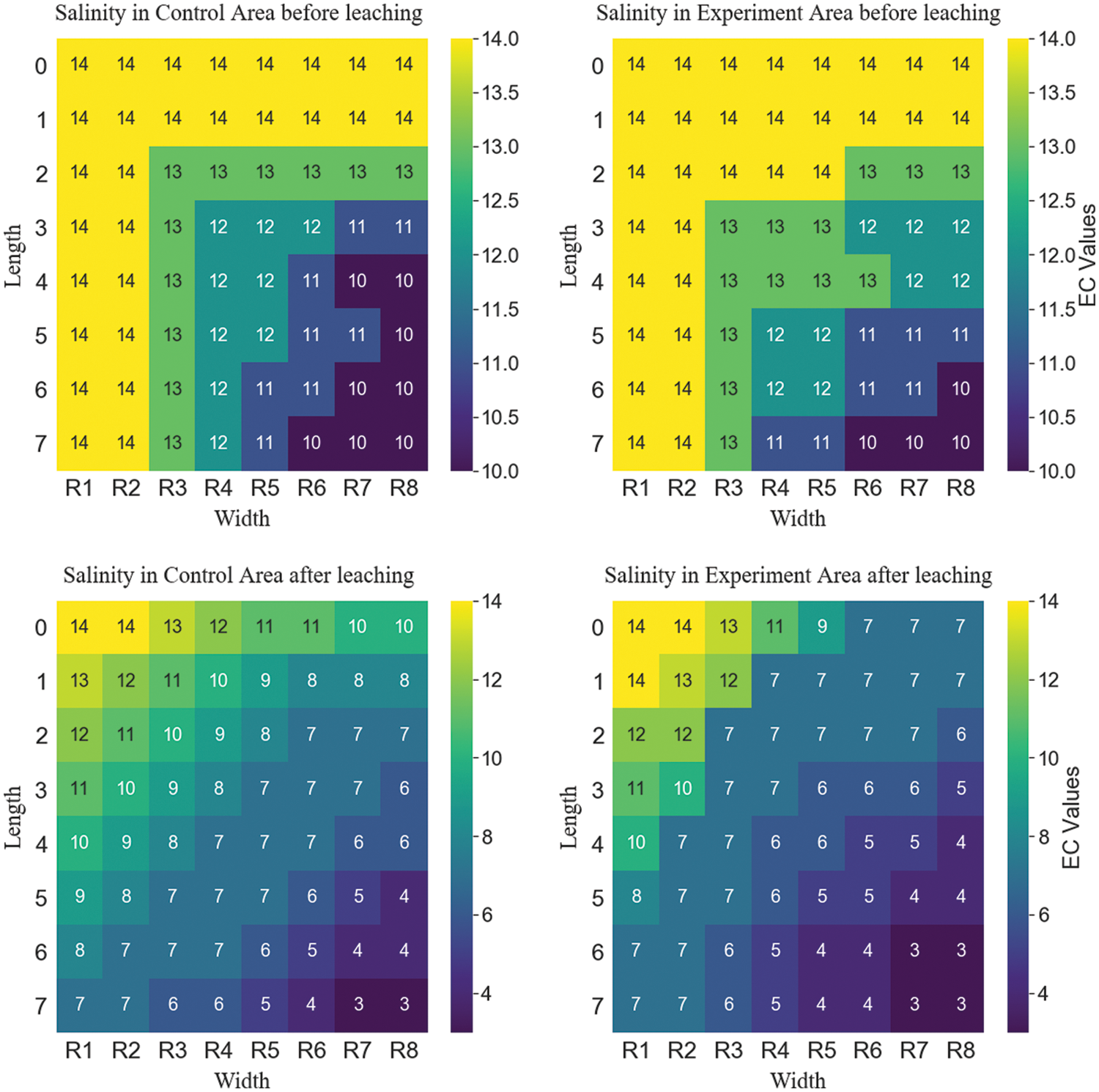
Figure 6: Salinity comparisons

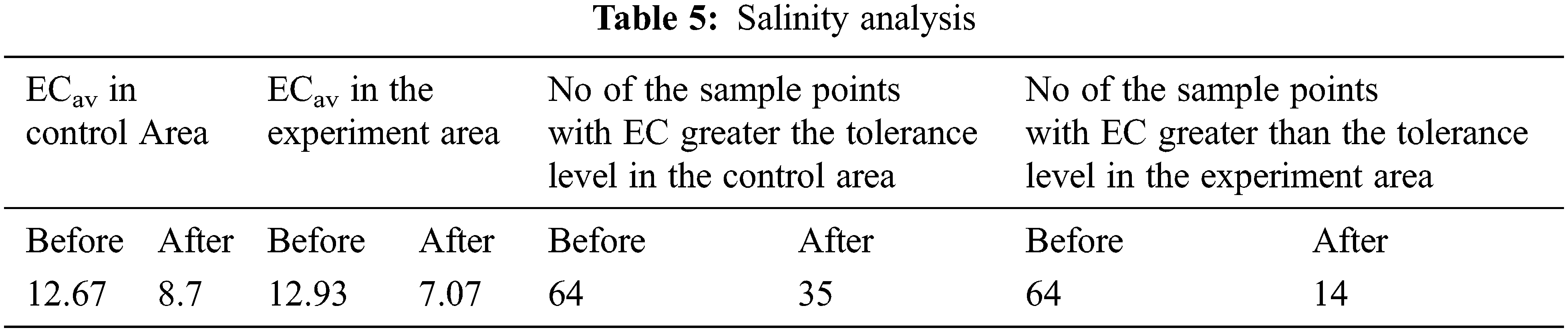
ECav in the control area is reduced from 12.78 to 8.7 dSm−1, after the application of leaching by the traditional method. In the experiment area, ECav is reduced from 12.93 to 7.07 dSm−1, with the application of smart LF of irrigation water. Smart leaching is more effective in the experiment area as compared to the traditional leaching process applied in the control area. The number of sample points with salinity level, more than the targeted level of soil salinity, was reduced from sixty-four (64) to thirty-five (35), in the control area, and from sixty-four (64) to fourteen (14) sample points in the experiment area. The smart LF application in the experiment area is more successful in reducing salinity as compared to the traditional method in the control area.

The performance of smart LF against the traditional methods in terms of average salinity, and the number of points above the target level reveals the success of smart LF of irrigation water against the traditional method. The smart LF of irrigation water is more effective in reducing the soil salinity as compared to the traditional leaching process. The proposed solution adjusts the irrigation water according to the prevailing temperature, humidity, and sunshine duration to recommend LF irrigation water that is more effective in reducing the soil salinity as compared to the traditional leaching process. Fig. 6 shows the distribution of the soil salinity in the experiment and control area before and after the application of the leaching process. From Fig. 6 it is observed that the proposed solution is more effective in reducing the soil salinity at more points as compared to the traditional leaching process.

5  Conclusion

Soil salinity is a soil degradation process that is a serious hazard to sustainable development in agriculture. Application of smart leaching by calibrated Evapotranspiration (ETc) is proposed for the Leaching Fraction (LF) of irrigation water to be more effective. Smart LF of irrigation water is proposed and implemented in a real-time environment. The ML model is proposed to adjust in Evapotranspiration rate according to humidity, sunshine, and wind speed to determine the ETc rate. The proposed ML model is accurate to predict the ETc to determine the smart LF of irrigation water. The LF of irrigation water is determined according to ETc, soil salinity level, irrigation water salinity level, and crop tolerance level. The field evaluation of the proposed solution of the smart LF reveals that the proposed solution is more effective in reducing the soil salinity in terms of average soil salinity and at a greater number of points. For future work, the proposed solution needs to be tested against different ML algorithms for a more accurate prediction of ETc. The proposed solution is based on the Blaney Criddle method of ETo rate determination. It needs to be tested against the Penman Montieth method and Pan Evaporation-based ETo determination.

Acknowledgement: The authors, therefore, gratefully acknowledge DSR technical and financial support.

Funding Statement: This project was funded by the Deanship of Scientific Research (DSR), King Abdul-Aziz University, Jeddah, Saudi Arabia under Grant No. (RG-11-611-43).

Conflicts of Interest: The authors declare that they have no conflicts of interest to report regarding the present study.

References

1. A. Singh, “Soil salinization and waterlogging: A threat to environment and agricultural sustainability,” Ecological Indicators, vol. 57, no. 1, pp. 128–130, 2015. [Google Scholar]
2. R. N. Bashir, I. S. Bajwa, M. Z. Abbas, A. Rehman, T. Saba et al., “Internet of things assisted soil salinity mapping at irrigation schema level,” Applied Water Science, vol. 12, no. 5, pp. 1–16, 2022. [Google Scholar]
3. R. N. Bashir, I. S. Bajwa and M. M. A. Shahid, “Internet of things and machine-learning-based leaching requirements estimation for saline soils,” IEEE Internet of Things Journal, vol. 7, no. 5, pp. 4464–4472, 2019. [Google Scholar]
4. Q. Liao, X. Li, F. Shi, Y. Deng, P. Wang et al., “Diurnal evapotranspiration and its controlling factors of alpine ecosystems during the growing season in northeast qinghai-tibet plateau,” Water (Switzerland), vol. 14, no. 5, pp. 1–15, 2022. [Google Scholar]
5. C. Lai, X. Chen, R. Zhong and Z. Wang, “Implication of climate variable selections on the uncertainty of reference crop evapotranspiration projections propagated from climate variables projections under climate change,” Agricultural Water Management, vol. 259, no. 1, pp. 107273, 2022. [Google Scholar]
6. J. Doorenbos and W. O. Pruitt, “Guidelines for predicting crop water requirements,” FAO Irrigation and Drainage Paper, vol. 24, no. 1, pp. 144–153, 1977. [Google Scholar]
7. T. Lemaitre-Basset, L. Oudin, G. Thirel and L. Collet, “Unraveling the contribution of potential evaporation formulation to uncertainty under climate change,” Hydrology and Earth System Sciences, vol. 26, no. 8, pp. 2147–2159, 2022. [Google Scholar]
8. T. Qian, A. Tsunekawa, F. Peng, T. Masunaga, T. Wang et al., “Derivation of salt content in salinized soil from hyperspectral reflectance data: A case study at minqin oasis, northwest China,” Journal of Arid Land, vol. 11, no. 1, pp. 111–122, 2019. [Google Scholar]
9. F. Wang, S. Yang, W. Yang, X. Yang and D. Jianli, “Comparison of machine learning algorithms for soil salinity predictions in three dryland oases located in Xinjiang uyghur autonomous region (XJUAR) of China,” European Journal of Remote Sensing, vol. 52, no. 1, pp. 256–276, 2019. [Google Scholar]
10. A. Singh, “Hydrological problems of water resources in irrigated agriculture: A management perspective,” Journal of Hydrology, vol. 541, no. 1, pp. 1430–1440, 2016. [Google Scholar]
11. M. Zaman, S. A. Shahid and L. Heng, “Guideline for salinity assessment, mitigation and adaptation using nuclear and related techniques,” in Springer Nature Switzerland AG, 1st ed, Cham, Switzerland, Springer Open, pp. 1–164, 2018. [Google Scholar]
12. M. C. Singh, J. P. Singh and K. G. Singh, “Development of a microclimate model for prediction of temperatures inside a naturally ventilated greenhouse under cucumber crop in soilless media,” Computers and Electronics in Agriculture, vol. 154, no. 1, pp. 227–238, 2018. [Google Scholar]
13. E. Asfaw, K. V. Suryabhagavan and M. Argaw, “Soil salinity modeling and mapping using remote sensing and GIS: The case of wonji sugar cane irrigation farm, Ethiopia,” Journal of the Saudi Society of Agricultural Sciences, vol. 17, no. 3, pp. 250–258, 2018. [Google Scholar]
14. D. K. Sharma and A. Singh, “Current trends and emerging challenges in sustainable management of salt-affected soils: A critical appraisal,” in Bioremediation of Salt Affected Soils: Indian Perspective, International Publishing, Cham: Springer, pp. 1–40, 2017. [Google Scholar]
15. H. N. Hellin, J. M. Rincon, R. D. Miguel, F. S. Valles and R. T. Sánchez, “A decision support system for managing irrigation in agriculture,” Computers and Electronics in Agriculture, vol. 124, no. 1, pp. 121–131, 2016. [Google Scholar]
16. B. M. Olivo, D. H. Rojas, J. M. Salinas and A. Pan, “Rules engine and complex event processor in the context of internet of things for precision agriculture,” Computers and Electronics in Agriculture, vol. 154, no. 1, pp. 347–360, 2018. [Google Scholar]
17. F. Rojo, E. Kizer, S. Upadhyaya, S. Ozmen, C. Ko-Madden et al., “A leaf monitoring system for continuous measurement of plant water status to assist in precision irrigation in grape and almond crops,” IFAC-PapersOnLine, vol. 49, no. 16, pp. 209–215, 2016. [Google Scholar]
18. S. M. A. El-Kader and B. M. M. El-Basioni, “Precision farming solution in Egypt using the wireless sensor network technology,” Egyptian Informatics Journal, vol. 14, no. 3, pp. 221–233, 2013. [Google Scholar]
19. R. Mulenga, J. Kalezhi, S. K. Musonda and S. Silavwe, “Applying internet of things in monitoring and control of an irrigation system for sustainable agriculture for small-scale farmers in rural communities,” in 2018 IEEE PES/IAS PowerAfrica, Cape Town, South Africa, pp. 841–845, 2018. [Google Scholar]
20. A. Haghverdi, B. G. Leib, R. A. W. Allen, P. D. Ayers and M. J. Buschermohle, “Perspectives on delineating management zones for variable rate irrigation,” Computers and Electronics in Agriculture, vol. 117, no. 1, pp. 154–167, 2015. [Google Scholar]
21. I. Mohanraj, K. Ashokumar, and J. Naren, “Field monitoring and automation using IoT in agriculture domain,” Procedia Computer Science, vol. 93, no. 1, pp. 931–939, 2016. [Google Scholar]
22. J. Gutierrez, J. F. V. Medina, A. N. Garibay and M. A. P. Gandara, “Automated irrigation system using a wireless sensor network and GPRS module,” IEEE Transactions on Instrumentation and Measurement, vol. 63, no. 1, pp. 166–176, 2014. [Google Scholar]
23. S. A. Nikolidakis, D. Kandris, D. D. Vergados and C. Douligeris, “Energy efficient automated control of irrigation in agriculture by using wireless sensor networks,” Computers and Electronics in Agriculture, vol. 113, no. 1, pp. 154–163, 2015. [Google Scholar]
24. N. Sales, O. Remedios and A. Arsenio, “Wireless sensor and actuator system for smart irrigation on the cloud,” in Proc. of IEEE World Forum on Internet of Things (WF-IoT), NW Washington DC, United States, pp. 693–698, 2015. [Google Scholar]
25. N. M. C. Garcia, A. G. B. Lozano and Y. A. R. Solis, “A crop planning and real-time irrigation method based on site-specific management zones and linear programming,” Computers and Electronics in Agriculture, vol. 107, no. 1, pp. 20–28, 2014. [Google Scholar]
26. Y. L. Xie, D. X. Xia, L. Ji and G. H. Huang, “An inexact stochastic-fuzzy optimization model for agricultural water allocation and land resources utilization management under considering effective rainfall,” Ecological Indicators, vol. 92, no. 1, pp. 301–311, 2017. [Google Scholar]
27. Y. Feng, Y. Peng, N. Cui, D. Gong and K. Zhang, “Modeling reference evapotranspiration using extreme learning machine and generalized regression neural network only with temperature data,” Computers and Electronics in Agriculture, vol. 136, no. 1, pp. 71–78, 2017. [Google Scholar]
28. M. Ilic, S. Jovic, P. Spalevic and I. Vujicic, “Water cycle estimation by neuro-fuzzy approach,” Computers and Electronics in Agriculture, vol. 135, no. 1, pp. 1–3, 2017. [Google Scholar]
29. R. W. Coates, M. J. Delwiche, A. Broad and M. Holler, “Wireless sensor network with irrigation valve control,” Computers and Electronics in Agriculture, vol. 96, no. 1, pp. 13–22, 2013. [Google Scholar]
30. M. Gocic, S. Motamedi, S. Shamshirband, D. Petkovic, S. Ch et al., “Soft computing approaches for forecasting reference evapotranspiration,” Computers and Electronics in Agriculture, vol. 113, no. 1, pp. 164–173, 2015. [Google Scholar]
31. C. Goumopoulos, B. O. Flynn and A. Kameas, “Automated zone-specific irrigation with wireless sensor/actuator network and adaptable decision support,” Computers and Electronics in Agriculture, vol. 105, no. 105, pp. 20–33, 2014. [Google Scholar]
32. Q. Kong, H. Chen, Y. L. Mo and G. Song, “Real-time monitoring of water content in sandy soil using shear mode piezoceramic transducers and active sensing-A feasibility study,” Sensors (Switzerland), vol. 17, no. 10, pp. 1–8, 2017. [Google Scholar]
33. F. Karim and F. Karim, “Monitoring system using web of things in precision agriculture,” Procedia Computer Science, vol. 110, no. 1, pp. 402–409, 2017. [Google Scholar]
34. V. Ramachandran, R. Ramalakshmi and S. Srinivasan, “An automated irrigation system for smart agriculture using the internet of things,” in 15th Int. Conf. on Control, Automation, Robotics and Vision (ICARCV), Singapore, Malaysia, pp. 210–215, 2018. [Google Scholar]
35. P. Afrasiabikia, A. P. Rizi and M. Javan, “Scenarios for improvement of water distribution in doroodzan irrigation network based on hydraulic simulation,” Computers and Electronics in Agriculture, vol. 135, no. 1, pp. 312–320, 2017. [Google Scholar]
36. X. Shi, X. An, Q. Zhao, H. Liu, L. Xia et al., “State-of-the-art internet of things in protected agriculture,” Sensors (Switzerland), vol. 19, no. 8, pp. 3–24, 2019. [Google Scholar]
37. N. Ahmed, D. De and I. Hussain, “Internet of things for smart precision agriculture and farming in rural areas,” IEEE Internet of Things Journal, vol. 5, no. 6, pp. 4890–4899, 2018. [Google Scholar]
38. T. Popovic, N. Latinovic, A. Pesic, Z. Zecevic, B. Krstajic et al., “Architecting an IoT-enabled platform for precision agriculture and ecological monitoring: A case study,” Computers and Electronics in Agriculture, vol. 140, no. 1, pp. 255–265, 2017. [Google Scholar]
39. J. M. Talavera, L. E. Tobon, J. A. Gomez, M. A. Culman, J. M. Aranda et al., “Review of IoT applications in agro-industrial and environmental fields,” Computers and Electronics in Agriculture, vol. 142, no. 118, pp. 283–297, 2017. [Google Scholar]
40. M. R. Naqvi, M. W. Iqbal, M. U. Ashraf, S. Ahmad, A. T. Soliman et al., “Ontology driven testing strategies for IoT applications,” Computers, Materials & Continua (CMC), vol. 70, no. 3, pp. 5855–5869, 2022. [Google Scholar]
41. K. Sakthivelu, D. Jalihal and G. A. Kumar, “Techno-commercial feasibility of soil moisture scanner for efficient irrigation scheduling,” IFAC-PapersOnLine, vol. 49, no. 16, pp. 199–204, 2016. [Google Scholar]
42. Y. Wang, Y. Zhang, X. Yu, G. Jia, Z. Liu et al., “Grassland soil moisture fluctuation and its relationship with evapotranspiration,” Ecological Indicators, vol. 131, no. 1, pp. 108196, 2021. [Google Scholar]
43. A. R. Niaghi, O. Hassanijalilian and J. Shiri, “Estimation of reference evapotranspiration using spatial and temporal machine learning approaches,” Hydrology, vol. 8, no. 1, pp. 1–25, 2021. [Google Scholar]
44. M. R. Naqvi, M. W. Iqbal, S. K. Shahzad, I. Tariq, M. Malik et al., “A concurrence study on interoperability issues in iot and decision making based model on data and services being used during inter-operability,” Lahore Garrison University Research Journal of Computer Science and Information Technology, vol. 4, no. 4, pp. 73–85, 2020. [Google Scholar]
45. A. Faramiñan, P. O. Rodriguez, F. Carmona, M. Holzman, R. Rivas et al., “Estimation of actual evapotranspiration in barley crop through a generalized linear model,” MethodsX, vol. 9, no. 1, pp. 101665, 2022. [Google Scholar]
46. A. F. López, D. M. Sánchez, G. G. Mateos, A. R. Canales, M. F. V. García et al., “A machine learning method to estimate reference evapotranspiration using soil moisture sensors,” Applied Sciences, vol. 10, no. 6, pp. 1912, 2020. [Google Scholar]
47. R. G. Allen, R. Dhungel, B. Dhungana, J. Huntington, A. Kilic et al., “Conditioning point and gridded weather data under aridity conditions for calculation of reference evapotranspiration,” Agricultural Water Management, vol. 245, no. 1, pp. 106531, 2021. [Google Scholar]
48. D. S. Martínez, F. Holwerda, T. R. Holmes, E. A. Yepez, C. R. Hain et al., “Evaluation of remote sensing-based evapotranspiration products at low-latitude eddy covariance sites,” Journal of Hydrology, vol. 610, no. 1, pp. 127786, 2022. [Google Scholar]
49. B. Petkovic, D. Petkovic, B. Kuzman, M. Milovancevic, K. Wakil et al., “Neuro-fuzzy estimation of reference crop evapotranspiration by neuro fuzzy logic based on weather conditions,” Computers and Electronics in Agriculture, vol. 173, no. 1, pp. 105358, 2020. [Google Scholar]
50. L. Wang, B. Wu, A. Elnashar, W. Zhu, N. Yan et al., “Incorporation of net radiation model considering complex terrain in evapotranspiration determination with sentinel-2 data,” Remote Sensing, vol. 14, no. 5, pp. 1191, 2022. [Google Scholar]
51. Z. Ma, B. Wu, N. Yan, W. Zhu and J. Xu, “Coupling water and carbon processes to estimate field-scale maize evapotranspiration with sentinel-2 data,” Agricultural and Forest Meteorology, vol. 306, no. 1, pp. 108421, 2021. [Google Scholar]
Cite This Article
Copyright © 2023 The Author(s). Published by Tech Science Press.
This work is licensed under a Creative Commons Attribution 4.0 International License , which permits unrestricted use, distribution, and reproduction in any medium, provided the original work is properly cited.
Downloads
Citation Tools