Cooperative Channel and Optimized Route Selection in Adhoc Network

1  Introduction

For security reasons, the mobile Adhoc network uses extremely sensitive routing and employs a variety of communication channels to reach its objective. When nodes in a far away area communicate data wirelessly, there is a possibility that the reliability of the other nodes in the transmission will be compromised. Occasionally, information is forwarded to a node; however, if the receiver is unreliable or the forwarding node channel is unable to send all of the information, the network transmission is rendered useless; this condition has the potential to result in significant packet loss and network delay. In this proposed CRCN paradigm, protocol approaches are used to address transmission issues and provide the necessary solution for safely reaching the target [1]. In this proposed CRCN architecture, we offer a network lifetime extension-aware cooperative channel access network that is utilized to adapt to performing a multi-unbiased object function, with the following inputs:

We have developed a multi-unbiased adaptive design that selects a confident forwarder from a source to send packets to a destination. The protocol used in this research improves the network life of nodes, energy management, node decoding performance, and finds responsive forwarders to transmit the packets [2]. The purpose of this research is to develop a dependable mobile Adhoc network. We offer an ideal method for nodes to choose the channel that uses the least energy to connect to a neighbor, and then select the channel based on the unusable condition directly, or jointly, thereby paving the way and transmitting information with a confident neighbor. We assume that nodes have asymmetric transmission due to node usage; the available transfer power at both the source and forwarder can be any value; it is determined by the node utilization from the start to the current state. Fig. 1 illustrates how the proposed architecture offers a powerful best confident forwarder selection technique for constructing a path from source to destination.

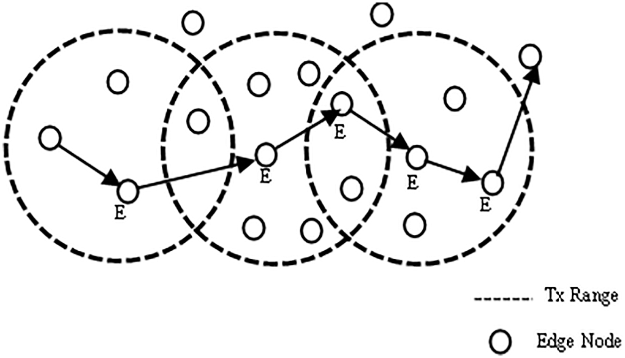
Figure 1: Transmission range nodes

Apart from the channel selection, this activity utilizes optimization calculations to provide multi-unbiased security and channel selection-based routing system. Here, we worked on the whale lioness calculations, which include lioness action into the whale to produce the ideal solution via perfect goal programming. The objectives identified in this suggested technique include numerous quality criteria derived from the media access control layer MAC, as well as distance and a confidence specification derived from the routing layer called the confidence of the node. We develop the fitness function to finalize the forwarder based on the afore said parameter adjustments [3]. The CRCN routing algorithm is composed of the following steps: (a) establishing quality measurements at two layers, (b) computing confidence levels, (c) identifying numerous disjoint paths, and (d) optimal pathfinding using the proposed multiple purpose channel selection methods. Thus, the proposed method provides an optimal transportation route with a favorable PDR, throughput, delay and energy consumption. The vital inputs of the suggested method for the confident based routing and lifetime extension aware channel access are as follows:

•   Designing a multi unbiassed optimization system for reliable routing by recognizing the above quality of service metrics and a confidence parameter as multi unbiassed.

•   Using many unbiassed models, i.e., energy, latency, link lifetime, distance, and confidence design, for the data transmission, so that the route is adopted and efficient, accelerating the convergence process [4], and reducing the number of discontinuous pathways.

It was necessary to extend the network’s life span to identify the best possible relay node for a given transmission power given at each source and relay node. Relay node selection in the MAC layer was also influenced by the transmission gain and residual energy.

In this work, we have taken place channel selection when the routing packets sent to find the path reach the MAC layer. The rest of this manuscript is discussed as follows. The part II represents the literature surveys in brief. In part III, the document pointed out the CRCN-cooperative channel selection and optimized route formation based on confidence in the Adhoc network is discussed. In section, IV informed the performance evaluation of the CRCN protocol and the end part carries out the CRCN conclusion, aims, and future opinions.

2  Literature Survey

Due to the restricted amount of power available for computing and radio transmission in ad hoc networks, node performance is critical. Additionally, there may be considerable constraints on the available bandwidth and radio frequencies [5]. Ad hoc networks can also be beneficial for law enforcement, emergency response and rescue missions. Because the ad hoc networks can be created rapidly and inexpensively, they are well suited for the commercial applications such as wireless networks or virtual classrooms [6]. It has been an extended time since these devices reached their full capability. Thanks to wireless technologies, these massive pieces of equipment may now communicate with any new machinery and be used anywhere. Wireless medical technology such as CodeBlue and MobiHealth [7] is in use. This model’s representation of the wireless channel includes broadcast omni-directional antennas, large-scale route loss, and fading. Utilize it in lieu of OSI layer design and specialized routing protocols to provide a comprehensive perspective of the routing challenge [8]. As the number of devices in an ad-hoc network grows, management becomes increasingly difficult. Connecting ad-hoc networks to wired networks is not possible. Ad-hoc networks provide a novel method of wireless communication for mobile hosts. There is no fixed infrastructure such as base stations in mobile switching [9]. We undertake energy-efficient routing before scheduling nodes’ transmissions to identify the least-powerful paths. The created schedule is based on end-to-end traffic data and preceding routing decisions [10]. A mobile node consumes battery power in addition to sending and receiving data by listening to the wireless medium for communication requests from other nodes [11]. The topology of the universe is constantly changing. The topology of a mobile ad hoc network is constantly changing as nodes move [12]. The radio range of the other nodes in the ad hoc network is continually changing, requiring constant updating of the routing information [13]. MANET’s have a wide range of applications, from large-scale moveable and dynamic networks to small networks constrained by their power supply. Along with the legacy applications that migrate from the old infrastructure environment, a considerable number of new services can and will be developed for the ad hoc context [14]. Each node within a network’s wireless range receives packets, regardless of whether they were meant for another node. Due to these characteristics, it is simple for each node to view the packets of other nodes or to the inject fault packets into the network. Vital nodes may experience battery drain and hence become unavailable for routing, resulting in broken links and a severe impact on the routing protocol’s performance [15]. Another key objective is to conserve energy on nodes to ensure the network’s longevity. Without an established communication infrastructure, a group of wireless mobile hosts forms its network dynamically. However, due to its open network architecture and shifting network topology, it is vulnerable to both internal and external attacks. Reactive routing protocols are more efficient in dynamic topologies such as MANET. A concerted effort is being made to improve (Ad-hoc On-Demand Distance Vector) AODV, the most widely used reactive routing technique. The Internet technical task committee has designated AODV as the official routing protocol for MANET [16]. Radios can broadcast over a large region. To determine whether a packet should be sent or received locally, each node within that range must receive it. Even if the majority of these packets are discarded, they use energy under this basic energy model [13]. The capacity of the power management system to respond to variations in traffic load is reflected in the length of the soft-state timer. We give methods for determining a neighbor’s power management [17], as broadcasting to a sleeping node is not the same as broadcasting to an active node. There are a variety of power control approaches that can be used to minimize network interference. Finally, the author Abdullah Waqas et al. [18] offered a routing algorithm for edge computing-enabled 5g networks, as well as a system of recommended metrics that is a function of the created and received interference in the network. The received interference term ensures that the Signal to Interference plus Noise Ratio (SINR) along the route remains greater than the threshold value, whilst the produced interference term ensures that only those nodes are chosen to forward packets that cause minimal interference to other nodes. The results indicate that the suggested method outperforms standard routing protocols in terms of network speed and outage probability.

3  CRCN Design and Implementation

3.1 Network Formation

Consider a Graph G=(N,E) which is created as a adhoc network with set of N, and E , where N=ni….nn stands for set of nodes, her i to n defines the number of nodes in the network. E is the set of neighbors of each node. We refer to this as E=ei….en , here ei is placed within the transmission variety of each node. The time taken to communicate between nodes can be calculated by the transmission delay between the two. Each node that transfer the data to it neighbor routing node and finally it reaches the destination, during which time it loses energy depending on the communication between the sender to neighbor. In this network, the distance between the nodes is calculated according to their location points and their displacement. The distance variations between the nodes vary continuously depending on the movements, at that point its location points will also change. These distance Dist variations are monitored from the beginning of the network, so that the distance changes are calculated as follows, where x1 x2 and y1 y2 denote its location points. The contact time between the two nodes is considered as their channel life CL .

Dist=|x1−x2|2+|y1−y2|2 (1)

3.2 Confidence Evaluation

The initial confidence values for each wireless node is calculated using a differential evolutionary method. After calculating the initial confidence values, the multi-objective method is used based on the Lion whale optimization LW , by which the functions of the nodes are accurately calculated. The degree of confidence for each node is designed using the degree of confidence calculated by one-hop contact of the nodes and the degree of confidence of the nodes in secondary contact. These two-degree vectors are connected using the weight factors for individual vectors. From the beginning of the network all normal nodes started to calculating the confidence level of the neighboring node.

3.3 One-Hop Trust Calculation

The degree of one-hop evolution is identified from a diverse evolution-based belief evaluation model as shown in Fig. 2. After calculating the one-hop confidence values, the table of confidence is broadcasting to one of its hop neighbors by the wireless sender.

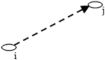
Figure 2: One hop communication

We calculate the one-hop confidence COH between the two nodes as shown below. Here SP is the sum of packets sent by a node, while RP is the sum of packets received by its neighbor ei from the sender Si . This information is obtained from the physical layer of the node, which i labelled in Eq. (2).

COH=RPSP (2)

Each node buys a one-hop report and checks the activities of its neighbors. When calculating the confidence value between two nodes, it falls between 0 and 1. Of these, 0 is taken as the confidence-less node and 1 is considered as a very reliable node. Each node start storing the information about the neighbor in an array format, they are:

•   Neighbor’s trust value,

•   The amount of energy present in the node

•   Changes in distances

•   Channel life between two nodes

•   Calculate how many routes can be set by a neighbor node

3.4 Secondary Node Trust Validation

Similarly, from the confidence tables obtained, the number of secondary hop confidence SHC values for each neighboring node is checked and then the average confidence value is determined by their counts.

SHC=1t∑COH

Here COH and SHC of each node take place at regular intervals t. In this way, the confidence degree CD is calculated with the help of weighted factors after checking the reports of one-hop and the confidence of the secondary nodes. In below Fig. 3 represent that the secondary hop communication, in this fugure there are three communication link as i,jandk.CD=COHα+COHβ

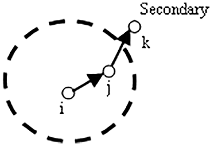
Figure 3: Secondary hop communication

With each iteration of the confidence IDC assessment, the degree of confidence is renewed in several stages based on varying average values.

IDC=ΔCDi+CD(1−Δ)

This variable average model uses weighted distribution based on the weighting factor. Where α and β are considered as the tunable weight value. These two together will be within the number 1.

4  Network Resource Validations

The energy parameter for each neighboring node is intended based on the number of packets transferred and the energy cost EC occurred because of receiving packets.

EC=ETP+ERP(Pi−1) , here, Pi indicates each bit of packet transmission ETP and ERP , explains the transmission packet counts and receiving packet counts of the network. The energy ratio ER is the ratio between the energy network cost and the initial energy Ei level of the nodes is computed as ECEi . The connection life of the current sender and the neighboring node is calculated using the moving speed MS of the current node and the neighboring node is calculated as Distt . As well as the moving directions varying depending on the moving angle of both the current node and the neighboring node, in this situation node speed variations, and angle deviations brings location coordinate variations, so the node position will continue to change till the end of network actions. From these values, the relative directional motion at both latitude and longitude is calculated as m and z .

m=cosθdiMSi−cosθdjMSj (3)

z=sinθdiMSi−sinθdjMSj (4)

The distance between both latitude and longitude is calculated in Eq. (5) and denoted as x and y.

x=x1i−x2j

y=y1i−y2j (5)

The transmission range of the node is signified by the radius r. Using these values as input, the connection lifetime for each node is calculated as seen below Eq. (6).

CL=−(mx+zy)+(m2+n2)r2−(my−zx)2m2+y2 (6)

Parameter distance is calculated by means of Euclidean distance estimation using latitude and longitude as inputs. The next parameter is to calculate how many routes are available for each node to reach the destination by its neighbor with node counts RC . The MRC parameter indicates the source path with the minimum distance that can be verified and destined through all available neighboring nodes.

4.1 Optimized Path Selection Initiation

Once the objective parameters for each node have been calculated, the LW optimization algorithm is invoked to calculate the optimal confidence values to finalize the path, in this optimization, approximate initial populations are generated for each entry in the confidence table. In the LW process, vector coefficients such as a and b are determined using equations

a=R1BVv−R1

b=vBV (7)

Here boundary value BV is taken as 2, v is the approximate generated vector, and R1 is a parameter that decreases in random number from 1 to 0.

4.2 The Following Steps are Implemented During Further Repetitions

The node status update during the optimization process is recognized by hunting behavior of LW , such as prey rounding, bubble-net attack, and prey search. Through the process of prey rounding, the distance vector DV is determined as ( bBAS−P ). P is the current population, and BAS is the best search agent status vector for the first iteration of the LW . At the stage of exploitation, the bubble-net attack process involves with the support of a spiral bubble-net attack, which uses the whale’s helix-shaped motion as follows to find the location of each population.

Pi+next=DVcos⁡(πIBV)+SPieIc (8)

Here c is a continual that describes the shape of a logarithmic loop, and I is the number designated from the interval from −1 to 1. SPi is a selected population in the present iteration taken as SPi=aDV−BAS .

Using the LW process, the vector vr is generated, which is approximately selected from the range between 0 to 1. The search space is improved by utilizing the LW update rule as follows Eqs. (9) and (10),

if(vr<0.5) (9)

SPi=aDV−BASelse

SPi+next=DVcos⁡(πIBV)+SPieIc (10)

Population-related solution vectors are calculated using the following Eq. (11),

SPi+next=1(0.05+1−0.1R1)(P(R10.05+1−0.1R1R2))+aDV(0.1R1−0.05) (11)

where R1 and R2 are approximate random numbers selected between 0 and 1. Later fitness F value is calculated by combining estimated parameters such as confidence IDC , energy EC , CL , distance DistC and route counts RC for each solution vector, which is labeled in Eq. (12).

F=15aDistRC+IDC+EC+CL+RCMRC (12)

If the developed solution has more F compared to the previous iteration, the solution will be sent to the next iteration, Otherwise the old re-solution is used to create the next random solution in further iterations. Once the maximum number o repetitions of the recalculation are reached when the required criteria are met based on the best global solution, the iterative process is stopped. The estimated optimal confidence value is used to select the best forwarding node to transmit the data packet and we can finalize the node is confident.

4.3 Multi-Purpose Optimization Evaluated in MAC Layer

Second multi-purpose optimization is used in the mac layer for optimal medium access-based transmission during data transmission. During the data transfer period, node sends request to send- RTS packet to a targeted node to book the channel. The required time node takes for the data transmission is enclosed along with the RTS packet is calculated as follows: Here TRTSD defines the total time required to forward the data from a node to the next confident neighbor.

TRTSD=ACKt+2SIFSt+8+CTS(BD+PS)BW (13)

Here BD meant the data bytes holding to transfer, PS describes the data packet size, BW explains the current bandwidth to transfer the packets, CTS defines the channel free status as clear to send packet send to the RTS sender, this packet transferred after the period of short inter frame space period SIFS multiplied with 2 to avoid the channel competition issues as shown in Figs. 4 and 5, ACK tells the acknowledgement of the data packet reception by the neighbor node. Later RTS sender waiting time SW is calculated as follows to get the CTS message: Here MBO defines the maximum back off period at mac layer.

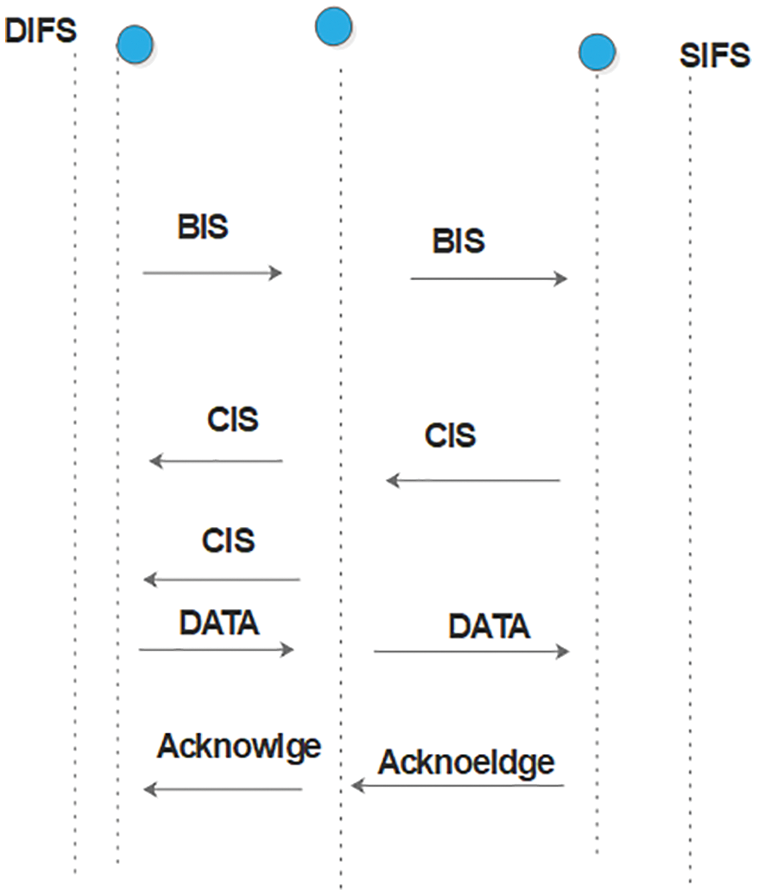
Figure 4: Channel selection

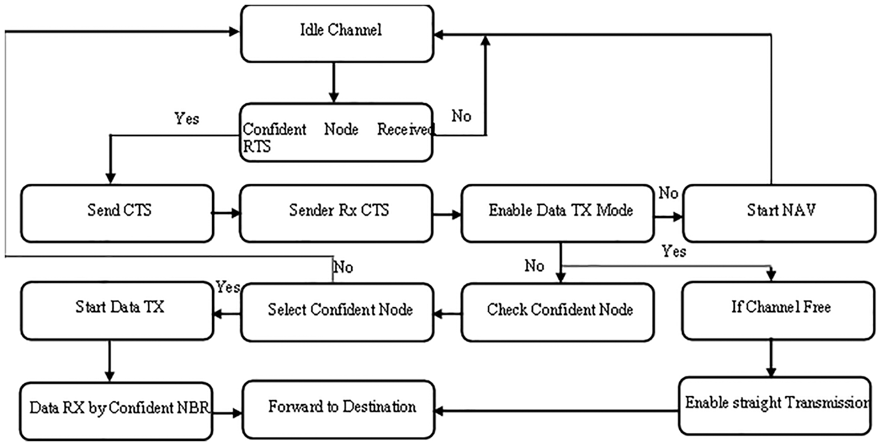
Figure 5: Communication at MAC layer

SW=Δ+SIFS+MBO+IN (14)

Even after the waiting period if the node is unable to get the channel confirmation, it cancels the previous request and initiates the new one as a timeout of CTS reception computed as CTSN=2Δ+CTS+SIFS+TRTS, where Δ is channel propagation delay. Once the channel is confirmed by the CTS reception then the sender transmits the packets, after the data transmission from the sender to the confident neighbor acknowledgment confirmation is computed by the node as

ACK=ACKt+2SIFSt+2Δ+(BD+PS)8BW (15)

In cooperative transmission period, the optimal TP at the source and forwarding node changes the approval time as follows Eqs. (16)–(18):

EACK=2−ACKΔ+2Δ+SIFS (16)

Then the confident node CSt not replied timeout is computed as

CSt=2Δ+CTS+RTS+SIFSP+IDCS (17)

and the confident node connection CSC duration is computed as

CSC=ACKt+2SIFSt+2(BD+PS)8BW (18)

Then, the waiting period for the CSw frame is determined

CSw=CSC+(BD+PS)8BW+ACKt+2SIFS+2Δ (19)

Then, the time takes for the data packets to reach the BS is calculated as DD=+SIFS+ACK

After receiving the RTS frame, the node that received the packet sends the CTS packet to the source node after the SIFS period. Here, direct transmission is used if the channel is free with no competition, and the ACK packet is sent to the source node when the data transfer is complete.

If another transaction occurs within that transmission region at the same time, the joint exchange is initiated by updating CCTS as follows Eq. (20)–(23),

CCTS=CIDC+CCTSW+SIFS (20)

CIDC=2Δ+MBO+CTS+SIFS+CT (21)

CT=8CPHBW//ConfidentNodeTime (22)

CCTSW=8+CTBD+PSBW+SIFS+2Δ (23)

If the frame transmission delay is less than the CTS duration, the transmission period will be renewed as DT=D+SIFS+Δ . Forwarder back off helpfulness calculated as per the node energy metric EM , direct and cooperative transfer rate as inputs. The energy parameter is computed as follows Eq. (24),

EM=REIE−STP (24)

Transmission power parameter is computed as ratio between the straight connection power STP=TP and cooperative forwarder channel power FPc computed as below Eqs. (25)–(28).

FPc=FP+STP (25)

φ=μ2log(λ2+TS+ρ) (26)

TS=D+SIFS+Δ (27)

FP=φ−(TR2RT2)(RG)2Dist−α (28)

Here μ , ρ and λ are the Lagrangian multipliers. Also, transmission rate parameter is computed as ratio between the STP rate and FPc rate. Where RT is the rate of transmission, TS is the packet delivery period, RG explains the receiving channel gain, This is where the cooperative transmission power is estimated as a sum of the optimal transmit power at source and the individual relaying nodes. The forwarder node power is computed as FP . Α defines the constant propagations as 2. From these values, the forwarder back off helpfulness FPH is computed as Eq. (29):

FPH=βFPcSTPEIRE−TPTRBW (29)

beta is set to ensure timely selection of the forwarder. Based on the estimated optimal transmission power, the forwarder power strong helping node for the current transmission is calculated as FPH . If the estimated FPH is less than the current FPH period, the newly rated FPH is assigned as the optimal departure period to achieve effective data transmission, which is designed in Eq. (30).

MaxFPH=min(maxFPH,MBO) (30)

5  Results and Discussions

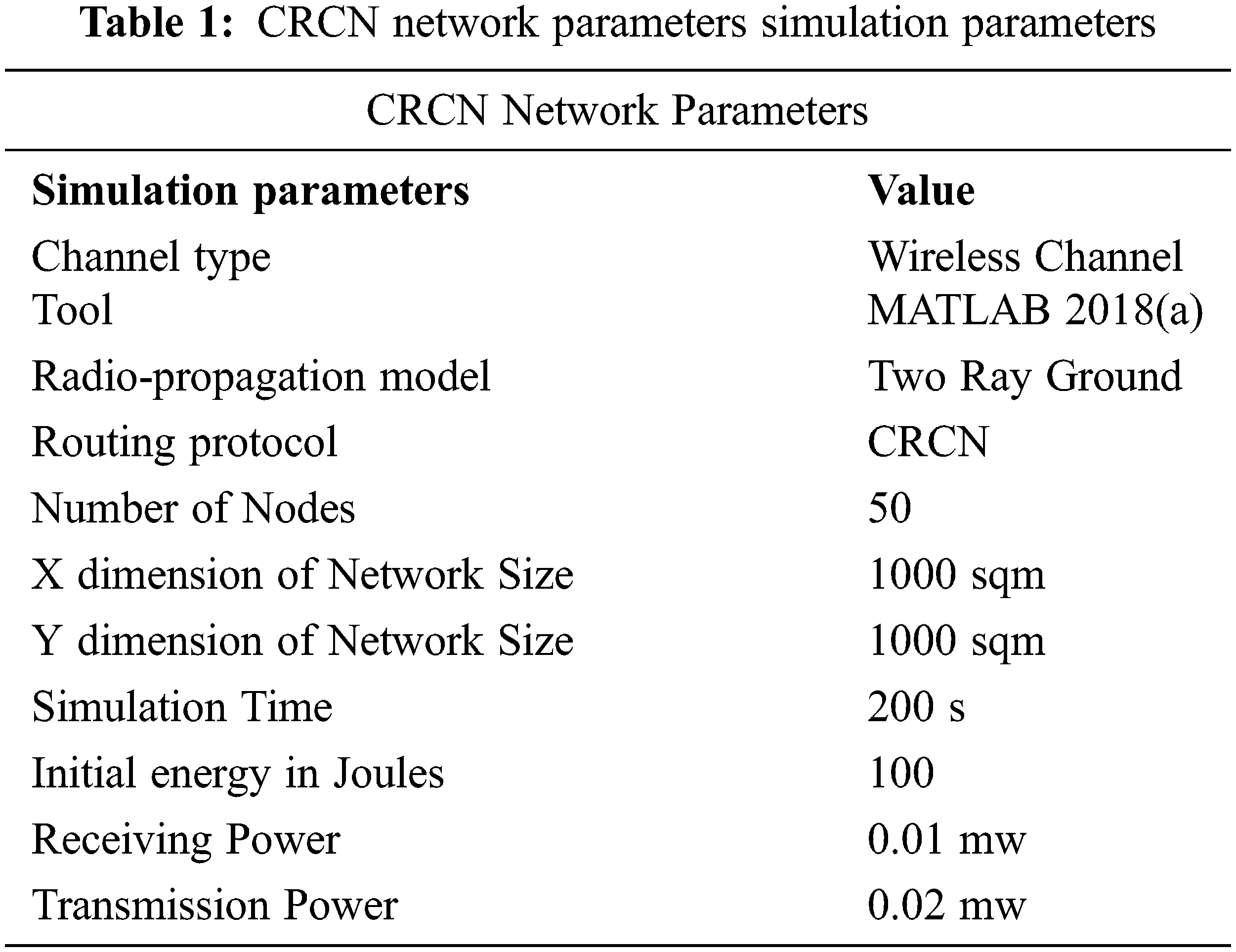
Network size is tested as 1000 × 1000 within an area in this experiment. As well as making changes to protocol routing and the mac layers and testing the performance of those changes in graphs format as given below Tab. 1. This protocol tells the best way to select a reliable forwarder and select the appropriate channel for the packets as they go through the network at regular intervals, here we see their test results.

Packet delivery ratio is the percentage of packets conventional at the destination depending on the number of packets shipped. Here, the CRCN protocol has received more packets at the destination. This Fig. 6 shows that this is achieved by the neighbor’s reliable selection module and by changing the channel selection method on the mac layer. By adding the largest number of packets to the destination, the designed CRCN protocol can see to it that the data packets are delivered to the destination in the correct manner. Here, we give the packet size as input and see the output of the resulting changes. By comparing between two techniques, the proposed method reaches the better Packet Size vs. Packet Delivery Ratio results.

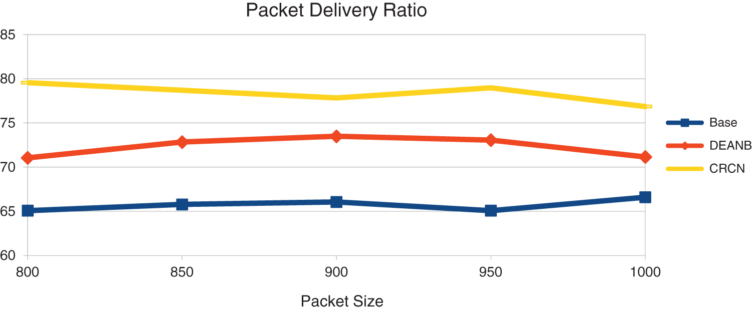
Figure 6: Packet size vs. packet delivery ratio

Throughput is the bits count of packets going to the destination. If the destination has received too many bits, we can know that the network is performing better. Here we can see that the CRCN protocol has received more packets than the compared others as shown in Fig. 7. This is an expression of the secured network and the network transmission is increased by selecting the proper node as the forwarder by the reports of the neighboring nodes and the reports of the nodes around it. And, by easily selecting the channel between them, more packet bits are delivered.

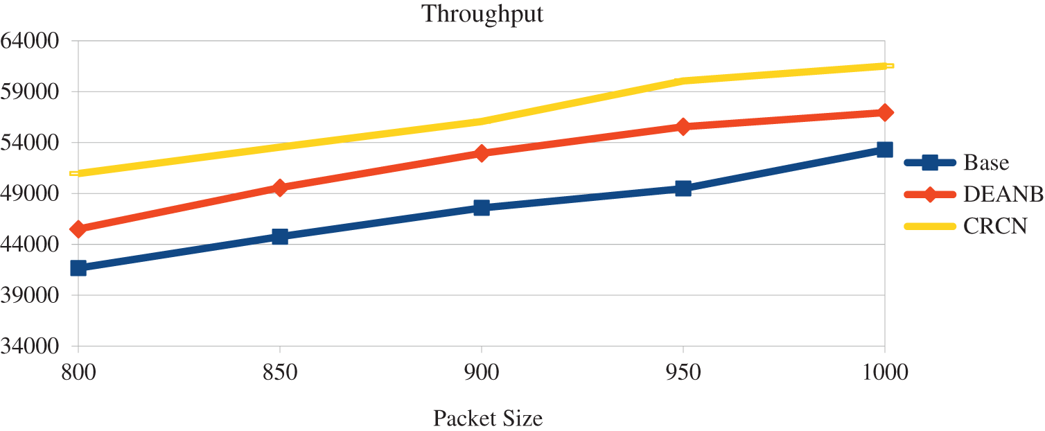
Figure 7: Packet size vs. throughput

This is an expression of the secured network, and the network transmission is increased by selecting the proper node as the forwarder by the reports of the neighbors and the reports of the second level nodes. And, by easily selecting the channel between them, more packet bits are delivered. Also, the reliability of the node is a factor, so in this proposed CRCN protocol, the reliability of the node and their channel selection act as an important parameter. By comparing between two techniques, the proposed method reaches the better packet transmission range vs. delay results. The Fig. 8 shows that its functions are very good.

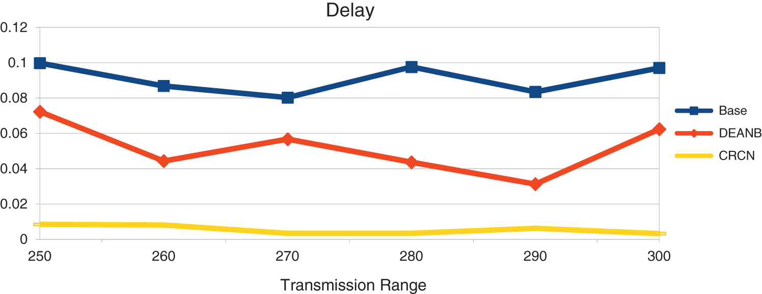
Figure 8: Transmission range vs. delay

Energy plays an important role in this. Network energy management is done with initial energy, remaining energy, packet transmission power, receiving power, so energy is also calculated as an important parameter when selecting the confident node. The Fig. 9 shows that the amount of energy stored in the network has increased due to this. Energy will be depleted very fast by unreliable nodes and that issue is solved here. Also, packets may expire if the correct channel is not set. The same issue is solved here. Due to this, the remaining energy in CRCN has increased.

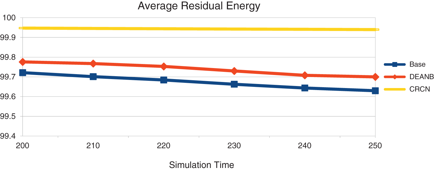
Figure 9: Simulation time vs. remaining energy

6  Conclusion

In this study, the steps show how the node acts as a confident forwarder and shares the channel in a way that is compatible with communication. We calculate the confidence of the node at the start of the network with the reliability report of the one hop and the reliability report of the secondary hop report. We figure out the combined confidence and use the same node as the most confident node as a forwarder, so we can move things along faster. When the routing packets sent to find the path reach the MAC layer, the next node in the path can be contacted directly if the channel is not used by any other nodes, and the channel is chosen. There will be no way to connect the channel unless there is a node that is sure. Then the path will be set. In this experiment, the amount of energy that is stored in the network is more than before. The nodes that aren’t reliable will use up a lot of energy very quickly, but that problem has been solved here. Even if the right channel is set, packets may not last long if they don’t reach the right person. The same thing has been solved here. Because of this, the amount of energy left in CRCN has gone up. When a node is confident, it chooses the best channel and the path is set up so that the network performance can be better than with the other protocols. To make the network work better, we can use this network security to let us use cognitive based channel selection and scheduling.

Funding Statement: The authors received no specific funding for this study.

Conflicts of Interest: The authors declare that they have no conflicts of interest to report regarding the present study.

References

1. R. H. Jhaveri Patel, N. M. Zhong and Y. Sangaiah, “Sensitivity analysis of an attack-pattern discovery based trusted routing scheme for mobile ad-hoc networks in industrial IoT,” IEEE Access, vol. 5, no. 6, pp. 20085–20103, 2018. [Google Scholar]
2. J. A. Anser, G. Han and H. Wang, “A novel reliable adaptive beacon time synchronization algorithm for large-scale vehicular ad hoc networks,IEEE,” Transactions on Vehicular Technology, vol. 8, no. 68, pp. 11565–11576, 2019. [Google Scholar]
3. C. F. Wang, Y. P. Chiou and G. H. Liaw, “Nexthop selection mechanism for nodes with heterogeneous transmission range in VANETs,” Computer Communications, vol. 1, no. 55, pp. 22–31, 2015. [Google Scholar]
4. W. Y. Lim, N. C. Luong, D. T. Hoang, Y. Jiao, Y. C. Liang et al., “Federated learning in mobile edge networks: A comprehensive survey,” IEEE Communications Surveys & Tutorials, vol. 8, no. 22, pp. 2031–2063, 2019. [Google Scholar]
5. Z. Lidong and Z. J. Haas, “Securing ad hoc networks,” IEEE Network, vol. 13, no. 6, pp. 24–30, 1999. [Google Scholar]
6. M. Haenggi, “Routing in ad hoc networks – a wireless perspective,” in First Int. Conf. on Broadband Networks, DC, USA, pp. 652–660, 2004. [Google Scholar]
7. V. Karpijoki, “Security in ad hoc networks,” in Proc. of the Helsinki University of Technology, Seminars on Network Security, Helsinki, Finland, pp. 1–14, 2000. [Google Scholar]
8. N. Krishnaraj and S. Sangeetha, “A study of data privacy in internet of things using privacy preserving techniques with its management,” International Journal of Engineering Trends and Technology, vol. 70, no. 2, pp. 43–52, 2022. [Google Scholar]
9. C. Yu, B. Lee and Y. H. Yong, “Energy efficient routing protocols for mobile ad hoc networks,” Wireless Communications and Mobile Computing, vol. 3, pp. 959–973, 2003. [Google Scholar]
10. S. Kulkarni, S. Ambaji and G. Raghavendra Rao, “A performance analysis of energy efficient routing in mobile ad hoc network,” International Journal of Simulations–Systems, Science and Technology–IJSSST, vol. 10, no. 1–A, pp. 1–9, 2010. [Google Scholar]
11. Y. Xu, H. Johnand and E. Deborah, “Geography-informed energy conservation for ad hoc routing,” in Proc. of the 7th Annual Int. Conf. on Mobile Computing and Networking, Rome, Italy, pp. 70–84, 2001. [Google Scholar]
12. A. Spyropoulos and C. S. Raghavendra, “Energy efficient communications in ad hoc networks using directional antennas,” in Proc. Twenty-First Annual Joint Conf. of the IEEE Computer and Communications Societies, BC, Canada, vol. 1, pp. 220–228, 2002. [Google Scholar]
13. M. V. S. S. Nagendranth, M. R. Khanna, N. Krishnaraj, M. Y. Sikkandar, M. A. Aboamer et al., “Type II fuzzy-based clustering with improved ant colony optimization-based routing (T2FCATR) protocol for secured data transmission in manet,” The Journal of Supercomputing, vol. First Online, pp. 1–22, 2022. [Google Scholar]
14. R. Zheng and R. Kravets, “On-demand power management for ad hoc networks,” in Proc. IEEE INFOCOM 2003. Twenty-second Annual Joint Conf. of the IEEE Computer and Communications Societies, BC, Canada, vol. 1, pp. 481–491, 2003. [Google Scholar]
15. T. Vaiyapuri, V. S. Parvathy, V. Manikandan, N. Krishnaraj, D. Gupta et al., “A novel hybrid optimization for cluster-based routing protocol in information-centric wireless sensor networks for IoT based mobile edge computing,” Wireless Personal Communications, vol. First Online, pp. 1–24, 2021. [Google Scholar]
16. G. Priyanka, V. Parmar and R. Rishi, “Manet: Vulnerabilities, challenges, attacks, application,” IJCEM International Journal of Computational Engineering & Management, vol. 11, no. 1, pp. 32–37, 2011. [Google Scholar]
17. P. Rajamohan and W. C. Kong, “Performance analysis and special security issues of secure routing protocols in ad-hoc networks,” International Journal of Scientific Engineering and Technology, vol. 3, no. 8, pp. 1094–1099, 2014. [Google Scholar]
18. A. Waqas, H. Mahmood and N. Saeed, “Interference aware cooperative routing for edge computing-enabled 5G networks,” IEEE Sensors Journal, vol. 12, no. 5, pp. 325–336, 2022. [Google Scholar]
Cite This Article
Copyright © 2023 The Author(s). Published by Tech Science Press.
This work is licensed under a Creative Commons Attribution 4.0 International License , which permits unrestricted use, distribution, and reproduction in any medium, provided the original work is properly cited.
Downloads
Citation Tools