Performance Analysis of a Chunk-Based Speech Emotion Recognition Model Using RNN

1  Introduction

Artificial intelligence speakers based on voice recognition are widely used for customer reception services. Robots and other devices assist humans in most industries and comprise simple voice recognition and display interfaces. Moreover, various studies are being conducted to improve the emotion recognition (ER) rate from voice signals to understand the exact intention of customers. ER technology analyzes the emotional states of humans by collecting and analyzing information from their voices or gestures. However, emotional states determined from voice signals are more accurate than those determined from gestures because expressing emotions with gestures may vary with culture. Recently, research on the analysis of emotions using various deep learning techniques, such as artificial neural network (ANN), convolutional neural network (CNN), and recurrent neural network (RNN), and studies on recognizing human emotions by extracting and analyzing the characteristics of voice signals in various manners have been conducted. ANN, CNN, and RNN have been employed in various fields, such as imaging [1–5], relation extraction [6], natural language processing [7], and speech emotion recognition (SER) [8].

SER using RNN-based long short-term memory (LSTM) and gated recurrent unit (GRU) has demonstrated improved performance in various studies because both techniques train on the audio signal considering the properties of the time-series sequence. However, the performance analysis of ER accuracy with respect to the simulation time has not yet been conducted. Therefore, in this study, we proposed a chunk-based SER (CSER) model that divides voice signals into 3-s long units to recognize the emotions from the individual chunks using LSTM, Bi-LSTM, GRU, and Bi-GRU techniques to analyze the performance of the SER accuracy with respect to the simulation time of the four RNN techniques.

The remainder of the study is organized as follows. Section 2 presents the related literature, and Section 3 describes the proposed CSER model. Section 4 presents the performance analysis of the SER accuracy and time efficiency of LSTM, Bi-LSTM, GRU, and Bi-GRU with the proposed CSER model. Finally, Section 5 presents the conclusions and further research directions.

2  Related Works

Many studies have been previously conducted to improve SER performance by combining the advantages of RNN and attention mechanisms (AM). AM is a technique based on the way humans focus on characteristic parts rather than using all information including the background when recognizing an object [9]. The initial AM was used to effectively analyze images by assigning weight to specific parts containing relatively important information in the field of neural network (NN)-based image processing. However, studies have been conducted to improve the performance of ER by applying the AM to the SER research fields to improve SER [10–20]. Tab. 1 lists the previous studies of SER using RNN with AM in terms of methods.

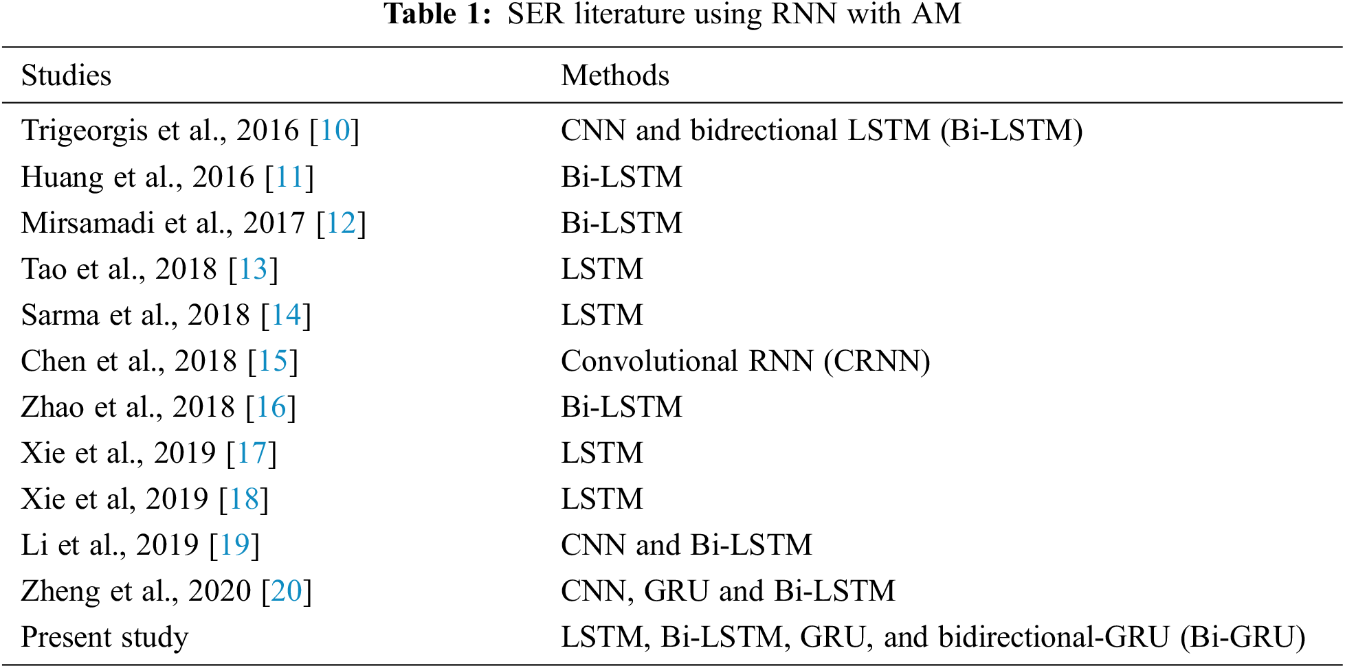
Studies listed in Tab. 1 analyzed emotions using the interactive emotional dyadic motion capture (IEMOCAP) dataset [21]. As shown in Tab. 1, SER studies using LSTM, Bi-LSTM, and GRU have been conducted [11–18]. Furthermore, the convergence studies of RNN and CNN were conducted to improve the SER accuracy [10,19,20]. However, studies on the performance analysis of the SER accuracy as a function of the simulation time of four RNN techniques, such as LSTM, Bi-LSTM, GRU, and Bi-GRU, have not yet been conducted.

3  Proposed CSER Model

In this section, we describe the overall structure of the proposed CSER model and LSTM, Bi-LSTM, GRU, and Bi-GRU techniques used to evaluate the performance, feature extraction, and AM of the proposed CSER model. The proposed CSER model divides the received voice signal into 3-s-long chunks and votes for recognized emotions using RNN techniques with hard and soft voting methods to eventually recognize voice emotion. Fig. 1 shows the flow chart of the proposed CSER model.

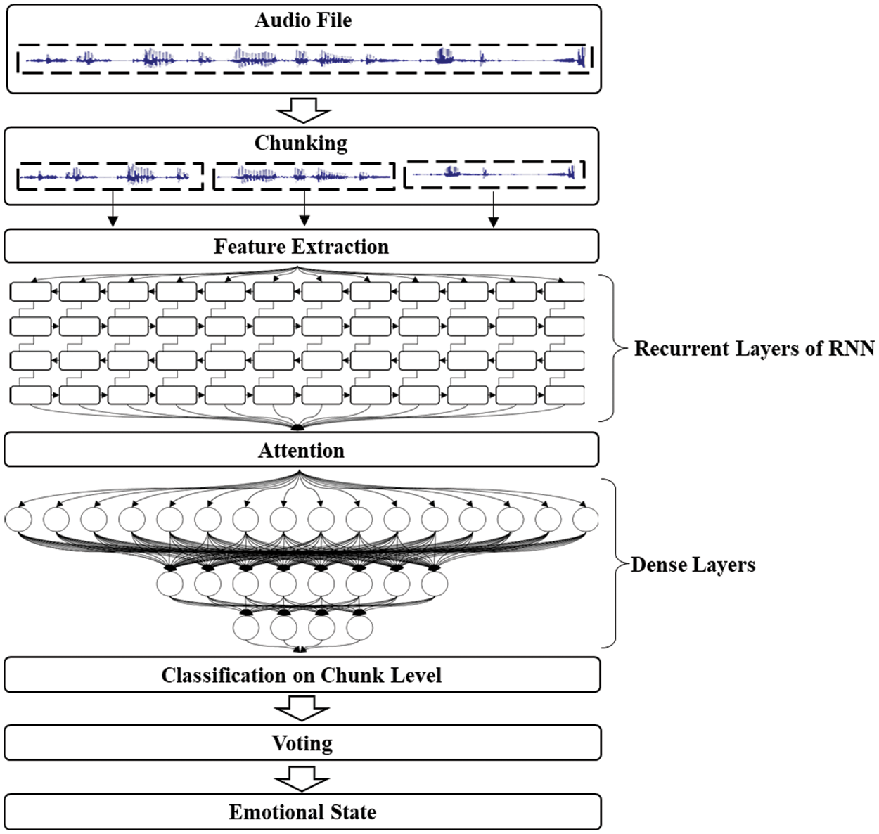
Figure 1: Flowchart of the proposed chunk-based SER (CSER) model

As shown in Fig. 1, feature extraction is performed in each chunk to evaluate the ER accuracy and simulation speed of the proposed CSER model. Four RNN techniques (LSTM, Bi-LSTM, GRU, and Bi-GRU) are used to recognize emotions from each of the chunked audio file. Subsequently, AM is used to calculate and reflect the importance of the voice signal according to the context of speech signals. Finally, the emotion recognized in each chunk is subjected to hard and soft voting to recognize the final emotion. The hard voting classifier in the proposed CSER model predicts the emotional state with the largest sum of votes from the chunks, whereas the soft voting classifier predicts the emotion with the largest summed probability of emotions from the chunks.

The detailed descriptions of the chunking process of audio signals, AM, LSTM, Bi-LSTM, GRU, and Bi-GRU techniques used in the proposed CSER model are presented in the following subsections.

3.1 Chunks of Audio Signals

In the proposed CSER model, an entire voice signal is divided into 3-s long intervals to accurately recognize emotions from all input audio signals. The minimum number of chunks of an entire voice signal can be expressed as

n=cl+1, (1)

where n is the number of chunks, c is the chunk size, and l is the audio length. After obtaining the number of chunks, the size h of the overlap can be calculated using Eq. (2) to ensure that the chunks overlap at regular intervals.

h=n×c−ln−1 (2)

After dividing the audio with different lengths into chunks of the same length, acoustic feature values are extracted from each chunk using the OpenSmile toolkit [22]. The feature extraction is described in the following section. Low-level descriptors (LLDs) are extracted from a 20–50-ms short frame to extract emotional features through RNN techniques from each chunk, and statistical functions are applied to the extracted LLDs to calculate high-level statistical functions, which are features of pronunciation units.

3.2 Feature Extraction

In the proposed CSER model, feature extraction is performed to extract and recognize voice features from each chunk. Zero-crossing rate (ZCR), root mean square (RMS), Mel vector, chroma, Mel-frequency cepstral coefficient (MFCC), and spectral features are extracted from each chunk for its ER.

ZCR calculates the sign change rate of the amplitude of each chunk. It refers to the rate at which the signal value passes through zero as the sign change rate, which is used as the most primitive pitch detection algorithm.

Z(i)=12N∑n=1N|(xi(n)−xi(n−1))| (3)

sgn(⋅) is the sign function given by

sgn(xi(n))={1(x≥0)−1(x<0), (4)

where x, N, and i are the amplitude, length, and index of the frame, respectively.

RMS is a value obtained by calculating the energy of each chunk frame (i.e., the sound intensity of each frame). It is the most basic measure of emotion, which is given by

RMS=∑i=1N⁡y(i)2N, (5)

where y(i) is the signal amplitude of the i-th chunk.

The Mel-scale spectrogram is a characteristic vector of the energy (dB) of each chunk according to time and frequency and is often used as a basic characteristic in ER. Chroma short-time Fourier transform is a feature vector representing the change of 12 distinctive pitch classes and can be characterized as a scale by extracting the energy of each scale from chunks according to time. MFCC is a feature that represents a unique characteristic of sound and can be extracted from an audio signal. The spectral feature is a statistical feature value in the frequency domain, and the frequency band spectrum is used as a statistical value for ER in addition to other features.

3.3 Recurrent Neural Network (RNN) Techniques

In this section, the LSTM, Bi-LSTM, GRU, and Bi-GRU techniques and self-AM for feature extraction used in the proposed CSER model are described.

3.3.1 Long Short-Term Memory (LSTM)

LSTM is a technique that supplements the shortcoming that, if learning continues for a long time in existing RNNs, initial learning is forgotten [23]. The values are adjusted by attaching cells called gates to the input, forget, and output layers of an RNN. The input gate decides whether to store new information, the forget gate decides whether to store previous state information, and the output gate controls the output value of an updated cell. Fig. 2 shows the structure of LSTM.

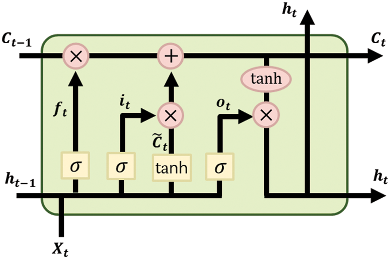
Figure 2: Structure of long short-term memory (LSTM)

In Fig. 2, xt and ht represent the input and hidden states at time t, respectively. Moreover, i, f, and o denote the input, forget, and output gates, respectively. First, LSTM uses a sigmoid function to determine the information to be eliminated. Then, it uses another sigmoid function and a tanh function to determine if new information should be stored in the cell state. The cell state is updated in the third step, and the output value is determined using the final sigmoid and tanh functions through which the output from the cell state is passed.

The LSTM used in this study consisted of continuously connected units in the left and right directions. At each step, the LSTM receives the hidden and cell states of the previous time step, receives the input value of the current step, performs computation through gates, updates the hidden and cell states, and transmits them to the next time step. Forget gate ft decides what information needs to be removed from the LSTM memory. The forget gate can be expressed as

ft=σ(Wf.[ht−1,xt]+bf), (6)

where W is the weight matrix, and b is the bias vector, which are used to connect the input layer, memory block, and output layer. The forget gate applies a sigmoid function on the previous hidden state ht−1 and current input value xt . An output value of zero indicates completely discarding the value, while a value of one represents the complete retainment of the value.

Input gate it decides whether or not the new information is to be added to the LSTM memory. This gate consists of sigmoid and tangent layers. The sigmoid layer determines which values need to be updated and the tanh layer creates a vector of new candidate values to be added to the cell state.

it=σ(Wf.[ht−1,xt]+bi), (7)

c~t=tanh⁡(WC.[ht−1,xt]+bc), (8)

where it decides whether the value should be updated, and c~t is the vector of new candidate values to be added to the cell state.

Subsequently, the previous cell state ct−1 is updated to the current cell state ct , which can be expressed as

ct=ft∗ct−1+it ∗ c~t, (9)

where ft is the result of the forget gate, a value between 0 and 1. Finally, the result is multiplied by the output of a sigmoid layer. Then, output gate ot is calculated using the output of sigmoid layer of ht−1 and xt .

ot=σ(Wo∗[ht−1,xt]+bo), (10)

ht=ot∗tanh⁡(ct), (11)

where ht is a value between −1 and 1. In this study, xt is the input chunked speech signal data. The input time-series speech signal data are expressed as X=[x1,x2,…,xN] , and the hidden state of memory cells is denoted by H=[h1,h2,…,hN], where N is the number of chunked speech data values.

3.3.2 Bidirectional-LSTM (Bi-LSTM)

Bi-LSTM is a modified LSTM [24] and comprises two independent hidden layers. It calculates the forward hidden sequence first followed by the reverse hidden sequence. Furthermore, it combines the two layers to obtain the output. Compared with LSTM, Bi-LSTM can improve the context available in the algorithm by effectively increasing the amount of information available in the network.

3.3.3 Gated Recurrent Unit (GRU)

GRU is an extended approach of LSTM [25] and is similar to LSTM with fewer parameters. The parameters are learned through the gating mechanism. Moreover, its internal structure is simpler, making it easier to train, because an update to its hidden state requires fewer computations. Moreover, it solves the vanishing gradient problem of LSTM. Fig. 3 illustrates the structure of GRU.

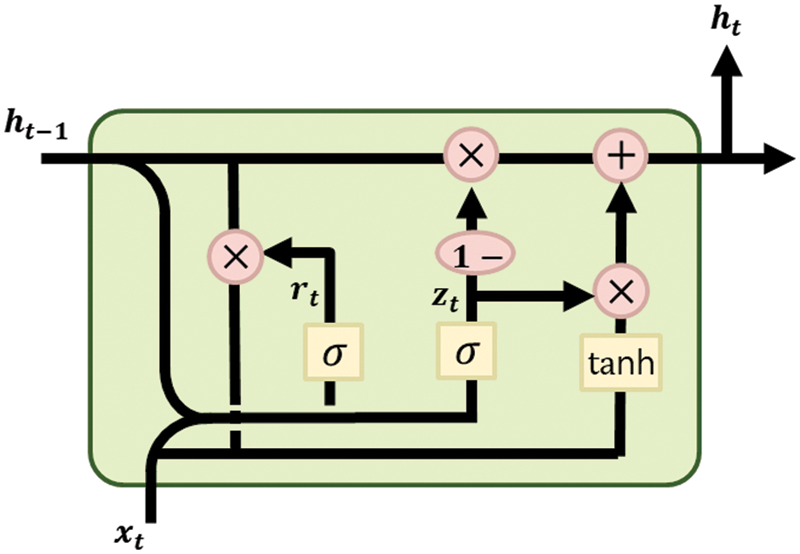
Figure 3: Structure of gated recurrent unit (GRU)

In LSTM, there are three gates—output, input, and forget—whereas there are only two gates—update and reset gates—in GRU. As shown in Fig. 3, the update gate, zt , determines which information can be retained to the next state and the reset gate, rt , determines how previous state information is combined with the new input information in GRU. The formula of GRU can be expressed as follows:

zt=σ(Wh.[ht−1,xt]), (12)

rt=σ(Wr.[ht−1,xt]), (13)

Candidate hidden state, ht , and current hidden state, ht , can be written as follows:

h~t=tanh(W.[rt∗ht−1,xt]), (14)

ht=(1−zt)∗ht−1+zt∗h~t (15)

where the definitions of σ , x, and h are the same as those in LSTM. ht and ht−1 denote the output of the current and previous states, respectively. xt denotes the speech data signal of the chunked voice signal. The input time-series chunked speech data are expressed as X=[x1,x2,…,xN] , and the hidden state of memory cells is denoted by H=[h1,h2,…,hN], where N is the number of chunked speech data values.

3.3.4 Bidirectional Gated Recurrent Unit (Bi-GRU)

Bi-GRU is an improved model that combines bidirectional RNN and GRU [24]. The structure of Bi-GRU is similar to that of Bi-LSTM, except for the cyclic unit. These two bidirectional networks can simultaneously use forward and reverse information. As GRU is simpler than LSTM, Bi-GRU is simpler than Bi-LSTM.

3.3.5 Attention Mechanisms (AM)

In this subsection, we describe the self-AM used in the proposed CSER model. AM was first proposed in the image processing field, and it aids a model to learn by focusing on specific function information. AM uses the state of the last hidden layer of LSTM or the implicit state of the LSTM’s output to fit the hidden state of the current moment input. However, in the field of SER, self-AM, which adaptively weights the current input voice signal, is more appropriate.

Sequential speech signals contain more emotional information than others such as signal interferences and noise. To focus on the emotional parts of a sequence, we learn the internal structure of the sequence with a focus on enhancing specific feature information in sentences using self-AM. Therefore, self-AM is an improved version of AM as it reduces dependence on external information and is better at capturing internal correlations of data or functions.

In the case of audio sequences that generally represent human emotions, adjacent frames exhibit similar acoustic characteristics. The query (Q), key (K), and value (V) of the i-th element for the voice data sequence X can be expressed as follows:

Qi=wqTxi, (16)

Vi=wvTxi, (17)

Ki=wkTxi, (18)

where xi is the i -th element of X. wq , wv , and wk are the linear projections that map the i -th element to the query, value, and key, respectively. The dimensions of Q, V, and K are 1×hp , where hp is a hyperparameter. Finally, the AM is computed using matrix multiplication on a set of sequences.

z=softmax(KTQdk)V, (19)

where Q, K, and V denote sets of queries, keys, and values, respectively, and dk is a scaling factor.

4  Simulation Results

4.1 Dataset

The dataset used in this study is the IEMOCAP database [21]. This database was comprised of five sessions, prepared using 10 actors who improvised or performed emotions based on a script in a mixed-gender pair, and analyzed by evaluators. Tab. 2 lists the IEMOCAP database.

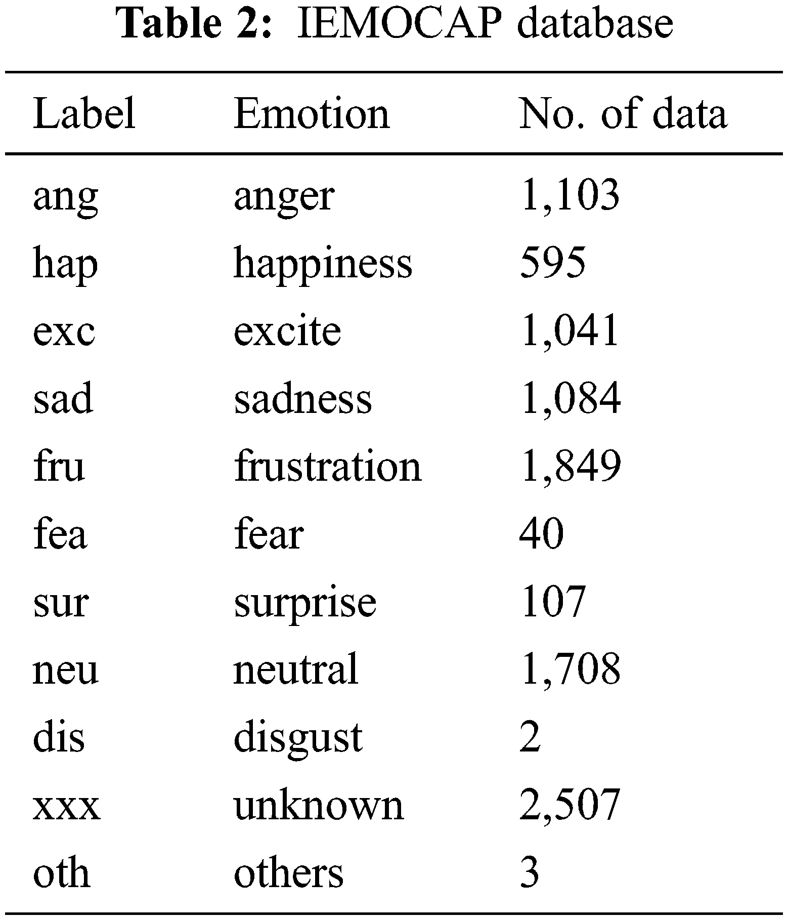
As shown in Tab. 2, the emotion data in this database comprise 10,039 voice files related to 11 types of emotions, such as anger, happiness, sadness, tranquility, excitement, fear, surprise, and disgust. Herein, the performance of the CSER model is analyzed using the emotion data of voice files related to anger, happiness, neutral, and sadness.

4.2 Performance Analysis of Hard Voting

In this section, we apply the LSTM, Bi-LSTM, GRU, and Bi-GRU techniques to the proposed CSER model and compare and analyze the accuracy and simulation time of the ER results through hard voting. Fig. 4 represents the confusion matrices of hard voting applied to the CSER model.

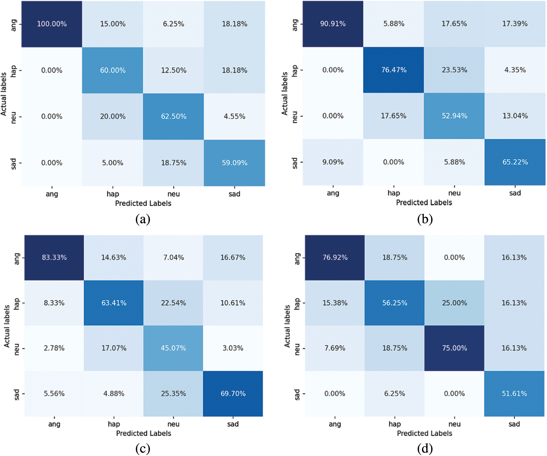
Figure 4: Confusion matrices of the proposed CSER model with hard voting: (a) LSTM, (b) Bi-LSTM, (c) GRU, and (d) Bi-GRU

Based on Fig. 4, four emotions are recognized from the voice signals with high probability when LSTM, Bi-LSTM, GRU, and Bi-GRU are applied to the proposed CSER. Furthermore, the prediction accuracy for distinct emotions such as anger is high. However, all four RNN techniques have the highest probability of diagonal matrices in confusion matrices for all emotions.

Figs. 5a and 5b show the accuracy and simulation time, respectively, for the four RNN techniques applied to the proposed CSER model. The final ER is evaluated using hard voting. Based on Fig. 6a, Bi-LSTM has the highest accuracy (63.97%), whereas LSTM has the lowest (60.05%). Tab. 3 summarizes the comparative performances of accuracy and simulation time of LSTM, Bi-LSTM, GRU, and Bi-GRU of the proposed CSER model when using hard voting.

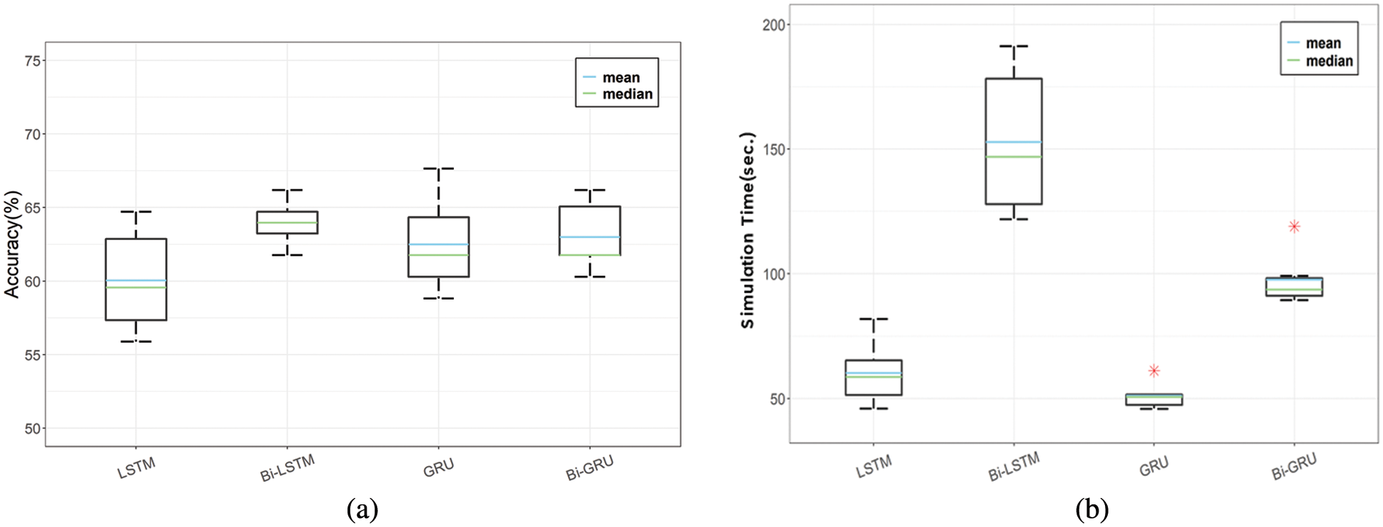
Figure 5: Performance comparison of LSTM, Bi-LSTM, GRU, and Bi-GRU of the proposed CSER model with hard voting: (a) accuracy and (b) simulation time

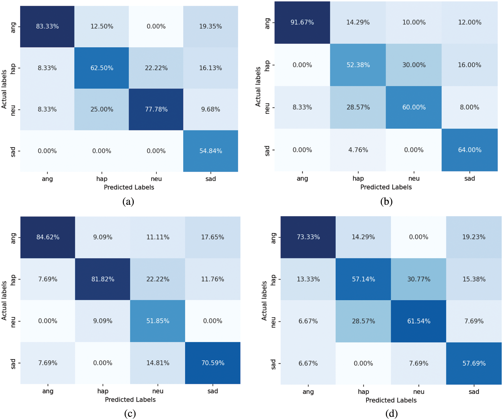
Figure 6: Confusion matrices of soft voting applied to the CSER model: (a) LSTM, (b) Bi-LSTM, (c) GRU, and (d) Bi-GRU

Tab. 3 shows the accuracy and simulation time when the final emotion is recognized using hard voting with the four RNN techniques applied to the proposed CSER model. Based on the Tab. 3, when applying the bidirectional technique for both the LSTM and GRU methods, the simulation time increased by approximately 2.5 and 1.8 times, respectively, and the accuracy increased by approximately 3.92% and 0.49%, respectively. In general, when evaluating emotions using hard voting, the time efficiency with respect to the simulation time is optimal for GRU since the structure of GRU is simpler than LSTM.

Furthermore, Tab. 3 shows that the simulation time of the GRU technique is the shortest when recognizing voice emotions using hard voting in the proposed CSER model. Tab. 4 lists the accuracy and time efficiency of GRU compared with the other three RNN techniques. The relative performance of accuracy and time efficiency compared to GRU when using hard voting is summarized in Tab. 4.

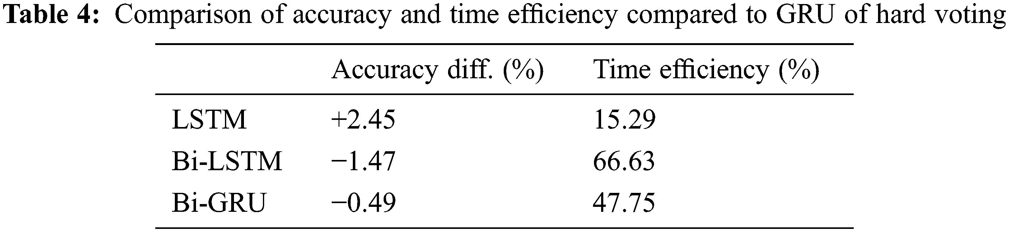
Tab. 4 lists the accuracy difference and time efficiency of three RNN techniques compared to GRU. The accuracy is increased by 2.45% compared to LSTM when speech emotion is recognized by GRU. However, compared to the Bi-LSTM and Bi-GRU, the speech recognition accuracy is decreased by −1.45% and −0.49%, respectively.

Nevertheless, as shown in Tab. 3, the simulation time is 51.02 s, which is the fastest among the four RNN techniques, when GRU is applied to the proposed CSER model. However, the time efficiency is increased by 15.29%, 66.63%, and 47.75% compared to the LSTM, Bi-LSTM, and Bi-GRU techniques, respectively, as shown in Tab. 4. Therefore, it can be confirmed that applying GRU to the proposed CSER model has the highest time efficiency relative to accuracy.

Therefore, we confirmed that applying GRU to the proposed CSER model resulted in the highest time efficiency with respect to the accuracy among the four RNN techniques.

4.3 Performance Analysis of Soft Voting

In this subsection, we apply the LSTM, Bi-LSTM, GRU, and Bi-GRU techniques to the proposed CSER model and compare and analyze the accuracy and simulation time of the ER results through soft voting. Fig. 6 shows the confusion matrices of emotion recognition results obtained by applying the four RNN techniques to the proposed CSER and using soft voting.

As shown in Fig. 6, the soft voting results recognize emotions from the voice signals with high probabilities, which are similar to the results of the hard voting in Section 4.2.

Figs. 7a and 7b show the accuracy and simulation time, respectively, for the four RNN techniques applied to the proposed CSER model, and the final ER is evaluated using soft voting. All four RNN techniques showed similar simulation accuracy. Both Bi-LSTM and Bi-GRU showed an increased simulation time of approximately 1.8 times compared with LSTM and GRU, respectively.

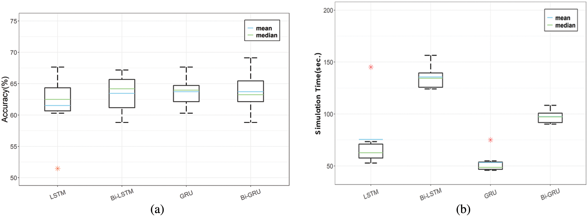
Figure 7: Performance comparison of LSTM, Bi-LSTM, GRU, and Bi-GRU of the proposed CSER model with soft voting: (a) Accuracy and (b) Simulation time

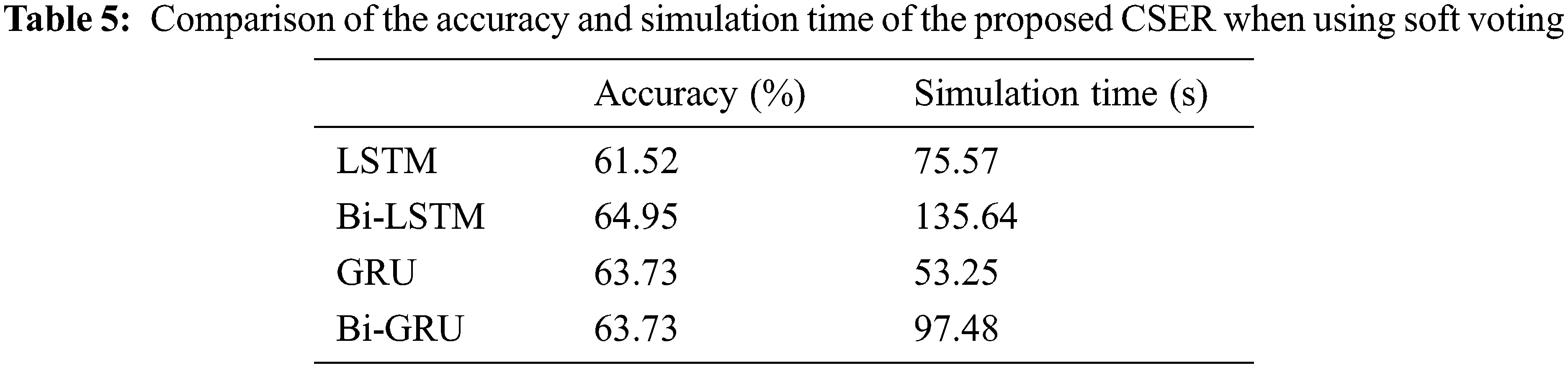
As shown in Tab. 5, when the bidirectional technique was applied to LSTM and GRU, the ER accuracy of LSTM increased by approximately 3.4%, but the accuracy of GRU did not increase. Therefore, GRU is the most efficient in terms of simulation time for the CSER model when using soft and hard voting. The relative performance of the accuracy and time efficiency compared to GRU when using soft voting is listed in Tab. 6.

Tab. 6 represents the results of the comparison of the accuracy and time efficiency between the GRU and the other three RNN techniques when recognizing emotions using soft voting in the proposed CSER model. When GRU is applied, the accuracy is increased by 2.21% compared to LSTM and decreased by 1.22% compared to Bi-LSTM, showing the same performance as that of Bi-GRU. However, when GRU is applied to the proposed CSER, the time efficiency of ER increased by 29.54%, 60.74%, and 45.37% compared to LSTM, Bi-LSTM, and Bi-GRU, respectively. Therefore, the GRU exhibits the highest performance in terms of simulation time for both hard and soft voting.

5  Conclusion

In this study, we proposed a CSER model in which a voice signal was divided into 3-s long chunks of voice signals to predict emotions using RNN techniques, recognize the emotions predicted in each chunk via hard and soft voting, and evaluate the performance. To evaluate the performance, the ER accuracy and simulation time of four RNN techniques (LSTM, Bi-LSTM, GRU, and Bi-GRU) were compared using hard and soft voting.

According to simulation results, GRU showed the best accuracy and time efficiency as a function of simulation time when emotion was recognized using LSTM, Bi-LSTM, GRU, and Bi-GRU techniques in the proposed CSER. It was confirmed that the time efficiency of GRU increased from a minimum of 15.29% to a maximum of 66.63% for hard voting and a minimum of 29.54% to a maximum of 60.74% for soft voting. Consequently, simulation results indicated that the GRU technique is the most efficient in terms of ER over simulation time using hard and soft voting. For further study, we plan to develop an ensemble CSER model that uses a combination of LSTM, Bi-LSTM, GRU, and Bi-GRU when recognizing emotions in each chunk of voice signals to increase the accuracy.

Funding Statement: This result was supported by the “Regional Innovation Strategy (RIS)” through the National Research Foundation of Korea (NRF) funded by the Ministry of Education (MOE) (2021RIS-004).

Conflicts of Interest: The authors declare that they have no conflicts of interest to report regarding the present study.

References

 1.  X. Zhao, W. Liu, W. Xing and X. Wei, “DA-Res2net: A novel densely connected residual attention network for image semantic segmentation,” KSII Transactions on Internet and Information Systems, vol. 14, no. 11, pp. 4426–4442, 2020. [Google Scholar]

 2.  Z. Huang, J. Li and Z. Hua, “Attention-based for multiscale fusion underwater image enhancement,” KSII Transactions on Internet and Information Systems, vol. 16, no. 2, pp. 544–564, 2022. [Google Scholar]

 3.  C. Dong, C. C. Loy, K. He and X. Tang, “Image super-resolution using deep convolutional networks,” IEEE Transactions on Pattern Analysis and Machine Intelligence, vol. 38, no. 2, pp. 295–307, 2015. [Google Scholar]

 4.  I. Hussain, J. Zeng Xinhong and S. Tan, “A survey on deep convolutional neural networks for image steganography and steganalysis,” KSII Transactions on Internet and Information Systems, vol. 14, no. 3, pp. 1228–1248, 2020. [Google Scholar]

 5.  B. Chen, J. Wang, Y. Chen, Z. Jin, H. J. Shim et al., “High-capacity robust image steganography via adversarial network,” KSII Transactions on Internet and Information Systems, vol. 14, no. 1, pp. 366–381, 2020. [Google Scholar]

 6.  H. Sun and R. Grishman, “Lexicalized dependency paths based supervised learning for relation extraction,” Computer Systems Science and Engineering, vol. 43, no. 3, pp. 861–870, 2022. [Google Scholar]

 7.  R. Mu and X. Zeng, “A review of deep learning research,” KSII Transactions on Internet and Information Systems, vol. 13, no. 4, pp. 1738–1764, 2019. [Google Scholar]

 8.  J. Lee and I. Tashev, “High-level feature representation using recurrent neural network for speech emotion recognition,” in Proc. Interspeech 2015, Dresden, Germany, pp. 1537–1540, 2015. [Google Scholar]

 9.  M. Luong, H. Pham and C. Manning, “Effective approaches to attention-based neural machine translation,” in Proc. 2015 EMNLP, Lisbon, Portugal, pp. 1412–1421, 2015. [Google Scholar]

10. G. Trigeorgis, F. Ringeval, R. Brueckner, E. Marchi, M. A. Nicolaou et al., “Adieu features? end-to-end speech emotion recognition using a deep convolutional recurrent network,” in Proc. 2016 IEEE ICASSP, Shanghai, China, pp. 5200–5204, 2016. [Google Scholar]

11. C. -W. Huang and S. S. Narayanan, “Attention assisted discovery of sub-utterance structure in speech emotion recognition,” in Proc. INTERSPEECH 2016, San Francisco, CA, USA, pp. 8–12, 2016. [Google Scholar]

12. S. Mirsamadi, E. Barsoum and C. Zhang, “Automatic speech emotion recognition using recurrent neural networks with local attention,” in Proc. 2017 IEEE ICASSP, New Orleans, LA, USA, pp. 2227–2231, 2017. [Google Scholar]

13. F. Tao and G. Liu, “Advanced LSTM: A study about better time dependency modeling in emotion recognition,” in Proc. 2018 IEEE ICASSP, Calgary, AB, Canada, pp. 2906–2910, 2018. [Google Scholar]

14. M. Sarma, P. Ghahremani, D. Povey, N. K. Goel, K. K. Sarma et al., “Emotion identification from raw speech signals using DNNs,” in Proc. Interspeech 2018, Hyderabad, India, pp. 3097–3101, 2018. [Google Scholar]

15. M. Chen, X. He, J. Yang and H. Zhang, “3-D convolutional recurrent neural networks with attention model for speech emotion recognition,” IEEE Signal Processing Letters, vol. 25, no. 10, pp. 1440–1444, 2018. [Google Scholar]

16. Z. Zhao, Y. Zheng, Z. Zhang, H. Wang, Y. Zhao et al., “Exploring spatio-temporal representations by integrating attention based bidirectional-LSTM-RNNs and FCNs for speech emotion recognition,” in Proc. Interspeech 2018, Hyderabad, India, pp. 272–276, 2018. [Google Scholar]

17. Y. Xie, R. Liang, Z. Liang, C. Huang, C. Zou et al., “Speech emotion classification using attention-based LSTM,” IEEE/ACM Transactions on Audio, Speech, and Language Processing, vol. 27, no. 11, pp. 1675–1685, 2019. [Google Scholar]

18. Y. Xie, R. Liang, Z. Liang and L. Zhao, “Attention-based dense LSTM for speech emotion recognition,” IEICE Transactions on Information and Systems, vol. 102, no. 7, pp. 1426–1429, 2019. [Google Scholar]

19. Y. Li, T. Zhao and T. Kawahara, “Improved end-to-end speech emotion recognition using self attention mechanism and multitask learning,” in Proc. INTERSPEECH 2019, Graz, Austria, pp. 2803–2807, 2019. [Google Scholar]

20. C. Zheng, C. Wang and N. Jia, “An ensemble model for multi-level speech emotion recognition,” Applied Sciences, vol. 10, no. 1, pp. 1–20, 2020. [Google Scholar]

21. C. Busso, M. Bulut, C. C. Lee, A. Kazemzadeh, E. Mower et al., “IEMOCAP: Interactive emotional dyadic motion capture database,” Language Resources and Evaluation, vol. 42, no. 4, pp. 335–359, 2008. [Google Scholar]

22. F. Eyben, M. Wöllmer and B. Schuller, “Opensmile: The Munich versatile and fast open-source audio feature extractor,” in Proc. 18th ACM Int. Conf. on Multimedia, New York, NY, USA, pp. 1459–1462, 2010. [Google Scholar]

23. S. Hochreiter and J. Schmidhuber, “Long short-term memory,” Neural Computation, vol. 9, no. 8, pp. 1735–1780, 1997. [Google Scholar]

24. M. Schuster and K. K. Paliwal, “Bidirectional recurrent neural networks,” IEEE Transaction on Signal Processing, vol. 45, no. 11, pp. 2673–2681, 1997. [Google Scholar]

25. J. Chung, Ç. Gülçehre, K. Cho and Y. Bengio, “Empirical evaluation of gated recurrent neural networks on sequence modeling,” in Proc. NIPS 2014 Workshop on Deep Learning, Montreal, QC, Canada, pp. 1–9, 2014. [Google Scholar]