A New Modified EWMA Control Chart for Monitoring Processes Involving Autocorrelated Data

1  Introduction

Quality control of products or services plays a very important role in the business and manufacturing industries. Statistical process control (SPC) is a powerful set of tools that are used to inspect, control, and improve the quality of processes [1], and control charts used for monitoring processes and detecting shifts in the process mean comprise a key tool for SPC. Shewhart [2] introduced the first control chart that is still widely used for monitoring and detecting large shifts in the process mean but is unsuitable for detecting small changes. Later, several researchers derived control charts for detecting small and large changes in process mean. The cumulative sum (CUSUM) control chart proposed by Page [3] is better than the Shewhart control chart for detecting small shifts in the process mean (see also [4,5]). Furthermore, Roberts [6] presented the exponentially weighted moving average (EWMA) control chart as another option for detecting small shifts in the process mean (see also [7,8]). Khan et al. [9] developed a new EWMA control chart statistic based on the modified EWMA statistic [10] that considers the past and current behavior of the process by introducing an extra constant in the modified EWMA statistic proposed in [9]. They compared its efficacy with the modified and standard control charts and found that the proposed control chart was more efficient in terms of the average run length (ARL) (a popular measure for control chart performance) and could detect shifts more quickly. Anwar et al. [11] proposed the modified mxEWMA control chart for a process in the presence of auxiliary information, while Aslam et al. [12] proposed the Bayesian-modified EWMA control chart for the process mean involving various loss functions.

The ARL is the average number of observations before a control chart signals that a process is out-of-control. There are two components: ARL0 and ARL1. ARL0 is the average number of observations for the process to remain in-control and should be as large as possible while ARL1 is the average number of observations until the process is signaled as out-of-control and should be as small as possible. Various methods to estimate the ARL have been reported, such as Monte Carlo simulation, Markov chain, Martingale, and numerical integration equations (NIEs) based on several quadrature rules (midpoint, trapezoidal, Simson’s rule, and Gauss-Legendre) [13]. Explicit formulas comprise a method for evaluating the ARL that requires solving integral equations. Crowder [7] used an integral equation approach to develop an approximation for the ARL of a Gaussian process on an EWMA control chart by using a Fredholm integral equation of the second kind. Champ et al. [14] also used this approach to evaluate the ARL on CUSUM and EWMA control charts and compared the results with those obtained by using the Markov chain approach. Moreover, the Fredholm integral equation of the second kind has been used to evaluate the ARL for many control charts [13]. Several researchers have focused on approximating the ARL to measure the efficacy of control charts by using many methods. Roberts [6] proposed using Monte Carlo simulation to estimate the ARL on the standard EWMA control chart. Harris et al. [15] studied serially correlated observations on a CUSUM control chart via Monte Carlo simulation. Vanbrackle et al. [16] investigated the NIE and Markov chain approaches to evaluate the ARL when the observations are from a first-order autoregressive (AR(1)) process with additional random error on EWMA and CUSUM control charts.

The modified EWMA statistic with an extra constant in the model that equally prioritizes historical and current information may degrade the performance of the control chart. Hence, we added one more constant to place more emphasis on current information over historical information. We hypothesized that the proposed control chart would provide very interesting properties (i.e., it would be more efficient at detecting small shifts in the process mean and would obtain the smallest ARL). Moreover, present a new modified EWMA control chart based on the modified EWMA statistic developed by Khan et al. [9] that prioritizes current information over historical information. In addition, we derive explicit formulas for the ARL for detecting changes in the process mean of a p-order autoregressive (AR(p)) process with exponential white noise running on the new modified EWMA control chart by using the Fredholm integral equation of the second kind and compared its efficiency with the ARL based on the well-know NIE method using the Gauss-Legendre rule.

2  The Properties of the Various EWMA Control Chart

The properties of the standard, modified, and new modified EWMA control charts are provided in the following subsections.

2.1 The Standard EWMA Control Chart

The standard EWMA control chart used for detecting small shifts in the process mean is defined as

Zt=(1−λ)Zt−1+λYt;t=1,2,3,…, (1)

where Zt is the EWMA statistic, Yt is the sequence of the AR(p) process with exponential white noise, and λ is an exponential smoothing parameter (0<λ≤1) .

The stopping time occurs when an out-of-control observation is firstly detected, which is sufficient to decide that the process is out-of-control. The stopping time τb for the standard EWMA control chart can be written as

τb=inf{t>0;Zt<aor Zt>b}, (2)

where a is a constant parameter known as the lower control limit (LCL) and b is a constant parameter known as the upper control limit (UCL). The upper side of the ARL for the AR(p) process on the standard EWMA control chart with an initial value (Z0=u) can be found. Now, function L(u) is defined as

L(u)=ARL=E∞(τb)≥T,Z0=u, (3)

where T is a fixed number (should be large) and E∞(.) is the expectation under the assumption that observations ϵt follow an F(yt,α) distribution.

The mean and the variance of the standard EWMA control chart can respectively be written as

E(Zt)=μ (4)

andVar(Zt)=(λ2−λ)σ2. (5)

For the control limit ( CL=μ0 ), the UCL and LCL of the standard EWMA control chart are respectively defined as follows:

LCL=μ0−L1σλ(2−λ) (6a)

andUCL=μ0+L1σλ(2−λ), (6b)

where μ0 is the target mean, σ is the process standard deviation, and L1 is an appropriate control width limit (L1>0) .

2.2 The Modified EWMA Control Chart

Khan et al. [9] developed a new EWMA control chart based upon the modified EWMA statistic of Patel et al. [10] that considers the past and current behavior of the process. This modified EWMA control chart is defined as

Mt=(1−λ)Mt−1+λYt+k(Yt−Yt−1);t=1,2,3,…, (7)

where Mt is the modified EWMA statistic, Yt is the sequence of the AR(p) process with exponential white noise, λ is an exponential smoothing parameter (0<λ≤1) , and k is a constant (k>0) . The stopping time τh for the modified EWMA control chart can be written as

τh=inf{t>0;Mt<g or Mt>h}, (8)

where g is the LCL and h is the UCL. The upper side of the ARL for the AR(p) process on the modified EWMA control chart with an initial value ( M0=u ) can be found. Now, we define function G(u) as

ARL=G(u)=E∞(τh)≥T,M0=u. (9)

The mean and the variance of the modified EWMA control chart are respectively defined as

E(Mt)=μ (10)

andVar(Mt)=(λ+2λk+2k2)σ2(2−λ). (11)

For the control limit ( CL=μ0 ), the UCL and LCL of the modified EWMA control chart can respectively be expressed as

LCL=μ0−L2σ(λ+2λk+2k2)(2−λ) (12a)

and UCL=μ0+L2σ(λ+2λk+2k2)(2−λ), (12b)

where L2 is an appropriate control width limit (L2>0) .

2.3 The Proposed New Modified EWMA Control Chart

The new modified EWMA control chart based on the modified EWMA control chart proposed by Khan et al. [9] is enhanced by adding one more constant to the model, which bestows more importance on current information than on historical information. The new modified EWMA control chart contains three constants: λ , k1 , and k2 in its derivation. Roberts [6] used k1=k2=0 in the original EWMA control chart whereas Khan et al. [9] suggested a modified EWMA control chart by assuming that k1=k2 , and similarly, Patel et al. [10] modified it by applying k1=k2=1 . The new modified EWMA control chart is derived as

Nt=(1−λ)Nt−1+λYt+k1Yt−k2Yt−1;t=1,2,3,…, (13)

where Nt is the new modified EWMA statistic, Yt is the sequence of the AR(p) process with exponential white noise, λ is an exponential smoothing parameter (0<λ≤1) , and k1 and k2 are constants (k1>k2>0) .

The stopping time τr for the modified EWMA control chart can be written as

τr=inf{t>0;Nt<l or Nt>r}, (14)

where l is the LCL and r is the UCL.

Now, the upper side of the ARL for the AR(p) process on the modified EWMA control chart with initial value N0=u can be found. First, we define function H(u) as

ARL=H(u)=E∞(τr)≥T,N0=u. (15)

The mean and the variance of the new modified EWMA control chart are respectively defined as

E(Nt)=(λ+k1−k2)μ0λ (16)

andVar(Nt)=[(λ+k1)2+k22−2λk2+2λ2k2−2k1k2+2λk1k2λ(2−λ)]σ2. (17)

Meanwhile, for control limit CL=(λ+k1−k2)μ0λ , the UCL and LCL of the modified EWMA control chart can respectively be expressed as

LCL=(λ+k1−k2)μ0λ−L3σ(λ+k1)2+k22−2λk2+2λ2k2−2k1k2+2λk1k2λ(2−λ) (18a)

and UCL=(λ+k1−k2)μ0λ+L3σ(λ+k1)2+k22−2λk2+2λ2k2−2k1k2+2λk1k2λ(2−λ), (18b)

where L3 is an appropriate control width limit (L3>0) .

3  Explicit Formulas for the ARL of an AR(p) Process on the New Modified EWMA Control Chart

The AR(p) process is defined as

Yt=δ+ϕ1Yt−1+ϕ2Yt−2+…+ϕpYt−p+ϵt;t=1,2,3,…, (19)

where δ is a constant (δ≥0) , ϕi is an autoregressive coefficient for i=1,2,…,p(|ϕp|<1) , and ϵt is an independent and identically distributed (iid) sequence ( ϵt∼Exp(α) ). The initial value for the AR(p) process mean is Yt−1,Yt−2,…,Yt−p=1 .

3.1 The Explicit Formulas

Explicit formulas for the ARL of the new modified EWMA control chart for an AR(p) process are derived as follows:

Nt=(1−λ)Zt−1+(λ+k1)δ+(λ+k1)ϕ1Yt−1+…+(λ+k1)ϕpYt−p+(λ+k1)ϵt−k2Yt−1.

If Y1 signals the out-of-control state for N1 , N0=u , then

N1=(1−λ)u+(λ+k1)δ+(λ+k1)ϕ1Yt−1+…+(λ+k1)ϕpYt−p+(λ+k1)ϵ1−k2v

If ϵ1 is the in-control limit for N1 , then l≤N1≤r . Consider function H(u)

H(u)=1+∫H(N1)f(ϵ1)d(ϵ1). (20)

Eq. (20) is a Fredholm integral equation of the second kind [17], and thus H(u) can be rewritten as

H(u)=1+∫lrL{(1−λ)u+(λ+k1)δ+(λ+k1)ϕ1Yt−1+…+(λ+k1)ϕpYt−p−k2Yt−1+(λ+k)y}f(y)dy.

Let w=(1−λ)u+(λ+k1)δ+(λ+k1)ϕ1Yt−1+…+(λ+k1)ϕpYt−p−k2Yt−1+(λ+k)y.

By changing the integral variable, we obtain the following integral equation:

H(u)=1+1λ+k1∫lrH(w)f{w−(1−λ)u(λ+k1)+k2Yt−1(λ+k1)−δ−ϕ1Yt−1−…−ϕpYt−p}dw. (21)

If Yt∼Exp(α) the f(y)=1αe−yα ; y≥0 , then

H(u)=1+1λ+k1∫lrH(w)1αe−1α{w−(1−λ)u(λ+k1)+k2Yt−1(λ+k1)−δ−ϕ1Yt−1−…−ϕpYt−p}dw. (22)

Let function C(u)=e(1−λ)uα(λ+k1)−k2Y−1α(λ+k1)+δα+ϕ1Yt−1+…+ϕpYt−pα , then we have

H(u)=1+C(u)α(λ+k1)∫lrH(w)e−wα(λ+k1)dw; l≤u≤r.

Let B=∫lrH(w)e−wα(λ+k1)dw , then H(u)=1+C(u)α(λ+k1)⋅B . Consequently, we obtain

H(u)=1+1α(λ+k1)e(1−λ)uα(λ+k1)−k2Yt−1α(λ+k1)+δα+ϕ1Yt−1+…+ϕpYt−pα⋅B. (23)

By solving for constant B, we obtain

B=∫lrH(w)e−wα(λ+k1)dw=−α(λ+k1)(e−rα(λ+k1)−e−lα(λ+k1))1+e−k2Yt−1α(λ+k1)+δα+ϕ1Yt−1+…+ϕpYt−pαλ(e−λrα(λ+k1)−e−λlα(λ+k1)).

By substituting constant B into Eq. (23), we arrive at

H(u)=1+e(1−λ)uα(λ+k1)−k2Yt−1α(λ+k1)+δα+ϕ1Yt−1+…+ϕpYt−pαα(λ+k1)(−α(λ+k1)[e−rα(λ+k1)−e−lα(λ+k1)]1+e−k2Yt−1α(λ+k1)+δα+ϕ1Yt−1+…+ϕpYt−pαλ[e−λrα(λ+k1)−e−λlα(λ+k1)]). (24)

Therefore, the explicit two-sided formulas for the ARL of an AR(p) process running on the new modified EWMA control chart by using the Fredholm integral equation of the second kind can be defined as

ARL2−sided=1−λe(1−λ)uα(λ+k1)[e−rα(λ+k1)−e−lα(λ+k1)]λek2Yt−1α(λ+k1)−δα−ϕ1Yt−1−…−ϕpYt−pα+e−λrα(λ+k1)−e−λlα(λ+k1). (25)

when l=0 , the explicit one-sided formulas for the ARL on the new modified EWMA control chart can be written as follows:

ARL1−sided=1−λe(1−λ)uα(λ+k1)[e−rα(λ+k1)−1]λek2Yt−1α(λ+k1)−δα−ϕ1Yt−1−…−ϕpYt−pα+e−λrα(λ+k1)−1 (26)

3.2 The Existence and Uniqueness of Explicit Formulas

Here, we show the existence and uniqueness of the solution to the integral equation in Eq. (22). First, we define

T(H(u))=1+1λ+k1∫lrH(w)1αe−1α{w−(1−λ)u(λ+k1)+k2Yt−1(λ+k1)−δ−ϕ1Yt−1−…−ϕpYt−p}dw (27)

Theorem 1. (Banach’s fixed-point theorem [18])

Let C[l,r] be a set of all of the continuous functions on complete metric (X,d), and assume that T:X→X is a contraction mapping with contraction constant 0≤s<1 ; i.e., ‖T(H1)−T(H2)‖≤s‖H1−H2‖∀H1,H2∈X . Subsequently, H(.)∈X is unique at T(H(u))=H(u) ; i.e., it has a unique fixed point in X.

Proof: To show that T defined in Eq. (27) is a contraction mapping for H1,H2∈C[l,r] , we use the inequality ‖T(H1)−T(H2)‖≤s‖H1−H2‖∀H1,H2∈C(l,r) with 0≤s<1 . Consider Eqs. (22) and (27), then

‖T(H1)−T(H2)‖∞=supu∈[l,r]⁡|C(u)α(λ+k1)∫lr(H1(w)−H2(w))e−wα(λ+k1)dw|

≤supu∈[l,r]⁡|‖H1−H2‖∞C(u)(e−lα(λ+k1)−e−rα(λ+k1))|

=‖L1−L2‖∞|e−lα(λ+k1)−e−rα(λ+k1)|supu∈[l,r]⁡|C(u)|

≤s‖L1−L2‖∞,

where s=|e−lα(λ+k1)−e−rα(λ+k1)|supu∈[l,r]⁡|C(u)| and C(u)=e(1−λ)uα(λ+k1)−k2Yt−1α(λ+k1)+δα+ϕ1Yt−1+…+ϕpYt−pα ; 0≤s<1 .

Therefore, as confirmed by applying Banach’s fixed-point theorem, the solution exists and is unique.

4  The NIE for the ARL of an AR(p) Process on the New Modified EWMA Control Chart

The NIE approach is widely used for evaluating the ARL. It can be based on several quadrature rules (midpoint, trapezoidal, Simson’s rule, and Gauss-Legendre), all of which give ARLs that are very close to each other [19]. When considering the problem of integrating function f(w) over [l, r], the interval of integration [l, r] is finite when using the midpoint, trapezoidal, and Simpson’s rules whereas it is infinite for the Gauss-Legendre rule [13]. Therefore, in this study, we used the Gauss-Legendre rule to evaluate the ARL. An integral equation of the second kind for the ARL on the new modified EWMA control chart for the AR(p) process in Eq. (24) can be approximated by using the quadrature formula. The Gauss-Legendre quadrature rule is applied as follows:

Givenf(aj)=f{aj−(1−λ)ai(λ+k1)+k2Yt−1(λ+k1)−δ−ϕ1Yt−1−…−ϕpYt−p}. (28)

The approximation for the integral is in the form

∫lrH(w)f(w)dw≈∑j=1mwjf(aj), (29)

where aj=r−lm(j−12)+l and wj=r−lm;j=1,2,…,m

Using the Gauss-Legendre quadrature formula, numerical approximation H~(u) for the integral equation can be found as the solution for the following linear equations:

H~(u)=1+1λ+k1∑j=1mwjH~(aj)f{aj−(1−λ)u(λ+k1)+k2Yt−1(λ+k1)−δ−ϕ1Yt−1−…−ϕpYt−p}. (30)

5  Comparison of the Efficacies of the NIE Method and the Explicit Formulas

Here, the details of a simulation study to compare the efficacies of the NIE method (H~(u)) and the explicit formulas (H(u)) for the ARL of an AR(p) process on the new modified EWMA control chart are provided. The parameter values were set as ARL0=370 ; λ= 0.05 or 0.1; in-control parameter α0=1 ; and a shift size of 0.001, 0.005, 0.01, 0.03, 0.05, 0.07, 0.1, 0.2, or 0.3. The absolute percentage difference between the ARL methods is defined as

Diff(%)=|H(u)−H~(u)|H(u)×100. (31)

Eqs. (24) and (30) were used to evaluate the ARL of the AR(p) process with exponential white noise on the new modified EWMA control chart. The number of nodes equal to 1000 iterations was used to obtain the ARL results from the NIE method. The results are reported in Tabs. 1 and 2.

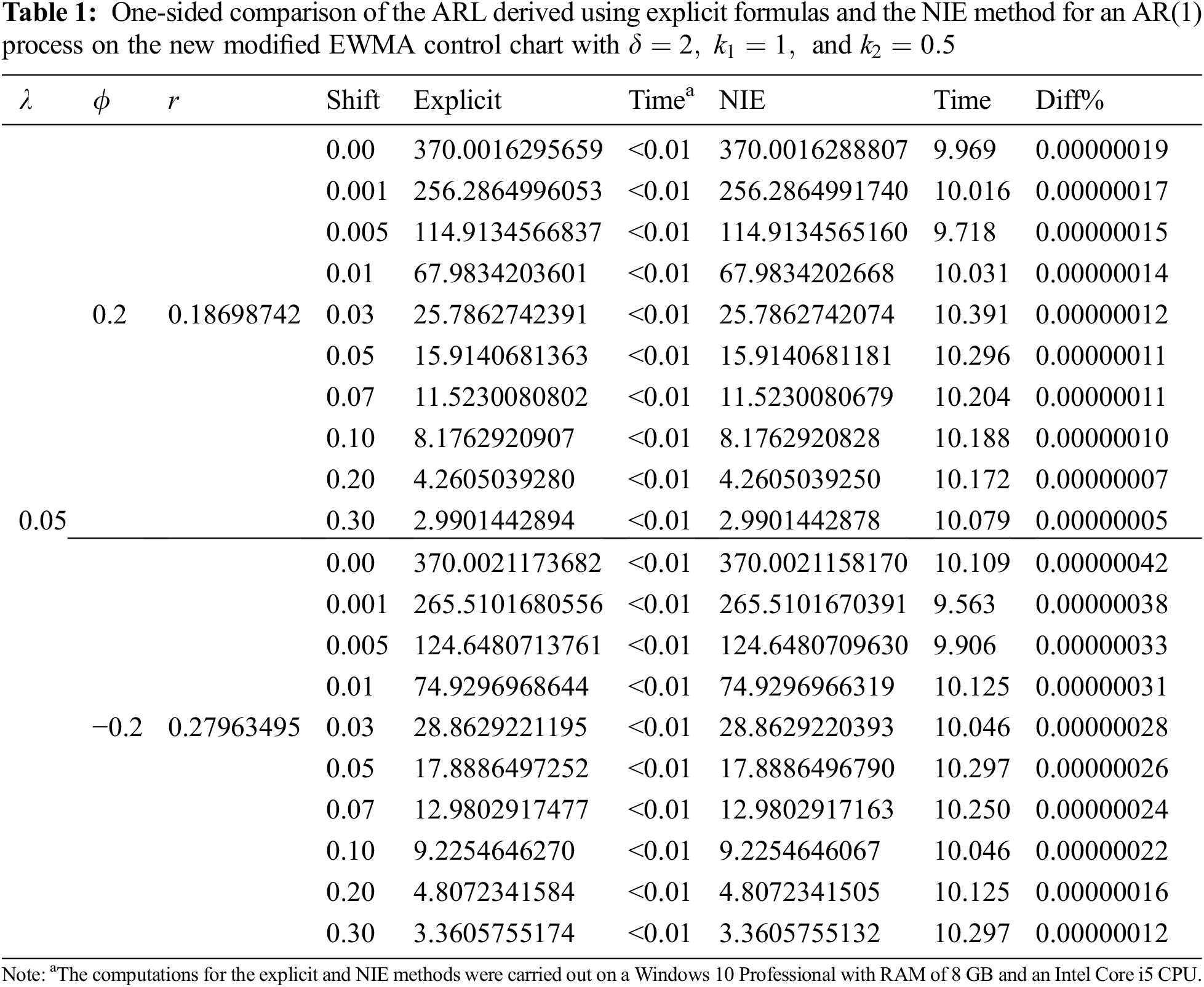
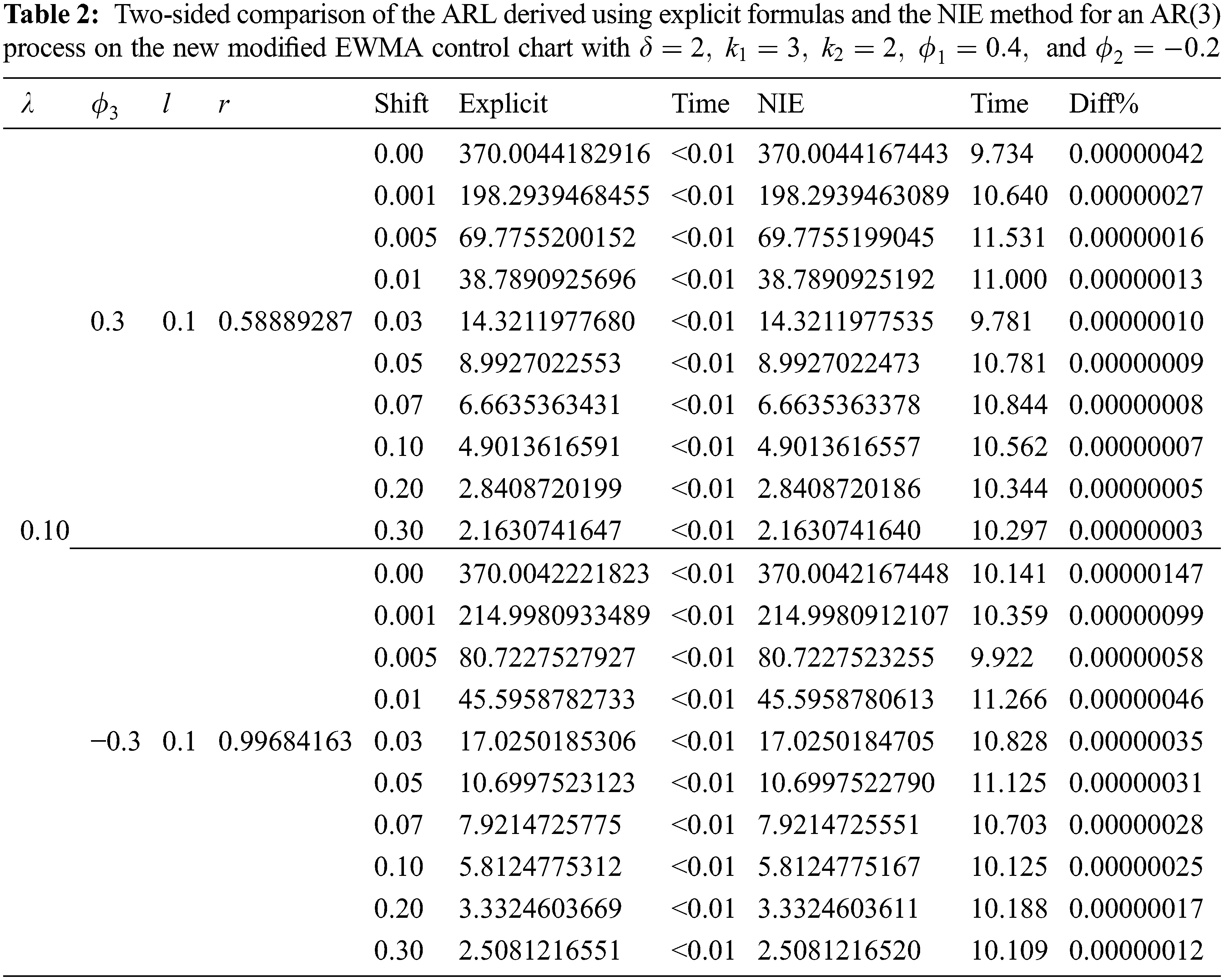
From the results in Tabs. 1 and 2, we can see that the ARL values derived by using the explicit formulas were the same as those of the NIE method, with the numerical approximations having an absolute percentage difference of less than 0.00001%. However, the computational time for the NIE method was 9.563 s–11.531 s whereas that for the explicit formulas was less than 1 s.

6  Comparison of the ARL Derived Using Explicit Formulas

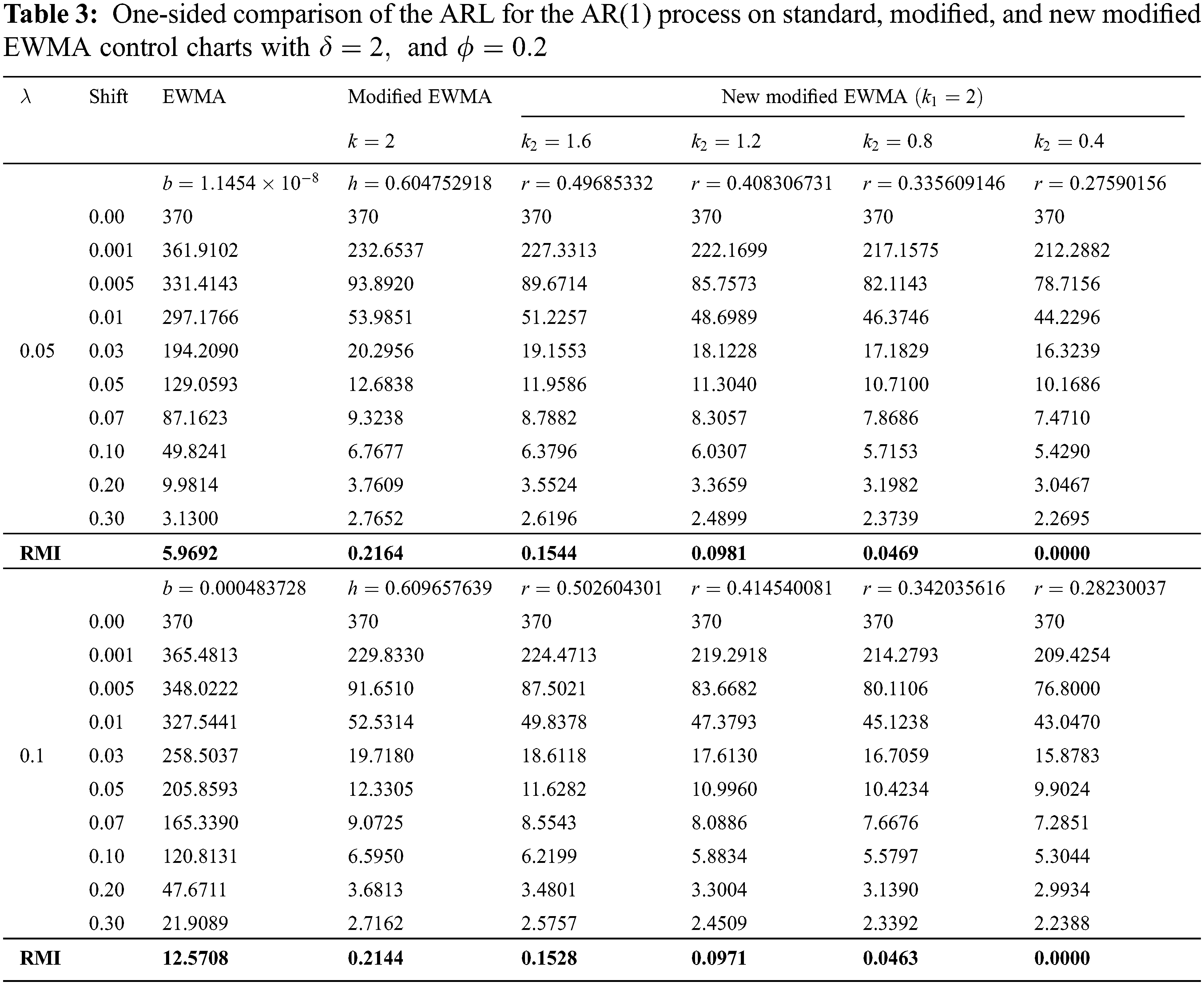
After verifying the accuracy of the explicit formulas, we used simulated data and the relative mean index (RMI) to compare the performances of the ARL derived using explicit formulas for an AR(p) process on standard, modified, and new modified EWMA control charts. The RMI is defined as

RMI(r)=1n∑i=1n(ARLi(r)−Min[ARLi(s)]Min[ARLi(s)]), (32)

where ARLi(r) is the ARL of the control chart for the shift size in row i and Min[ARLi(s)] denotes the smallest ARL of the three control charts in comparison to the shift size in row i, for i=1,2,…,n . The control chart with the smallest RMI is the best at detecting changes in the process mean for a particular set of criteria.

For the one-sided comparison of the ARL for an AR(1) process on the standard, modified, and new modified EWMA control charts, the parameter values were set as ARL0=370 ; λ= 0.05 or 0.1; in-control parameter α0=1 ; and a shift size of 0.001, 0.005, 0.01, 0.03, 0.05, 0.07, 0.1, 0.2, or 0.3. The results are reported in Tab. 3.

For the two-sided comparison of the ARL for an AR(2) process on the three control charts, the parameter values and the shift sizes were the same as for the one-sided comparison. The results are reported in Tab. 4.

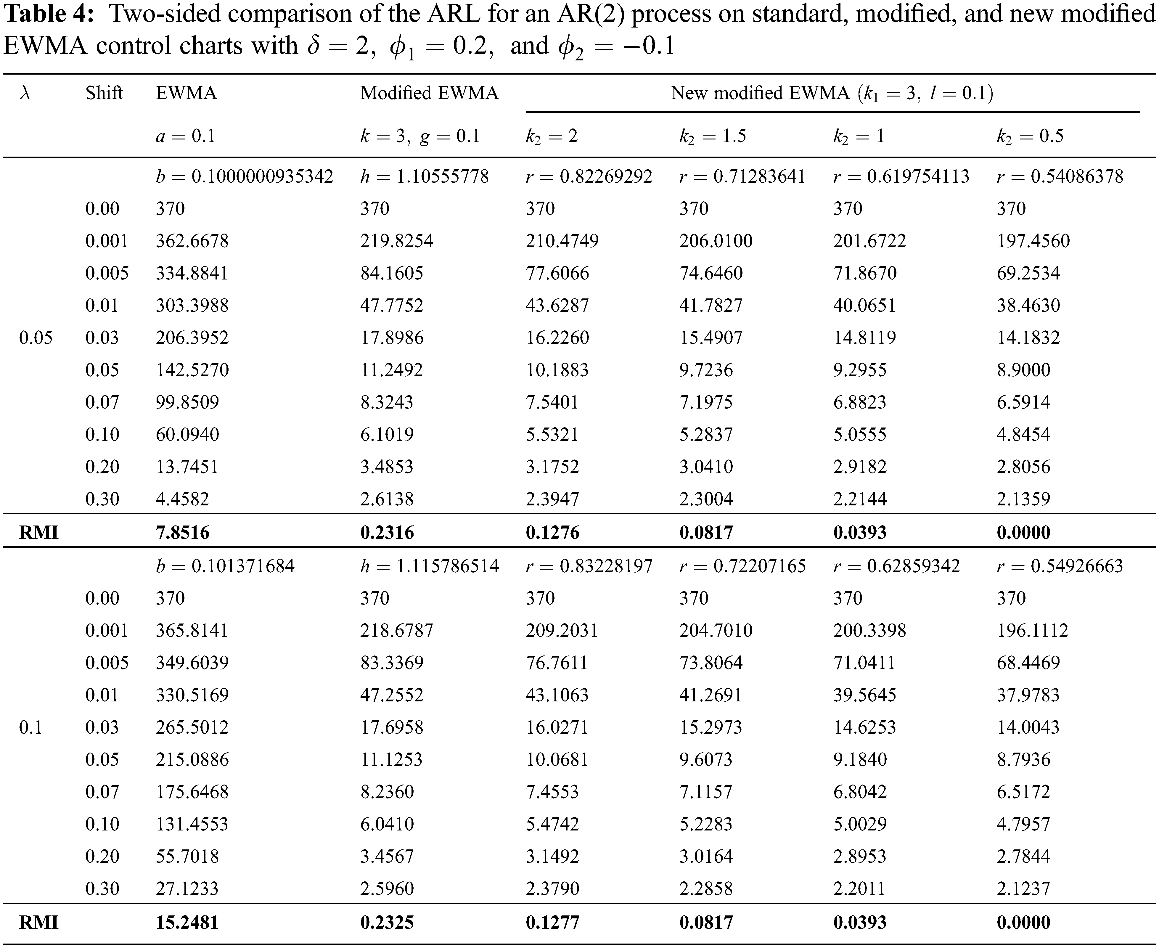
From the results in Tabs. 3 and 4, it is evident that the ARL values derived by using the explicit formulas for the new modified EWMA control chart are smaller than those for the standard and modified EWMA control charts for all shift sizes and λ for k1>k2 , and thus the RMI values of the ARL on the new modified EWMA control chart were smaller than those for the standard and modified EWMA control charts for all λ .

The property of the new modified EWMA control chart ensured that the ARL decreased as k1 was increased for k1>1 , and so the ARL value obtained by using the explicit formulas for the new modified EWMA control chart was lower than those for the standard and modified EWMA control charts under each set of conditions. For k2<k1 , the ARL value decreased as k2 became smaller (i.e., the importance of the historical information was reduced), which made the new modified EWMA control chart more efficient at detecting changes than the standard and modified EWMA control charts. Finally, the ARL was reduced as λ was increased.

7  Practical Applications

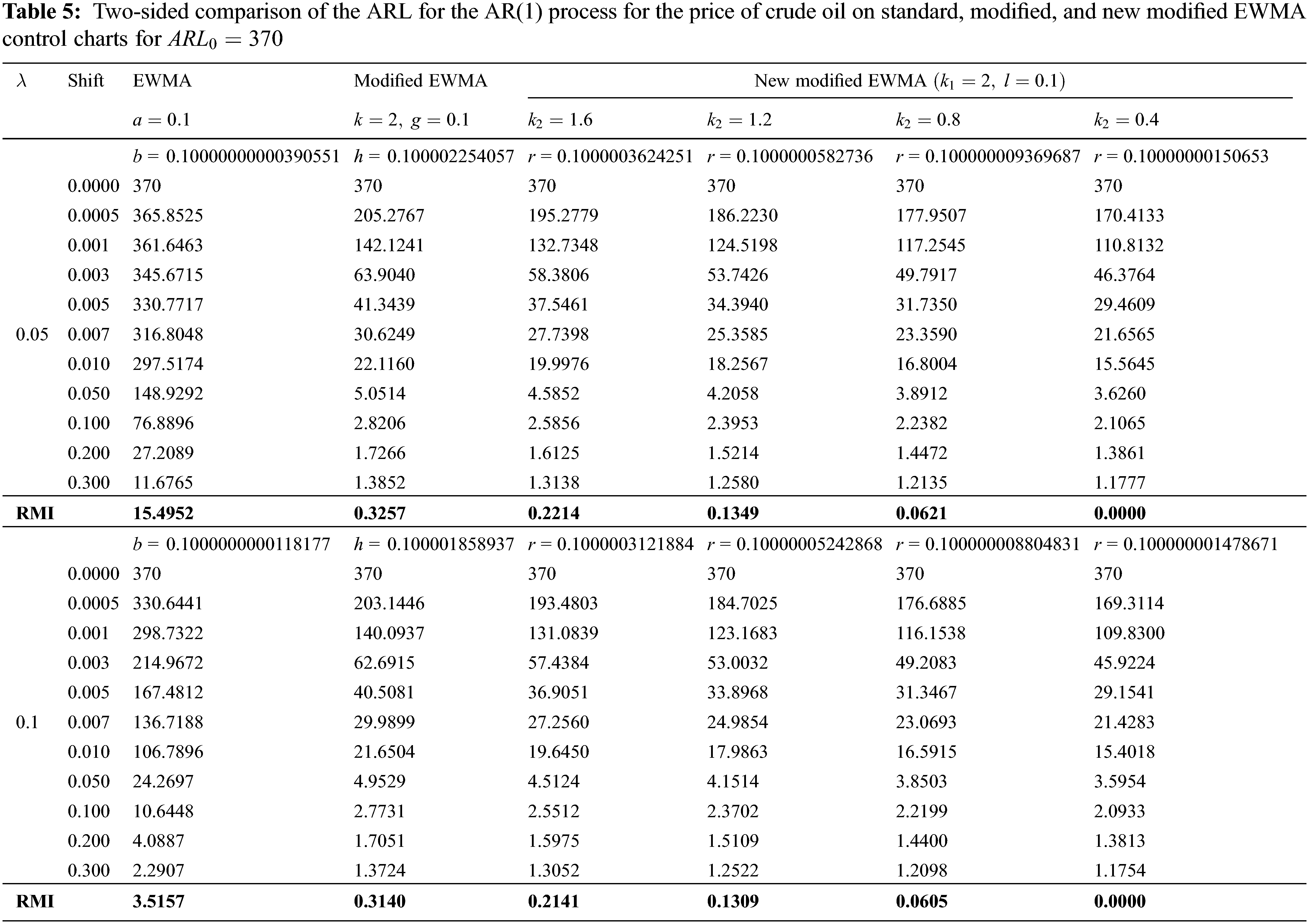
To confirm the results of the simulation study, we applied the explicit formulas for the ARL of an AR(1) process involving 72 real data observations of the price of crude oil (Unit: US Dollars per barrel) from January 2015 to December 2020 (data from the West Texas Intermediate [20]) on the standard, modified, and new modified EWMA control charts. The parameters were set as λ= 0.05 or 0.1; α0=3.2028 ; δ=50.6834 ; ϕ1=0.8750 ; and a shift size of 0.0005, 0.001, 0.003, 0.005, 0.007, 0.01, 0.05, 0.1, 0.2, or 0.3. The results are summarized in Tab. 5.

We also carried out another comparison for the ARL of an AR(2) process using 72 real data observations of the price of rubber (Unit: US Dollars per kilogram) from January 2015 to December 2020 (Singapore Exchange Ltd. (SGX) [21]) on the standard, modified, and new modified EWMA control charts. The parameters were set as λ= 0.05 or 0.1; α0=0.0989 ; δ=1.6660 ; ϕ1=1.2821 ; ϕ2=−0.4578 ; and a shift size of 0.00001, 0.00003, 0.00005, 0.00007, 0.0001, 0.0005, 0.001, 0.002, or 0.003. The results are summarized in Tab. 6.

From the results using real data in Tabs. 5 and 6, it is evident that the ARL values derived by using the explicit formulas for the new modified EWMA control chart were less than those for the standard and modified EWMA control charts for all shift sizes and λ for k1>k2 . This corresponds to the RMI values for the new modified EWMA control chart being less than those for the standard and modified EWMA control charts for all k2;k1>k2 . In addition, as k2 decreased, the ARL1 and the RMI decreased. Detection of shifts in the means of the AR(1) and AR(2) processes with real data on the three types of EWMA control charts are plotted in Figs. 1 and 2, respectively.

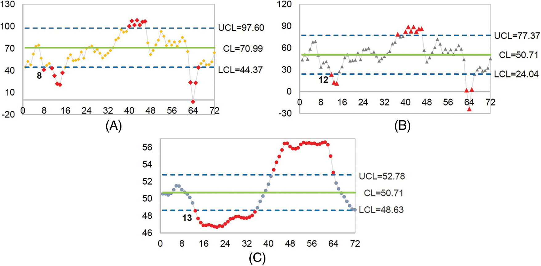
Figure 1: Mean shift detection for the AR(1) process for the price of crude oil. (A) The new modified EWMA control chart, (B) The modified EWMA control chart, and (C) The standard EWMA control chart

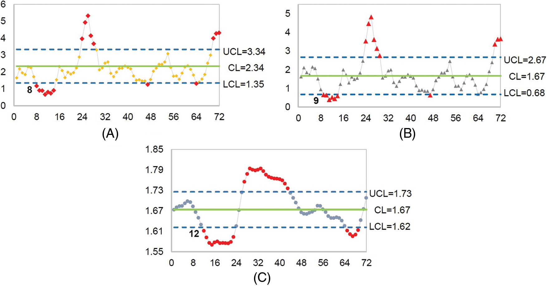
Figure 2: Mean shift detection of the AR(2) process for the price of rubber. (A) The new modified EWMA control chart, (B) The modified EWMA control chart, and (C) The standard EWMA control chart

The results in Fig. 1 indicate that the new modified EWMA control chart could detect a change in the price of crude oil for the first time at the 8th observation, while the standard and modified EWMA control charts achieved this at the 13th and 12th observations, respectively.

The results in Fig. 2 show that the new modified EWMA control chart could detect the price of rubber at the 8th observation for the first time whereas the standard and the modified EWMA control charts could only do so at the 12th and 9th observations, respectively. Hence, in both cases, detecting a shift in the process mean by the new modified EWMA control chart was sooner than either the standard or modified EWMA control charts, and therefore, it performed better.

8  Conclusions

A new modified EWMA control chart to detect a change in the process mean of an AR(p) process with exponential white noise was proposed. We derived explicit formulas for the ARL on the new modified EWMA control chart and checked its accuracy by comparing its absolute percentage difference with the widely used NIE method via a simulation study. The results show that although both methods were highly consistent with an absolute percentage difference of less than 0.00001%, the explicit formula method could be computed much more quickly. A comparison of the ARL derived by using explicit formulas on standard, modified, and new modified EWMA control charts shows that the proposed control chart was more efficacious than the others in terms of RMI. Application of the proposed control chart for AR(p) processes with exponential white noise using real data observations and a comparison of its performance with the standard and modified EWMA control charts show that the new modified EWMA control chart performed better than the others for a two-sided shift with all of the smoothing parameter values tested. In addition, as k2 decreased, its ARL1 and the RMI decreased. Based on the findings, the explicit formulas for the ARL of an AR(p) process with exponential white noise detected a change in the process mean more quickly on the new modified EWMA control chart than on the standard and modified EWMA control charts. Although the conclusions drawn from the results of this study are only applicable to AR(p) processes, it would be interesting to discover whether our approach is relevant for others, especially where autoregression is involved.

Acknowledgement: We are grateful to the referees for their constructive comments and suggestions which helped to improve this research.

Funding Statement: Thailand Science Research and Innovation Fund, and King Mongkut’s University of Technology North Bangkok Contract no. KMUTNB-FF-65–45.

Conflicts of Interest: The authors declare that they have no conflicts of interest to report regarding the present study.

Appendix A. The Mean and the variance of the new modified EWMA control chart

The new modified EWMA control chart based on the modified EWMA control chart proposed by Khan et al. [9] from Eq. (13) is defined as

Nt=(1−λ)Nt−1+λYt+k1Yt−k2Yt−1;t=1,2,3,…,

where k1 and k2 are constants ( k1>k2>0 ).‏

The mean of the new modified EWMA control statistic is E(Nt)=[λ+k1−k2]μ0λ . It may be shown that

Nt=(1−λ)Nt−1+λYt+k1Yt−k2Yt−1

=(1−λ)3Nt−3+(1−λ)2[λYt−2+k1Yt−2−k2Yt−3]+(1−λ)[λYt−1+k1Yt−1−k2Yt−2]+λYt+k1Yt−k2Yt−1

=(1−λ)3Nt−3+λ(1−λ)2Yt−2+λ(1−λ)Yt−1+λYt+(1−λ)2k1Yt−2+(1−λ)k1Yt−1+(1−λ)0k1Yt−(1−λ)2k2Yt−3−(1−λ)k2Yt−2−(1−λ)0k2Yt−1,

and continuing like this recursively for Yt−j;j=1,2,3,…,t , we obtain

Nt=(1−λ)tN0+∑j=0t−1(1−λ)j[(λ+k1)Yt−j−k2Yt−j−1]

Hence, ∑j=0t−1(1−λ)j[(λ+k1)Yt−j−k2Yt−j−1] accounts for sum of the past and latest change in the process.

The unaccounted current fluctuations accumulated to time t in new modified EWMA statistic.

Let Nt=(1−λ)tN0+∑j=0t−1(1−λ)j[(λ+k1)Yt−j−k2Yt−j−1] .

Take the expectation on both sides, we have

E(Nt)=(1−λ)tE(N0)+∑j=0t−1(1−λ)jE[(λ+k1)Yt−j−k2Yt−j−1]

=(1−λ)tμ0+[1−(1−λ)t1−(1−λ)][(λ+k1)μ0−k2μ0]=μ0+1λ[k1μ0−k2μ0];t→∞

=[λ+k1−k2]μ0λ

And the variance is Var(Nt)=[(λ+k1)2+k22−2λk2+2λ2k2−2k1k2+2λk1k2λ(2−λ)]σ2 . The derive of the variance of Nt is

Nt=(1−λ)tN0+(λ+k1)∑j=0t−1(1−λ)jYt−j−k2∑j=0t−1(1−λ)jYt−j−1

Var(Nt)=(1−λ)2tVar(N0)+(λ+k1)2∑j=0t−1(1−λ)2jVar(Yt−j)+k22∑j=0t−1(1−λ)2jVar(Yt−j−1)+2(λ+k1)(−k2)Cov[∑j=0t−1(1−λ)jYt−j,∑j=0t−1(1−λ)jYt−j−1]

=(1−λ)2tσ2+(λ+k1)2∑j=0t−1(1−λ)2jσ2+k22∑j=0t−1(1−λ)2jσ2−2(λ+k1)k2∑j=0t−1(1−λ)2j+1Cov(Yt−j,Yt−j−1)

=(1−λ)2tσ2+(λ+k1)2σ2[1−(1−λ)2tλ(2−λ)]+k22σ2[1−(1−λ)2tλ(2−λ)]−2(λ+k1)k2∑j=0t−1(1−λ)2j+1ρσσ

=[(λ+k1)2λ(2−λ)+k22λ(2−λ)−2(λ+k1)k2(1−λ)λ(2−λ)]σ2

when t→∞,ρ→1

=[λ2+2λk1+k12+k22−2λk2+2λ2k2−2k1k2+2λk1k2λ(2−λ)]σ2

Therefore, the mean and the variance of the new modified EWMA control chart are respectively defined as

E(Nt)=(λ+k1−k2)μ0λ , and Var(Nt)=[(λ+k1)2+k22−2λk2+2λ2k2−2k1k2+2λk1k2λ(2−λ)]σ2.

References

1. I. Madanhire and C. Mbohwa, “Statistical process control (SPC) application in a manufacturing firm to improve cost effectiveness: Case study,” in Proc. IOEM 2016, Kuala Lumpur, KL, Malaysia, pp. 2298–2305, 2016. [Google Scholar]
2. W. A. Shewhart, Economic Control of Quality of Manufactured Product, New York, NY, USA: D. Van Nostrand Company, 1931. [online]. Available: https://dspace.gipe.ac.in/xmlui/bitstream/handle/10973/18338/GIPE-009900.pdf?sequence=3. [Google Scholar]
3. E. S. Page, “Continuous inspection schemes,” Biometrika, vol. 41, no. 1/2, pp. 100–115, 1954. [Google Scholar]
4. D. M. Hawkins and D. H. Olwell, Cumulative Sum Charts and Charting for Quality Improvement, New York, NY, USA: Springer, 1998. [online]. Available: https://link.springer.com/book/10.1007/978-1-4612-1686-5. [Google Scholar]
5. D. R. Prajapati, “Effectiveness of conventional CUSUM control chart for correlated observations,” International Journal of Modeling and Optimization, vol. 5, no. 2, pp. 135–139, 2015. [Google Scholar]
6. S. W. Roberts, “Control chart test based on geometric moving average,” Technometrics, vol. 1, no. 3, pp. 239–250, 1959. [Google Scholar]
7. S. V. Crowder, “A simple method for studying run length distributions of exponentially weighted moving average charts,” Technometrics, vol. 29, no. 4, pp. 401–407, 1987. [Google Scholar]
8. J. M. Lucas and M. S. Saccucci, “Exponentially weighted moving average control schemes: Properties and enhancements,” Technometrics, vol. 32, no. 1, pp. 1–12, 1990. [Google Scholar]
9. N. Khan, M. Aslam and C. -H. Jun, “Design of a control chart using a modified EWMA statistic,” Quality and Reliability Engineering International, vol. 33, pp. 1095–1104, 2016. [Google Scholar]
10. A. K. Patel and J. Divecha, “Modified exponentially weighted moving average (EWMA) control chart for an analytical process data,” Journal of Chemical Engineering and Materials Science, vol. 2, no. 1, pp. 12–20, 2011. [Google Scholar]
11. S. M. Anwar, M. Aslam, S. Ahmad and M. A. Riaz, “A modified-mxEWMA location chart for the improved process monitoring using auxiliary information and its application in wood industry,” Quality Technology & Quantitative Management, vol. 17, no. 5, pp. 561–579, 2020. [Google Scholar]
12. M. Aslam and S. M. Anwar, “An improved Bayesian modified EWMA location chart and its applications in mechanical and sport industry,” PLOS ONE, vol. 15, no. 2, e0229422, 2020. [Google Scholar]
13. Y. Areepong, “An integral equation approach for analysis of control charts,” Ph.D. dissertation, University of Technology, Sydney, Australia, 2009. [Google Scholar]
14. C. W. Champ and S. E. Rigdon, “A comparison of the markov chain and the integral equation approaches for evaluating the run length distribution of quality control charts,” Communications in Statistics-Simulation and Computation, vol. 20, no. 1, pp. 191–204, 1991. [Google Scholar]
15. T. J. Harris and W. H. Ross, “Statistical process control procedures for correlated observations,” Canadian Journal of Chemical Engineering, vol. 69, no. 1, pp. 48–57, 1991. [Google Scholar]
16. L. VanBrackle and M. R. Reynolds, “EWMA and CUSUM control charts in the presence of correlation,” Communications in Statistics-Simulation and Computation, vol. 26, pp. 979–1008, 1997. [Google Scholar]
17. G. Mititelu, Y. Areepong, S. Sukparungsee and A. Novikov, “Explicit analytical solutions for the average run length of CUSUM and EWMA charts,” Contribution in Mathematics and Applications III East-West J. of Mathematics,, a special volume, pp. 253–265, 2010. [Google Scholar]
18. S. P. Richard, “A simple proof of the banach contraction principle,” Journal of Fixed-Point Theory and Applications, vol. 2, pp. 221–223, 2007. [Google Scholar]
19. P. Phanthuna, Y. Areepong and S. Sukparungsee, “Numerical integral equation methods of average run length on modified EWMA control chart for exponential AR(1) process,” in Proc. IMECS 2018 Vol II, Hong Kong, HK, pp. 845–847, 2018. [Google Scholar]
20. IndexMundi. The price of crude oil. 2021. “Dryad digital repository,” [online]. Available: https://www.indexmundi.com/commodities/?commodity=crude-oil-west-texas-intermediate&months=120. [Google Scholar]
21. IndexMundi. The price of rubber. 2021. “Dryad digital repository,” [online]. Available: https://www.indexmundi.com/commodities/?commodity=rubber&months=120. [Google Scholar]