Multi-Level Deep Generative Adversarial Networks for Brain Tumor Classification on Magnetic Resonance Images

1  Introduction

In the current age, many computer vision and image processing techniques have substantially influenced medicinal image examination and diagnosis to achieve the results of competent medical experts [1,2]. The development of computer-aided systems and deep learning techniques in the medical field has become the most prominent research area to meet the current age challenges in different medical fields. Although medical imaging data is increasing day by day, with an increasing number of robust systems, newly developed techniques are the main backbone to executing the success of different deep neural networks [3].

Brain tumors (BT) occur due to brain cells’ hysterical and atypical evolution [4]. There are many types of brain tumors, but the most common is glioma tumor (GT). The GT occurs due to glial cells in the central nervous system responsible for handling the nutritional elements of a human brain [5]. Moreover, meningioma, the word originated from three membranes surrounding the brain and spinal cord. It originates in these membranes [6]. The pituitary is a small gland located at the back of the nose. Its irregular growth affects other brain glands and many functions in the body [7].

Additionally, medical imaging-related applications are increasing daily to facilitate the medical experts [8]. The convolutional neural networks (CNNs) have been applied to increase radiology practice efficiency, elastic registration between 3D MRI images, separation of brain tumors, neuropsychiatric illnesses, cancer in the breast, and medically ultrasound-based images [9].

The classification of brain tumorous MRI is the latest research topic centered on many deep learning techniques for qualitative analysis of brain tumors [10]. According to medical experts, brain tumor is one of the dangerous diseases that leads to the maximum number of deaths of all ages [11]. That’s why the accurate diagnosis process of BT during the curing process is crucial and needs a maximum level of specialization for medical experts to complete the diagnosis process. So, a Generative Adversarial Network (GAN) is prosed to handle this challenge.

On the other hand, the proposed technique known as GAN is the well-known machine learning technique consisting of two neural networks contended with each other to be most accurate in prediction results [12]. The GAN network consists of the generator model and discriminator model. The generator is the CNN, and the discriminator is the de-convolutional neural network. The generator’s function is to create the output artificially, while the discriminator is used to verify the artificially created output by the generator. GAN creates its training data to generate the higher quality output for text to image translation, image editing, creating and recreating with higher resolution, and 3-D object creation. Conversely, the discriminator model grows into a better network to verify the artificially created output [13].

Identifying the desired end product and collecting an original training dataset depends on those parameters is the initial phase in creating a GAN network. The achieved information known as random input is fed into the generator till it reaches a baseline level of resultant output. After that, these features are fed up with discriminators with authentic data points. The discriminator analyses the authenticity of each image data and produces a probability between 1 and 0 for true and fake correlates [14]. The achievement of these results is manual-based checking, and the method is repetitive till the preferred outcomes are achieved, as shown in Fig. 1.

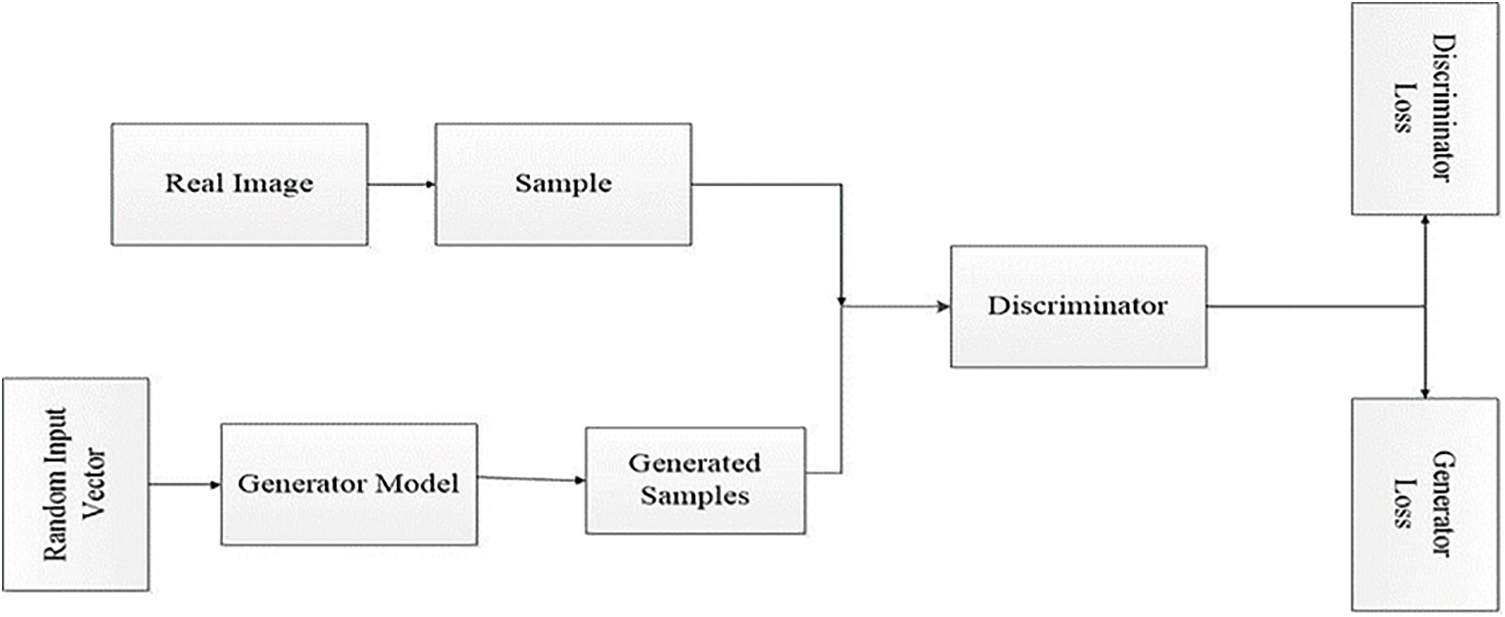
Figure 1: General GAN network architecture

As a contribution to our proposed work for brain tumor classification, this research presented a new strategy known as the GAN network. The contributions of the proposed work are given below:

•   The GAN network created artificial medical image data to improve the learning ability of physicians and other computer-aided systems for the generation of augmented data.

•   GAN network initially goes through a training process on different MRI images to generate realistic images of brain tumors that are entirely altered from the original ones.

The remaining paper structure is presented as the second part presents the interrelated work, the third part explains the overall methodology, fourth one describes the experimental-based results and discussions, and the last section indicates the conclusion of the whole research work.

2  Related Work

Along with other traditional methods [15], CNNs [16,17] have a prominent role in medicinal image-based analysis, including brain segmentation of magnetic resonance images (MRIs) [18]. MR imaging consists of harmful ionizing radiations, but these radiations do not affect the patients and provide information related to the brain tumor’s size, shape, type, and position. Glioma and meningioma are the two hazardous types of brain tumors (BTs) detected by MRI scans. If these BTs are not detected initially, they can be very dangerous and lead to death [19].

Glioma is the famous type of BTs in humans worldwide [20]. The famous institute, known as the World Health Organization (WHO), categorizes the tumor into four grades. Grade I and II is the lower level of brain tumor known as meningioma, and grade III and IV is identified as a more severe type of tumor-like glioma [21]. More or less 20% is the meningioma type of brain tumor and treated as slowest in growth. The initial stage diagnosis of this type of tumor can save many people’s lives [22].

The interpretation of MRIs by trained medical experts of brain tumorous disease is a considerably more time-consuming, sensitive, and complicated job. In many cases, the brain tumor size is slightly different in color concentration, form, and surface [23]. Noisy images and fewer concentration factors for the trained medical expert are the other two issues for misinterpretation of brain tumors. Therefore the correct decision about the diagnosis of BT is a much more challenging task for the trained neurologists and surgeons [24].

On the other hand, the author applied three classifiers known as CNN, random forest classifier, and fully connected neural network for the brain tumor analysis in [25]. The best accuracy obtained by CNN is 90.26%. In this technique, the CNN consists of different parameters such as convolutional, fully connected, and pooling layers for the identification process [26]. Moreover, a capsule net was used to organize three brain tumors fed with MRI images. The classification accuracy obtained is 86.56% with the segmentation process and 72% with new brain tumor MRIs [27].

A Generative Adversarial Networks (GANs) was presented in the paper [28], which contains two nets first one is a generator known as a convolutional neural network, and the second one is a discriminator famous as a deconvolutional neural network. The generator attempts to yield actual output created on real distributed data to step out of the discriminator model. It is used to differentiate the actual data as generated by the generator. Moreover, the generator produces more real output and discriminator tries to create the most realistic copies of accurate data during the training process [13].

In another work, GAN was used to produce realistic images of faces, buildings, and other places that were not easily detected by human eyes [29]. GAN was used for the semantic BT segmentation extensively [30]. Consequently, the segmented process is used as a generator, and the discriminator is used to construct the additional GANs [31]. The discriminator delivers the fractional reality of the data without labels in the unsupervised learning process [32]. In another research, deep CNN used a deep convolution-based GAN for both generator and discriminator models.

Most of the researchers used data augmentation techniques [33] to enhance the quantity of the dataset. These techniques based on the GAN network create realistic data but almost new sample images to enhance the performance [28]. These newly created data images cover the place of accurate data, which is used to increase the output accuracy [12]. The GAN network is also used for classification facilitation [34,35], object detection [36,37], and separation [38] to handle the deficiency of trainable data images.

Additionally, adversarial learning is also used for medicinal imaging for genuine retinal and computed tomography image creation to enhance the output values [39,40]. A recent study shows a valuable performance for liver classification by using CNN based technique for GAN training data [41]. However, GAN-based MRI image generation is not so far appropriate because of low contrast MRI images and intra-classification variations. In another work, the author generated 64 × 64/128 × 128 MRIs by using conventional GANs even medical experts could not distinguish between real and synthetic images [42].

Recently, many researchers in medical imaging have begun to use the GAN network to generate the super-resolution images, anomaly detection, and estimation of computed tomography (CT) images from the related MR images [43]. Additionally, the generation of medical images from GAN as the realistic data augmentation GAN-based model is one of the best solutions for the training of physicians for MRI brain tumor images [44].

3  Methodology

The methodology section consists of the overall proposed methodology. A GAN is proposed in this work, which comprises two models known as generator and discriminator. The details of the applied methodology are given below.

3.1 Generator Model

The first model is recognized as a generator. It is also famous as ordinary CNN. The generator model creates a sample in the domain from a fixed-length random vector as input. The Gaussian distribution randomly draws vector space and seals it to the generative process. During the training process, the vectors in the vector space correspond to the respective points in the domain space and form the distribution map. After that, it creates the random latent space variables which we cannot directly observe.

During the example of GAN, the generator allots sense to topics in a specified latent space, letting new facts pinched from the same space be delivered as the input and applied to yield new and various output samples. It attempts to yield actual output based on accurate spread data to mislead the discriminator. It is used to differentiate the actual data produced by the generator, as shown in Fig. 2a.

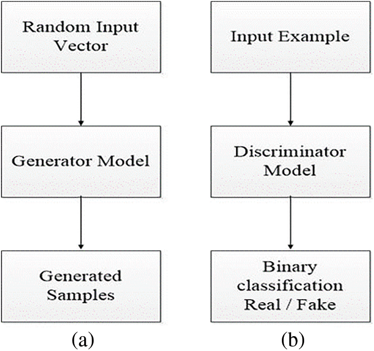
Figure 2: Representation of generator model (a) and discriminator model view (b)

The generator model behaves like an ordinary CNN. The presented CNN model have own architecture and working environment. The generator takes input as random sample and produces new samples. This workflow uses seventeen layers to generate the generator model. The first layer is the input and image size is known by setting the channel’s weight, height, and size. The kernel size, the network’s learning rate, and stride are indicated using the convolution layer as shown in Eq. (3).

For the swiftness of the network, a batch normalization layer is fed to the framework. On the other hand, an activation function is added in the form of the rectified linear unit (ReLU) as presented in Eq. (1). More input is distributed into numerous pooling sections, and the max-pooling layer calculates the peak value for every region. The overall structure of the used layers is presented in Tab. 1 and Fig. 3 using various constraints and kernel dimensions that vary from 4 to 16, and the learning rate value is 0.001 with an epoch value of 50. Subsequently, the fully connected layer pools all the yields of earlier layers; in other words, it chains all the learned characteristics of the layers to acknowledge the enormous configurations as revealed in Eq. (2). Additionally, the softmax layer works as an activation function for normalization. By applying the possibilities, the classification layer categorizes it into stated classes.

f(a) = {0, for  b <0b,for  b≥0  (1)

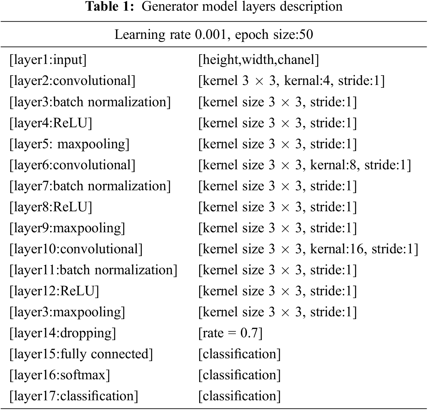
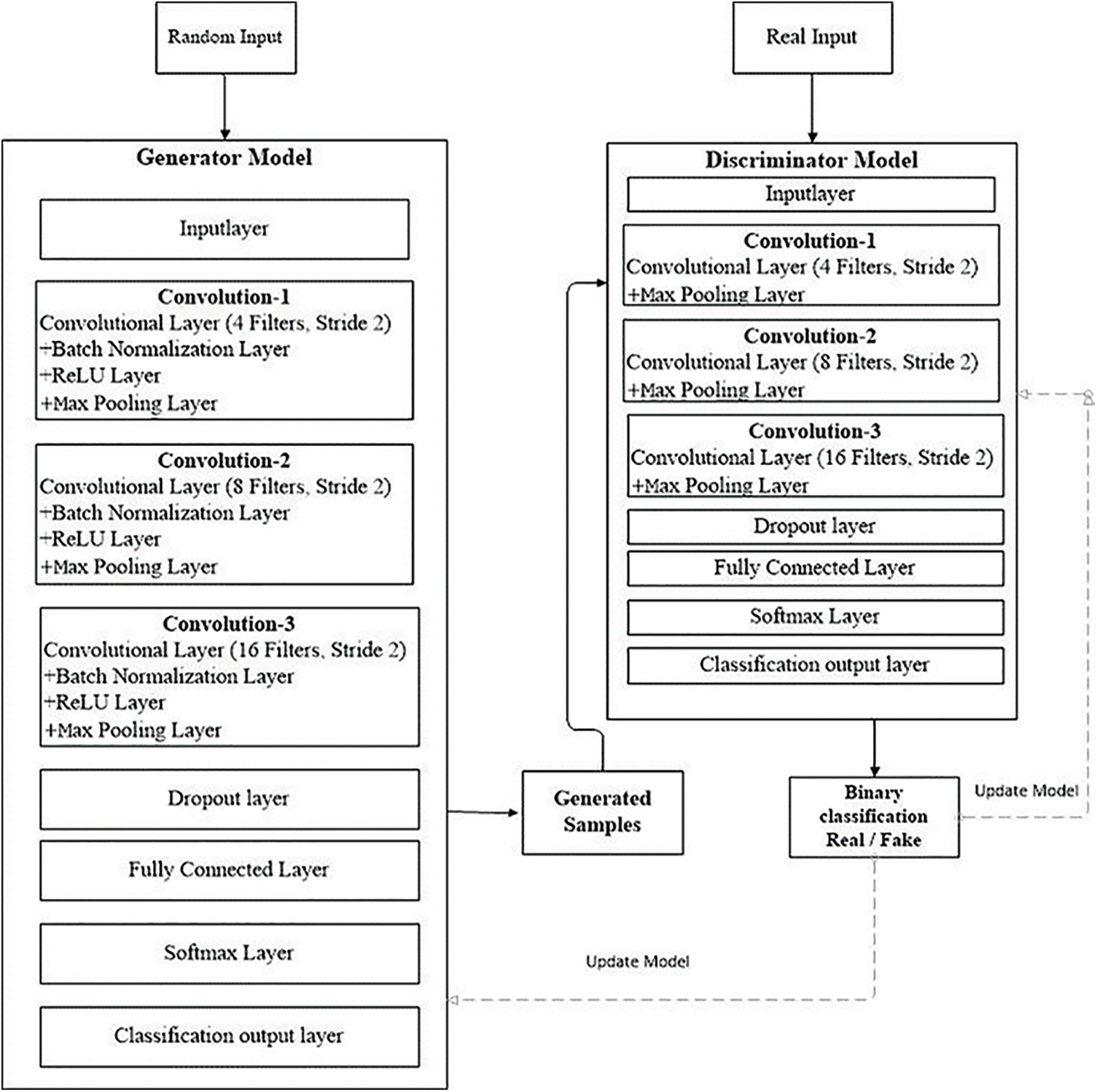
Figure 3: GAN model workflow

Here, f (a) is the ReLU layer functionality and b the target value as revealed in Eq. (1).

fc=rcF(fc−1)=((fc−1))twic+ac (2)

In Eq. (2), fc show the output of fully connected net, F is the number of filters r the input, w weight and a indicate the constant.

c =(rd+2pa− fd)str +1 (3)

Here Eq. (3) is the convolutional layer c, rd is the dimension of input,  pa shows padding,  fd indicate the filter dimensions and str represent the stride.

3.2 Discriminator Model

The second part of the GAN model is known as the discriminator model. The function of the discriminator is used to verify the artificially created output by the generator. The discriminator model inputs a domain sample and forecasts a true or false binary class label .The real-world example is taken from the trainable dataset. The generator model only generates examples. A normal classification model is used as a discriminator. The discriminator model is discarded after training because the generator indicate the interesting space. As it has learned to abstract features from examples in the problematic domain, the generator can be repurposed in some cases. On the other hand, transfer learning programs can use similar or equal input data for all feature extraction layers, as shown in Fig. 2b.

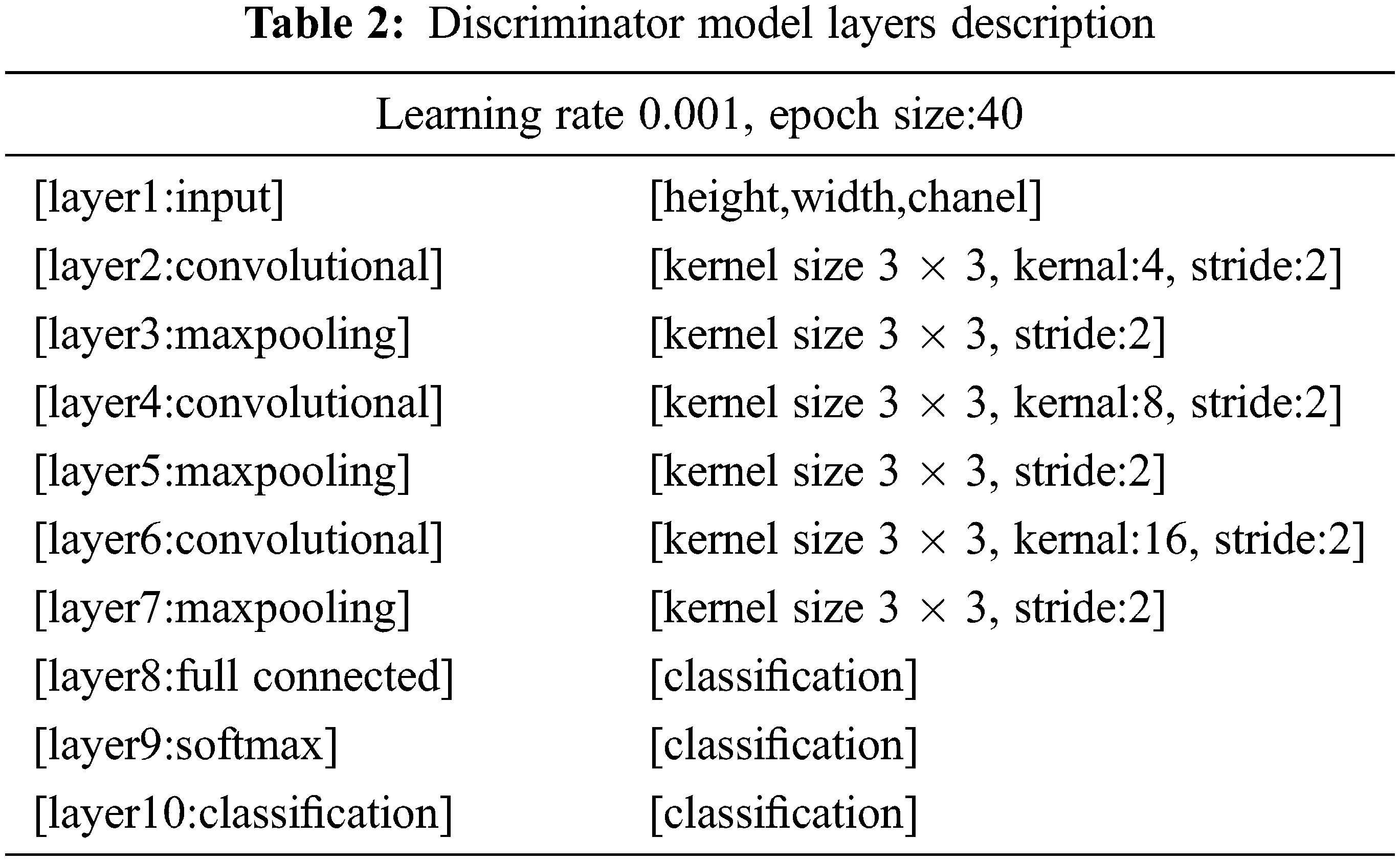
It behaves like an ordinary deconvolutional neural network. This model applied overall ten layers of CNN with various constraints and filters for the classification purpose. The number one layer is input layer having restrictions as weight, height, and size of the channel. In the convolutional layer number of filters, size and stride are defined, while the kernel values are specified from 4 to 16. Moreover, the learning rate for the training process is 0.001, with an epoch value of 40. The comprehensive layers explanation is given in Tab. 2, and workflow is also revealed in Fig. 3.

3.3 Overall Training Process

The workflow in Fig. 3 displays the complete training of the GAN network. At the initial level pre-trained CNN model is used as a discriminator in a GAN to distinguish real MRIs produced by the generative model from real ones. The discriminator can extract and learn the features of MRIs in this way. After that, pre-trained CNN is combined for brain tumor brain tumor classification. During the classification module, the last fully connected net is replaced with a softmax layer to enhance classification accuracy. GAN was accomplished to handle 8 to 64 batches for each brain tumor image. Every batch contains two pixel-wise mini-batch images. The first few images are from datasets of actual MRIs, while a few images are from a generator model with a randomized vector as input from a specific latent space. In this way, the generator generates some sample images. Additionally, the discriminator gets the real image as input, passes it through the deconvolutional model, and creates binary classification for real and fake images in the training and testing process as revealed in Fig. 3.

4  Results and Discussion

All the models in this research have been implemented by using Python (3.6.6) with supportive libraries as NumPy array (np), Keras models (2.2.4), layers and utils, matplotlib, sklearn utils and metrics, TensorFlow models, pandas, and seaborn. These libraries support the development of machine-learning applications. The proposed model was calculated on the system with Core i9 11th generation, Nvidia graphic card 6 GB, and 16 GB of RAM.

4.1 Dataset Details

The freely accessible CE-MRI dataset (https://figshare.com/articles/braintumor dataset/1512427) has been used. It consists of 2-dimensional images with a large slice gape. The dataset was collected from 2005 to 2020 from different hospitals in China. The dataset consists of four tumor classes: glioma, meningioma, pituitary, and no tumor [45], as revealed in Fig. 4. A glioma tumor is a common brain tumor that originates in the glial tissues surrounded by neurons [46].

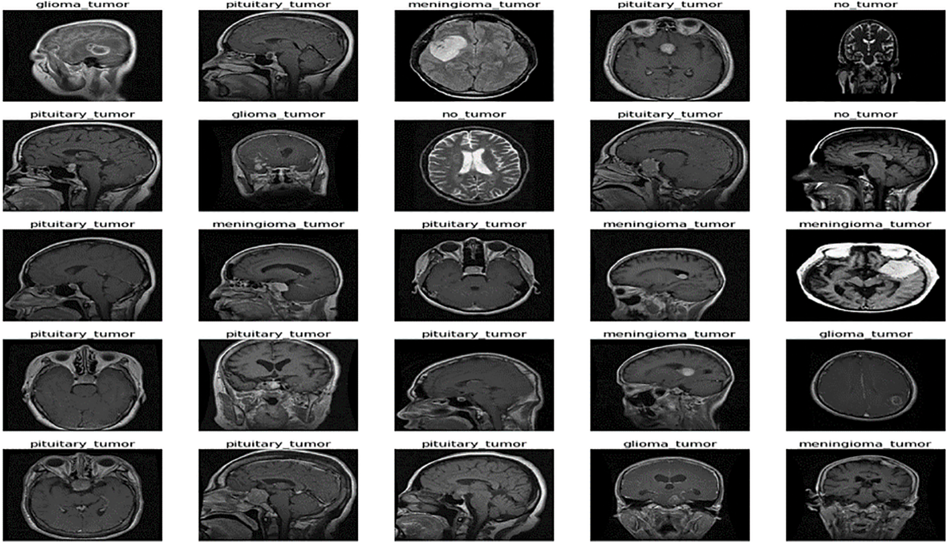
Figure 4: Sample images of CE-MRI dataset

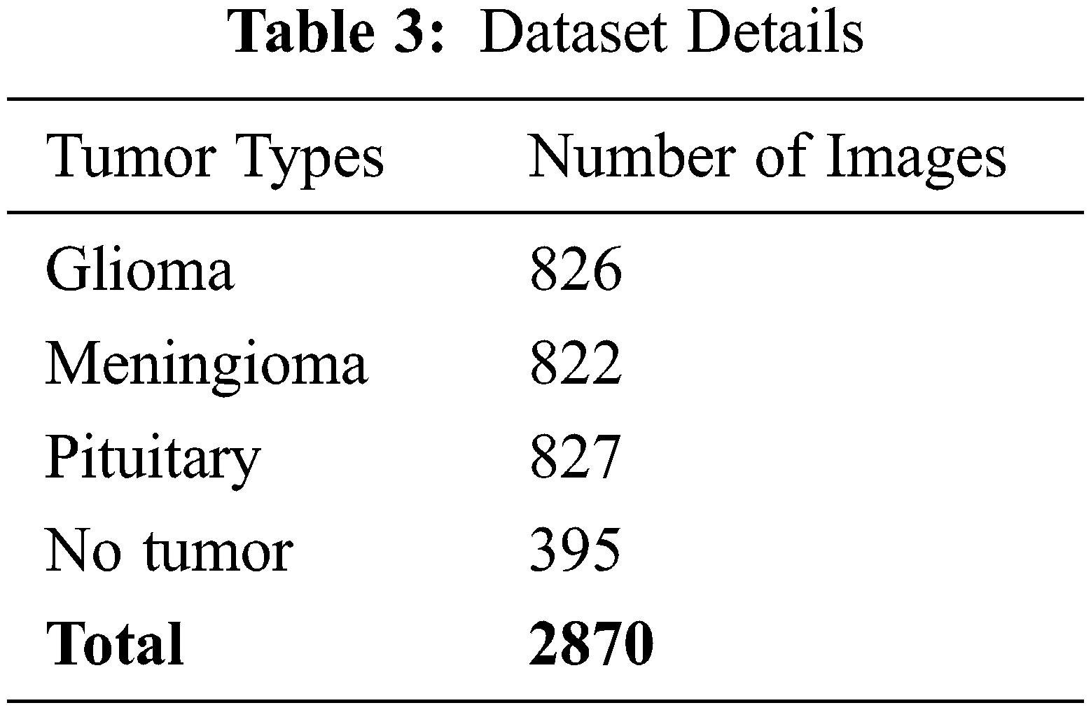
In contrast, meningioma is a tumor that arises from meninges tissues surrounding the brain and spinal cardinal system [47]. A pituitary tumor is due to the abnormal growth of pituitary glands in the back of the nose [48]. The size of each image in the dataset is 512 × 512 pixels, as shown in Fig. 2. The CE-MRI dataset was separated into training 70%, validation 15%, and testing 15%. The description of dataset is given below in Tab. 3.

4.2 Preprocessing

The images in the dataset are 2-dimensional with 512 × 512 pixels, as shown in Fig. 4. The dataset is checked with duplication, missing values, label name, and extension during the cleaning. Moreover, all the images are made noise-free using a histogram equalizer. In this work, the images are directly fed to the convolutional neural network, and the kernel is applied to resize the images. The results are highly dependent on these values. However, these values are not fixed and vary according to the image pixel sizes. To remove these intensity variations, normalization is used. So before giving values to the CNN model, all the values are normalized, having the same size range. Now the size of the images is 224 × 224 after normalization and resizing. In this way, the training process speeds up by resizing images and requires less memory.

4.3 Statistical Evaluations

The proposed GAN network for brain tumor classification and detection is calculated with the help of different arithmetical calculations specified underneath Eqs. (4)–(7). The correctly classified images are known tp, negatively true classified images are denoted as tn, while fp are the positively incorrect classified images. Moreover, fn represents the total number of negatively classified images. The statistical equations are given below:

Precision=tp(tp+fp) (4)

Recall=tp(tp+fn) (5)

F1−score=2(Sensitivity ×Precision)Sensitivity + Precision   (6)

Accuracy=(tp+tn)(tn+tp+fp+fn) (7)

4.4 Discussion

After completion of the training and testing process, the GAN network creates some fake images to enhance the dataset to increase the training of the model, as shown in Figs. 5A, 5B, 5C and 5D. Fig. 7 shows the GAN model confusion matrix for the four-class classification of the test dataset. The test dataset consists of four tumor classes glioma, meningioma, pituitary, and no tumor. On the other hand Fig. 6 shows the training process confusion Metrix. The numbers in the boxes of the confusion matrix show the overall number of images used for the classification purpose. Fig. 12 displays the graphical demonstration of accuracy and loss for training and validation. The statistical values are also shown in Tab. 2 with average precision: 0.92, recall: 0.93, F1-score: 0.93 and accuracy 0.98 values.

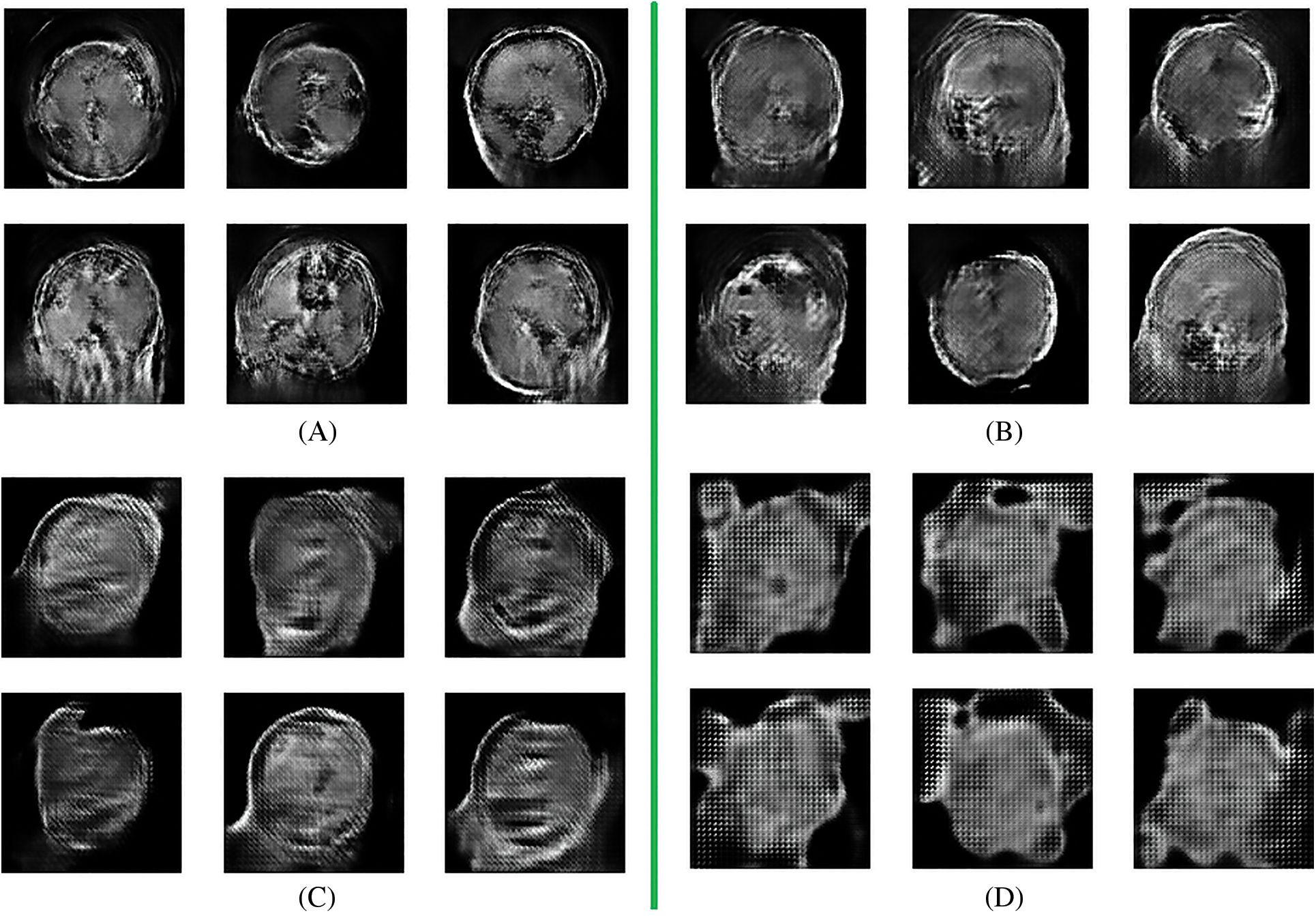
Figure 5: Fake data generation by GAN network (A) 8 batches (B) 16 batches (C) 32 batches (D) 64 batches

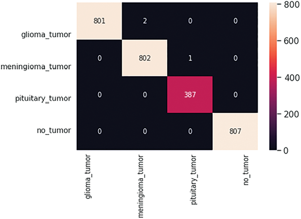
Figure 6: GAN model four-class classification confusion matrix for the training dataset

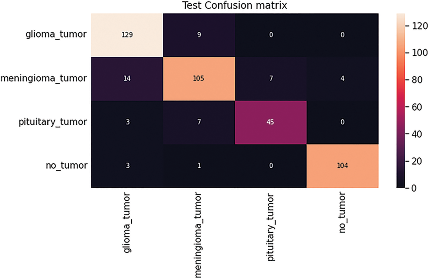
Figure 7: GAN model four-class classification confusion matrix for the test dataset

Figs. 8, 9, 10 and 11 shows the graphical demonstration using the GAN network’s 8, 16, 32, and 64 mini-batches. The y-axis depicts the loss, and the x-axis represents the GAN network simulation batch numbers. The blue line indicates the generator model evaluation. The orange line represents the discriminator model values and overlaps for some values.

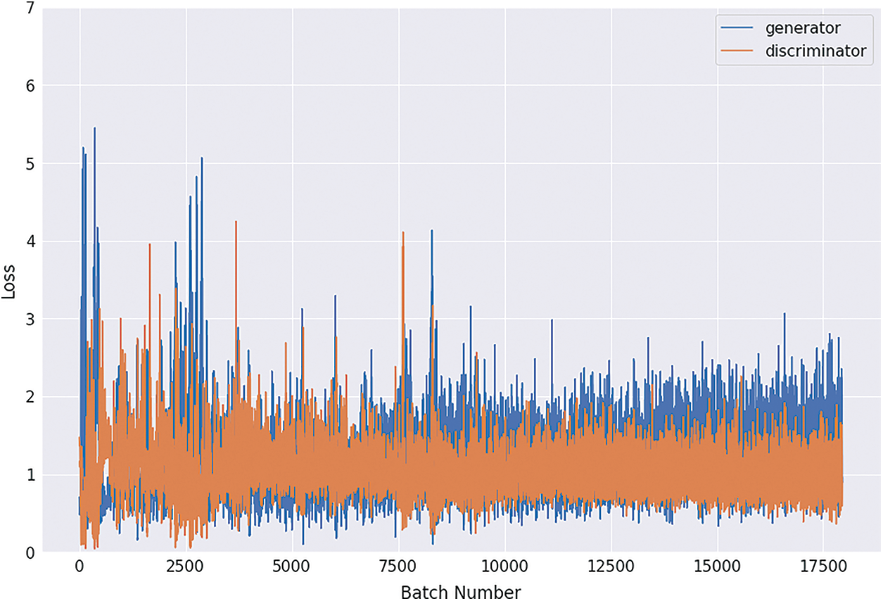
Figure 8: Graphical demonstration of 8 batches loss for GAN network

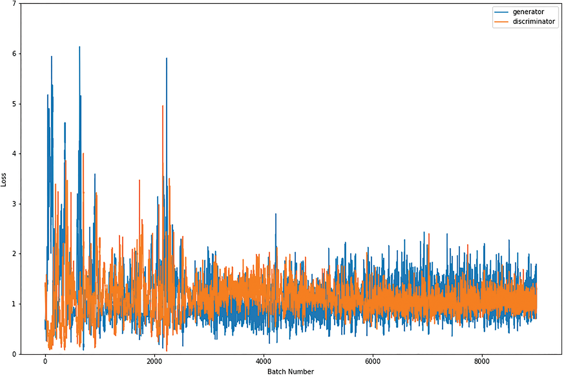
Figure 9: Graphical demonstration of 16 batches loss for GAN network

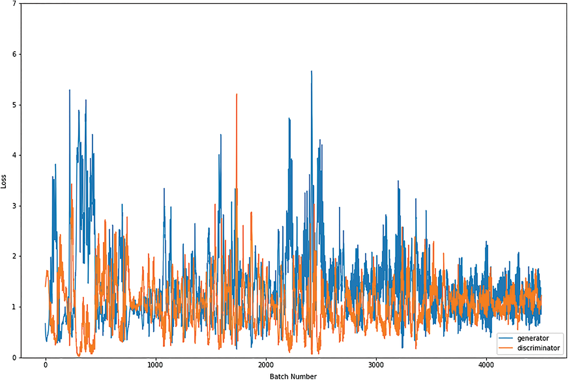
Figure 10: Graphical demonstration of 32 batches loss for GAN network

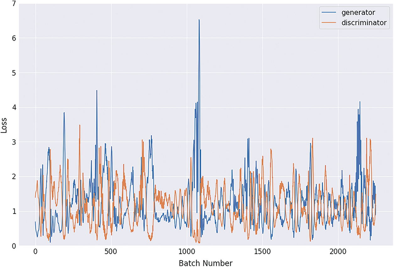
Figure 11: Graphical demonstration of 64 batches loss for GAN network

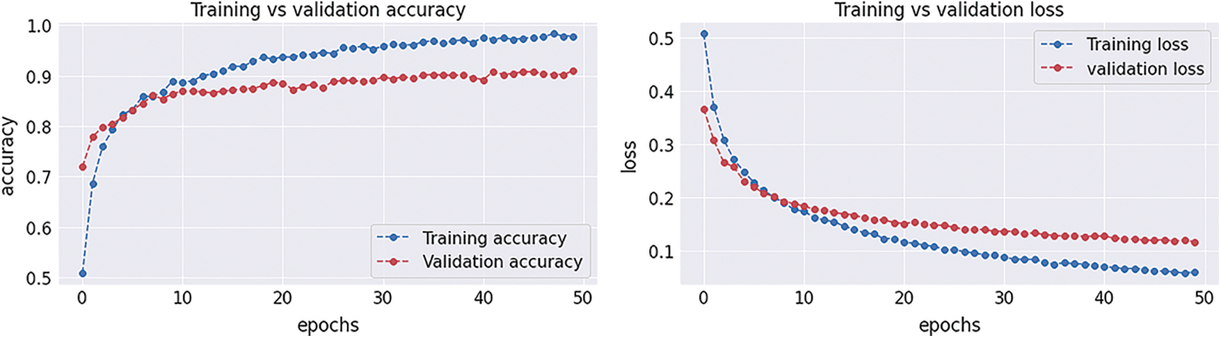
Figure 12: Graphical demonstration of training and validation accuracy and loss

During the simulation process, the batch number increases up to 17500 with almost 5.5 percent loss for 8 batch size simulation, as shown in Fig. 8. On the other hand, mini-batch 16 decreases to 8000 with almost 6, as shown in Fig. 9. Additionally for mini-batch 32, the batch number values decrease to 4000 with a loss value of almost 6, as shown in Fig. 10. Moreover, the values for mini-batch 64 decrease upto 2000 with almost 6.5 loss as shown in Fig. 11.

Tab. 4 displays the statistical values of the GAN model after the simulation with generator and discriminator models. The average statistical values are given in Tab. 4 as precision: 0.92, recall: 0.93, F1-score: 0.93 and accuracy 0.98 values.

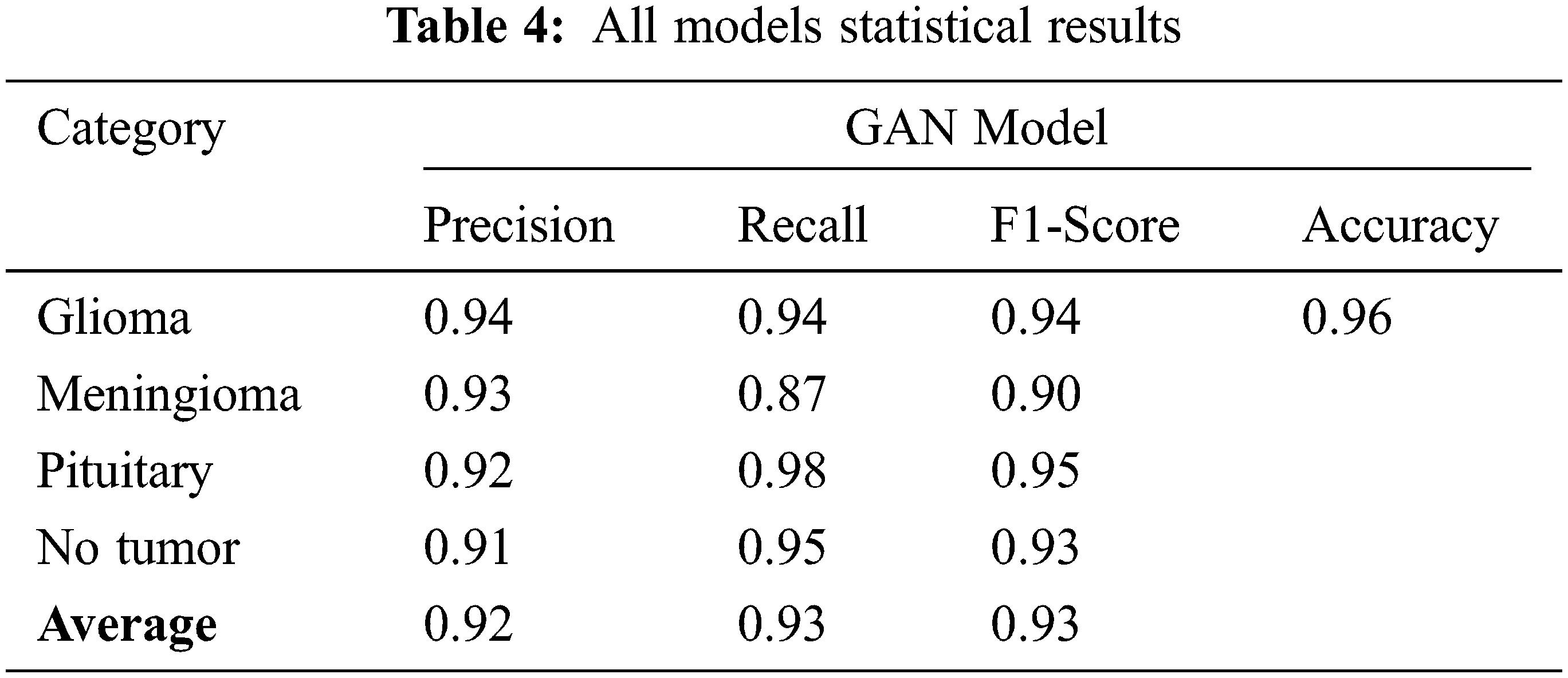
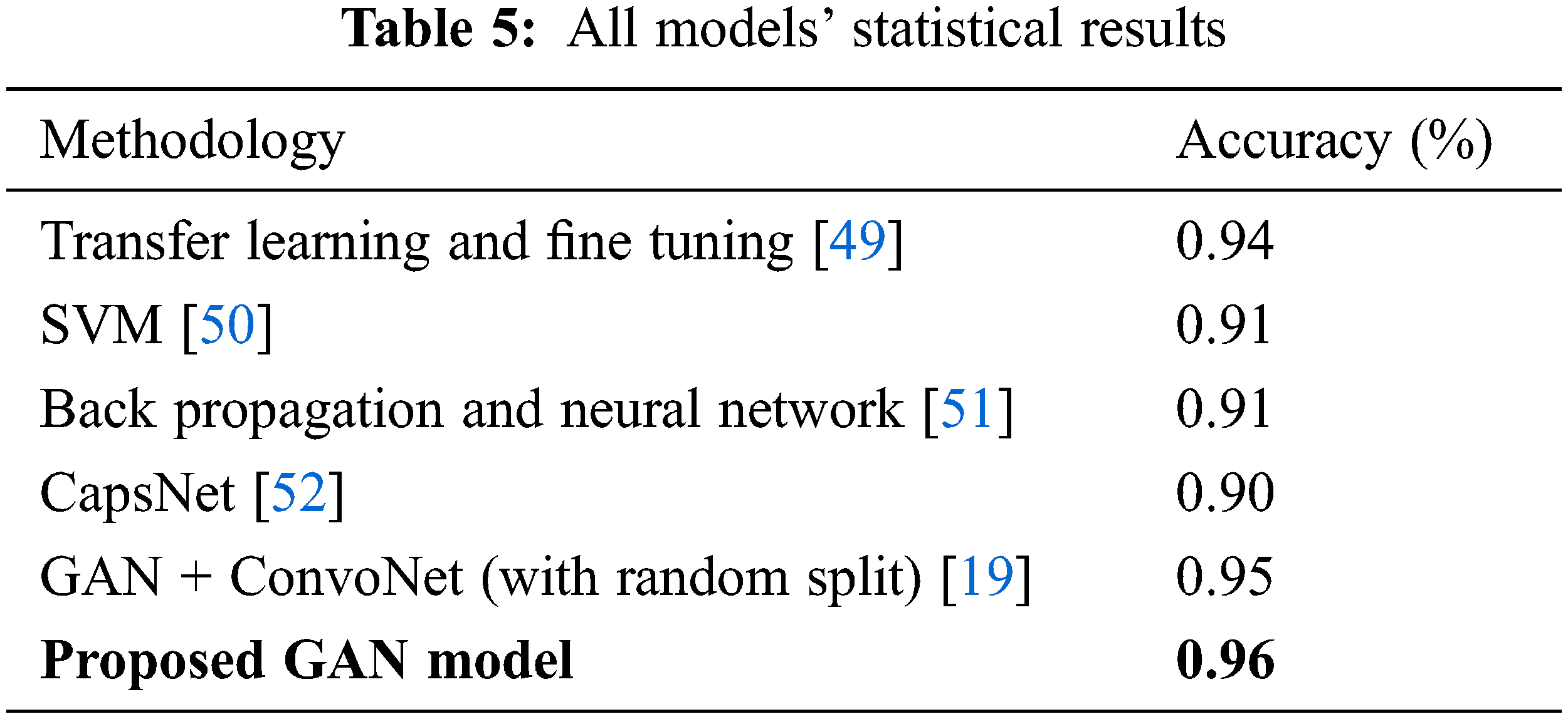
The Tab. 5 compares the accuracy values for all the existing model values. The proposed GAN architecture shows the best accuracy of 0.96% due to its generator and discriminator structures. The other existing approaches show the lowest accuracy. The accuracy value for the GAN proposed model is the highest one as 0.96 shown in Tab. 4.

5  Conclusion

We have proposed a deep learning method known as Generative Adversarial Network (GAN) in this research. It consists of two parts, famous as generator and discriminator. First, a pre-trained CNN model is applied in the discriminator model to extract the robust features and learn the basic structures of MRI images in CNN layers. Then a profound CNN model is applied to differentiate between four tumor classes. The publically available CE-MRI images dataset is used to evaluate the GAN model. It achieved an accuracy of 96%, which is the highest one as compared to the existing techniques. In medical terms, the proposed model would help the generation of real medical image data to maximize the training of the medical experts for the acute prediction of medical diseases.

Funding Statement: Authors would like to acknowledge the support of the Deputy for Research and Innovation-Ministry of Education, Kingdom of Saudi Arabia for funding this research through a project (NU/IFC/ENT/01/014) under the institutional funding committee at Najran University, Kingdom of Saudi Arabia.

Conflicts of Interest: The authors declare that they have no conflicts of interest to report regarding the present study.

References

1. A. S. Lundervold and A. Lundervold, “An overview of deep learning in medical imaging focusing on MRI,” Zeitschrift Für Medizinische Physik, vol. 29, no. 2, pp. 102–127, 2019. [Google Scholar]
2. K. Suzuki, “Overview of deep learning in medical imaging,” Radiological Physics and Technology, vol. 10, no. 3, pp. 257–273, 2017. [Google Scholar]
3. A. Krizhevsky, I. Sutskever and G. E. Hinton, “ImageNet classification with deep convolutional neural networks,” Communications of the ACM, vol. 60, no. 6, pp. 84–90, 2017. [Google Scholar]
4. N. Abiwinanda, M. Hanif, S. T. Hesaputra, A. Handayani and T. R. Mengko, “Brain tumor classification using convolutional neural network,” in Proc. the Int. Federation for Medical and Biological Engineering Proc., Singapore, pp. 183–189, 2019. [Google Scholar]
5. M. L. Goodenberger and R. B. Jenkins, “Genetics of adult glioma,” Cancer Genetics, vol. 205, no. 12, pp. 613–621, 2012. [Google Scholar]
6. A. -R. Fathi and U. Roelcke, “Meningioma,” Current Neurology and Neuroscience Reports, vol. 13, no. 1, pp. 1–8, 2013. [Google Scholar]
7. S. Melmed, “Pituitary-tumor endocrinopathies,” The New England Journal of Medicine, vol. 382, no. 10, pp. 937–950, 2020. [Google Scholar]
8. M. Nazir, S. Shakil and K. Khurshid, “Role of deep learning in brain tumor detection and classification (2015 to 2020A review,” Computerized Medical Imaging and Graphics: The Official Journal of the Computerized Medical Imaging Society, vol. 91, no. 1, pp. 101940–101955, 2021. [Google Scholar]
9. S. Gull and S. Akbar, “Artificial intelligence in brain tumor detection through MRI scans: Advancements and challenges,” in Proc. Artificial Intelligence and Internet of Things Boca Raton, Florida, CRC Press, pp. 241–276, 2021. [Google Scholar]
10. S. Deepak and P. M. Ameer, “Brain tumor classification using deep CNN features via transfer learning,” Computers in Biology and Medicine, vol. 111, no. 1, pp. 103345–103353, 2019. [Google Scholar]
11. Y. Zhou, “Holistic brain tumor screening and classification based on densenet and recurrent neural network,” in Int. MICCAI Brainlesion Workshop. Proc.: Lecture Notes in Computer Science (LNIP, 11383), Milan, Italy, pp. 208–217, 2019. [Google Scholar]
12. X. Yi, E. Walia and P. Babyn, “Generative adversarial network in medical imaging: A review,” Medical Image Analysis, vol. 58, no. 1, pp. 101552–101561, 2019. [Google Scholar]
13. A. Creswell, T. White, V. Dumoulin, K. Arulkumaran, B. Sengupta et al., “Generative adversarial networks: An overview,” IEEE Signal Processing Magazine, vol. 35, no. 1, pp. 53–65, 2018. [Google Scholar]
14. Z. Pan, W. Yu, X. Yi, A. Khan, F. Yuan et al., “Recent progress on generative adversarial networks (GANsA survey,” IEEE Access, vol. 7, no. 1, pp. 36322–36333, 2019. [Google Scholar]
15. L. Rundo, C. Militello, G. Russo, S. Vitabile, M. C. Gilardi et al., “GTVcut for neuro-radiosurgery treatment planning: An MRI brain cancer seeded image segmentation method based on a cellular automata model,” Natural Computing, vol. 17, no. 3, pp. 521–536, 2017. [Google Scholar]
16. J. A. O’reilly, “Automatic segmentation of polycystic kidneys from magnetic resonance images using a three-dimensional fully-convolutional network,” in Proc. 2019 12th Biomedical Engineering Int. Conf., Ubon Ratchathani, Thailand, pp. 1–5, 2020. [Google Scholar]
17. A. Brunetti, L. Carnimeo, G. F. Trotta and V. Bevilacqua, “Computer-assisted frameworks for classification of liver, breast and blood neoplasias via neural networks: A survey based on medical images,” Neurocomputing, vol. 335, no. 12, pp. 274–298, 2019. [Google Scholar]
18. G. Wang, “Automatic brain tumor segmentation using convolutional neural networks with test-time augmentation,” in Proc. Int. MICCAI Brainlesion Workshop, Granada, Spain, pp. 61–72, 2018. [Google Scholar]
19. N. Ghassemi, A. Shoeibi and M. Rouhani, “Deep neural network with generative adversarial networks pre-training for brain tumor classification based on MR images,” Biomedical Signal Processing and Control, vol. 57, no. 1, pp. 101678–101685, 2020. [Google Scholar]
20. J. Liu, Y. Pan, M. Li, Z. Chen, L. Tang et al., “Applications of deep learning to MRI images: A survey,” Big Data Mining and Analytics, vol. 1, no. 1, pp. 1–18, 2018. [Google Scholar]
21. D. N. Louis, A. Perry, G. Reifenberger, A. von Deimling, D. Figarella-Branger et al., “The 2016 world health organization classification of tumors of the central nervous system: A summary,” Acta Neuropathologica, vol. 131, no. 6, pp. 803–820, 2016. [Google Scholar]
22. M. Shibuya, “Pathology and molecular genetics of meningioma: Recent advances,” Neurologia Medico-Chirurgica (Tokyo), vol. 55, no. 1, pp. 14–27, 2015. [Google Scholar]
23. A. E. K. Isselmou, S. Zhang and G. Xu, “A novel approach for brain tumor detection using MRI images,” Journal of Biomedical Science and Engineering, vol. 09, no. 10, pp. 44–52, 2016. [Google Scholar]
24. M. K. Abd-Ellah, A. I. Awad, A. A. M. Khalaf and H. F. A. Hamed, “A review on brain tumor diagnosis from MRI images: Practical implications, key achievements, and lessons learned,” Magnetic Resonance Imaging, vol. 61, no. 1, pp. 300–318, 2019. [Google Scholar]
25. J. C. Kieffer, A. Krol, Z. Jiang, C. C. Chamberlain, E. Scalzetti et al., “Future of laser-based X-ray sources for medical imaging,” Applied Physics B, Lasers and Optics, vol. 74, no. 1, pp. 75–81, 2002. [Google Scholar]
26. Y. E. Almalki1, A. Shaf, T. Ali, M. Aamir, S. K. Alduraibi et al., “Breast cancer detection in Saudi Arabian women using hybrid machine learning on mammographic images,” Computers, Materials & Continua, vol. 72, no. 3, pp. 4833–4851, 2022. [Google Scholar]
27. P. Afshar, A. Mohammadi and K. N. Plataniotis, “Brain tumor type classification via capsule networks,” in Proc. 2018 25th IEEE Int. Conf. on Image Processing (ICIP), Athens, Greece, pp. 3129–3133, 2018. [Google Scholar]
28. I. Goodfellow, “Generative adversarial nets,” in Proc. Advances in Neural Information Processing Systems, Montreal, Quebec, Canada, pp. 2672–2680, 2014. [Google Scholar]
29. A. Radford, L. Metz and S. Chintala, “Unsupervised representation learning with deep convolutional generative adversarial networks,” arXiv: 1511.06434 [cs. LG], 2015. [Google Scholar]
30. I. Goodfellow, “Sherjil 3221 ozair, aaron courville, and yoshua bengio. generative adversarial nets,” arXiv: 1406.2661 [stat. ML], 2014. [Google Scholar]
31. D. Jin, Z. Xu, Y. Tang, A. P. Harrison and D. J. Mollura, “CT-Realistic lung nodule simulation from 3D conditional generative adversarial networks for robust lung segmentation,” in Proc. Medical Image Computing and Computer Assisted Intervention–MICCAI, Granada, Spain, pp. 732–740, 2018. [Google Scholar]
32. W. -C. Hung, Y. -H. Tsai, Y. -T. Liou, Y. -Y. Lin and M. -H. Yang, “Adversarial learning for semi-supervised semantic segmentation,” arXiv: 1802.07934 [cs. CV], 2018. [Google Scholar]
33. F. Milletari, N. Navab and S. -A. Ahmadi, “V-Net: Fully convolutional neural networks for volumetric medical image segmentation,” in Proc. 2016 Fourth Int. Conf. on 3D Vision (3DV), Stanford, CA, USA, pp. 565–571, 2016. [Google Scholar]
34. A. Antoniou, A. Storkey and H. Edwards, “Data augmentation generative adversarial networks,” arXiv: 1711.04340 [stat. ML], 2017. [Google Scholar]
35. G. Mariani, F. Scheidegger, R. Istrate, C. Bekas and C. Malossi, “BAGAN: Data augmentation with balancing GAN,” arXiv: 1803.09655 [cs. CV], 2018. [Google Scholar]
36. S. -W. Huang, C. -T. Lin, S. -P. Chen, Y. -Y. Wu, P. -H. Hsu et al., “AugGAN: Cross domain adaptation with GAN-based data augmentation,” in Proc. Computer Vision–European Conf. on Computer Vision, Munich, Germany, pp. 731–744, 2018. [Google Scholar]
37. X. Ouyang, Y. Cheng, Y. Jiang, C. -L. Li and P. Zhou, “Pedestrian-synthesis-GAN: Generating pedestrian data in real scene and beyond,” arXiv: 1804.02047 [cs. CV], 2018. [Google Scholar]
38. Y. Zhu, “Data augmentation using conditional generative adversarial networks for leaf counting in arabidopsis plants,” in Proc.British Machine Vision Conf., Newcastle, UK, pp. 324–335, 2018. [Google Scholar]
39. P. Costa, A. Galdran, M. I. Meyer, M. Niemeijer, M. Abramoff et al., “End-to-end adversarial retinal image synthesis,” IEEE Transactions on Medical Imaging, vol. 37, no. 3, pp. 781–791, 2018. [Google Scholar]
40. M. J. M. Chuquicusma, S. Hussein, J. Burt and U. Bagci, “How to fool radiologists with generative adversarial networks? A visual turing test for lung cancer diagnosis,” in Proc. 2018 IEEE 15th Int. Symp. on Biomedical Imaging, Washington, DC, USA, pp. 240–244, 2018. [Google Scholar]
41. M. Frid-Adar, I. Diamant, E. Klang, M. Amitai, J. Goldberger et al., “GAN-Based synthetic medical image augmentation for increased CNN performance in liver lesion classification,” Neurocomputing, vol. 321, no. 1, pp. 321–331, 2018. [Google Scholar]
42. C. Han, H. Hayashi, L. Rundo, R. Araki, W. Shimoda et al., “GAN-Based synthetic brain MR image generation,” in Proc. 2018 IEEE 15th Int. Symp. on Biomedical Imaging, Washington, DC, USA, pp. 734–738, 2018. [Google Scholar]
43. H. S. Vu, D. Ueta, K. Hashimoto, K. Maeno, S. Pranata et al., “Anomaly detection with adversarial dual autoencoders,” arXiv: 1902.06924 [cs. CV], 2019. [Google Scholar]
44. P. K. Chahal, S. Pandey and S. Goel, “A survey on brain tumor detection techniques for MR images,” Multimedia Tools and Applications, vol. 79, no. 29–30, pp. 21771–21814, 2020. [Google Scholar]
45. J. Cheng, “Brain tumor dataset,” [Online]. Available: https://figshare.com/articles/dataset/brain_tumor_dataset/1512427, 2022. [Google Scholar]
46. L. von Baumgarten, D. Brucker, A. Tirniceru, Y. Kienast, S. Grau et al., “Bevacizumab has differential and dose-dependent effects on glioma blood vessels and tumor cells,” Clinical Cancer Research: An Official Journal of the American Association for Cancer Research, vol. 17, no. 19, pp. 6192–6205, 2011. [Google Scholar]
47. L. von Baumgarten, D. Brucker, A. Tirniceru, Y. Kienast, S. Grau et al., “Constitutive activation of the EGFR-STAT1 axis increases proliferation of meningioma tumor cells,” Neuro-oncology Advances, vol. 2, no. 1, pp. 8–19, 2020. [Google Scholar]
48. M. Satou, J. Wang, T. Nakano-Tateno, M. Teramachi, T. Suzuki et al., “L-Type amino acid transporter 1, LAT1, in growth hormone-producing pituitary tumor cells,” Molecular and Cellular Endocrinology, vol. 515, no. 1, pp. 110868–110890, 2020. [Google Scholar]
49. Z. N. K. Swati, Q. Zhao, M. Kabir, F. Ali, Z. Ali et al., “Brain tumor classification for MR images using transfer learning and fine-tuning,” Computerized Medical Imaging and Graphics: The Official Journal of the Computerized Medical Imaging Society, vol. 75, no. 1, pp. 34–46, 2019. [Google Scholar]
50. J. Cheng, W. Huang, S. Cao, R. Yang, W. Yang et al., “Enhanced performance of brain tumor classification via tumor region augmentation and partition,” The Public Library of Science One, vol. 10, no. 10, pp. 381–394, 2015. [Google Scholar]
51. M. R. Ismael and I. Abdel-Qader, “Brain tumor classification via statistical features and back-propagation neural network,” in Proc. 2018 IEEE Int. Conf. on Electro/Information Technology (EIT), Rochester, MI, USA, pp. 0252–0257, 2018. [Google Scholar]
52. P. Afshar, K. N. Plataniotis and A. Mohammadi, “Capsule networks for brain tumor classification based on MRI images and coarse tumor boundaries,” in Proc. 2019 IEEE Int. Conf. on Acoustics, Speech and Signal Processing (ICASSP), Brighton, UK, pp. 1368–1372, 2019. [Google Scholar]
Cite This Article
Copyright © 2023 The Author(s). Published by Tech Science Press.
This work is licensed under a Creative Commons Attribution 4.0 International License , which permits unrestricted use, distribution, and reproduction in any medium, provided the original work is properly cited.
Downloads
Citation Tools