Neuro-Based Higher Order Sliding Mode Control for Perturbed Nonlinear Systems

1  Introduction

One of the most challenging problems while dealing with nonlinear systems is uncertainty [1,2]. This uncertainty occurs in system dynamics, system parameter variations and external perturbations [1–3]. The uncertainties may also occur due to un-modeled high frequency dynamics, and neglected nonlinearities in constructing the system mathematical model [4,5]. These uncertainties usually lead to the degraded performance of control systems and sometimes to instability [1–3].

Developing robust controllers for nonlinear systems is a great concern of many researchers over decades especially for real-time control systems [6,7]. A robust controller is the controller which has the ability to function properly even in the existence of uncertainties in system parameters or disturbances. Many methods have been adopted to develop such robust controllers [1,2,6,7]. One of the most popular and effective methods is sliding mode control (SMC) [8,9]. The most powerful advantage of the sliding mode strategy is its ability to work effectively even in the existence of uncertainties and external perturbations. Thus, SMC method is insensitive to changes in system parameters, and perturbations. However, the sliding mode strategy sometimes has chattering which is harmful to the actuators of the control system.

Generally, the design of the SMC controller follows two main steps. The first step is the choice of a sliding surface on which the system trajectory is confined to lie and thus the parameters of this surface will govern the performance of the control system. The second step is to determine an efficient control law that forces the system states to reach the sliding surface from any initial state. In order to assure the system stability, the upper bound of uncertainties must be obtained precisely which cannot be guaranteed. Furthermore, chattering occurs due to the sign function in the overall control.

As a result of the efficiency of SMC in handling uncertainties and nonlinearities of systems, it has been the focus of many researchers over decades. SMC has been successfully applied in many applications. These applications include but are not restricted to space crafts [10,11], time delayed control systems [12,13], and power systems [14,15]. The main power of adopting SMC in these nonlinear systems is its robustness against the structures and unstructured uncertainties and external disturbances that exist in these practical systems. However, the SMC is not without disadvantages. The chattering problem is the main problem of using SMC which may lead to undesirable performance and even instability of the control systems. Thus, many research efforts have been thoroughly seen in the literature trying to achieve the optimal performance of SMC of nonlinear systems [8,16–18].

Recently, many attempts have been seen trying to overcome the chattering problem while using the SMC methodology in nonlinear control systems [19–22]. Many researchers have used the conventional first order sliding mode control techniques with updated control functions [23,24]. They used continuous functions like a sigmoid function instead of the intermittent control function. Nevertheless, using such method affects the robustness of the SMC technique to disturbances as it restricts the system’s trajectories to the vicinity of the sliding surface. Thus, many efforts have thought about higher order SMC techniques that keep the system robustness in the presence of disturbances by forcing the system’s variables and their derivatives to follow the sliding surface [25–28]. Working with higher order SM controllers is very challenging and still open to further developments.

Several second order SMC solutions are developed for nonlinear systems [9,16,18]. Twisting and supertwisting algorithms are among the well-known solutions [16,19,21,27,29]. However, these algorithms are constrained with the necessary knowledge of the time derivative of the sliding variables’ which is unluckily not always available. In order to get adequate controller gains’ values, the time derivative of the sliding variable should be bounded. On the other hand, various adaptive SMC techniques have been developed to adequately tune the controller gains with regards to disturbances [30–32] without considering that s⋅⁡(t) is bounded. Also, using soft computing techniques in developing adaptive SMC approaches for nonlinear systems have been given extensive attention. The main power of using the soft computing techniques comes from their ability to intelligently estimate the system states even for complex systems [33,34]. In [35], the nonlinear terms of the fractional order system are estimated using a radial basis function (RBF) neural network.

It has been apparent that working with higher order SMC is very efficient in overcoming the chattering problem which is the main concern of using SMC in many applications as it may cause high frequency oscillations which leads to actuators damage. However, as the order of SMC increases, the system model turns to be more complex. Developing the adaptive control laws for such complex systems is very challenging. Additionally, the time convergence of these systems cannot be guaranteed. This paper presents a novel adaptive generalized neuro-based SMC for nonlinear systems. The presented approach is of general order which means that we are able to deal with any order of SMC. The developed approach in this paper is supported with strong mathematical analysis and proofs. The main contributions of this work can be summarized as follows:

1.    Developing a neuro-based SMC control approach for nonlinear systems which is capable of completely eliminating the chattering. The proposed approach can be used with any order of sliding mode and thus can be generally used with various types of applications. The neural networks are exploited in the proposed approach for their excellent capabilities in function approximation and thus used to approximate the nonlinearities and uncertainties in the system under consideration. The approximation errors are completely considered in the developed approach. All types of uncertainties have been taken into consideration.

2.    The proposed approach is able to completely and adaptively estimate the uncertainties and thus the problems exist with either estimating the upper bound of the uncertainties (like in [16,19,21,27,29]) or with adaptation of system gains (like in [30–32]) are released.

3.    The stability of the designed system is validated using a suggested quadratic Lyapunov function. The estimated uncertainties are considered in the developed Lyapunov analysis. The developed control law guarantees that the system will reach the sliding surface in finite time with any order of sliding mode. The mathematical proof for the developed approach and the stability analysis are given in details below.

The proposed control algorithm is applied to a position trajectory tracking problem of an inverted pendulum nonlinear system through simulations. The proposed approach is compared to the existing conventional controllers. The simulation results indicate that the control performance of the develoepd control strategy is satisfactory and better than those of the existing conventional controllers.

The remainder of this paper is organized as follows: the problem under consideration is formulated in Section 2. Section 3 presents the proposed higher order sliding mode control for nonlinear systems. The presented adaptive neural network-based higher order sliding mode control is introduced in Section 4. Some simulation results and discussions are presented in Section 5. Finally, conclusions and some future directions are summarized in Section 6.

2  Problem Formulation

The nth order uncertain nonlinear single-input single-output system may be described by:

y(n)(t)=f(x(t),t)+g(x(t),t)u(t)+ρ(t)y(t)=x1(t) (1)

where u(t) is the system input and x(t)=[yy˙y¨.......y(n)y(n−1)]T is the vector of the system states with x1(t)=y(t) . The f(x(t),t) and g(x(t),t) are nonlinear unknown functions. The ρ(t) denotes the external perturbations.

In order to consider uncertainties in the system model, the controlled system can be modified as follows:

y(n)(t)=fn(x(t),t)+Δf(x(t),t)+(gn(x(t),t)+Δg(x(t),t))u(t)+ρ(t)y(n)(t)=fn(x(t),t)+gn(x(t),t)u(t)+δ(t) (2)

where fn(x(t),t) and gn(x(t),t) represent the nominal values of the nonlinear functions f(x(t),t) and g(x(t),t) . Δf(x(t),t) and Δg(x(t),t) represent the parameter variations (uncertainties) of the nonlinear functions f(x(t),t) and g(x(t),t) . All parameters' variations (uncertainties) can be lumped in one variable as follows:

δ(t)=Δf(x(t),t)+Δg(x(t),t)u(t)+ρ(t) (3)

The sliding surface of order r is chosen as:

s(r−1)+αr−2s(r−2)+…+α1s˙+αos=e(n−1)+λn−2e(n−2)+....+λ1e˙+λoe+λI∫e(ξ)dξs(r−1)+∑j=0r−2αjs(j)=e(n−1)+∑i=0n−2λie(i)+λI∫e(ξ)dξ (4)

where e(t)=y(t)−yd(t) is the tracking error, and y(t) , and yd(t) are the actual and desired system responses respectively. The parameters (αo,.....αr−2) , (λo,.....λn−2) and (λI) are positive constants. The addressed problem in this work is to design an adaptive and continuous neuro-based sliding mode control for nonlinear perturbed systems such that the system output y(t) successfully follows a bounded desired signal yd(t) , in the presence of uncertainties. Two models are proposed; discontinuous, and continuous as explained in details below.

3  Higher Order Sliding Mode Control for Higher Order Nonlinear Systems

In this section, a generalized extension of the authors' work in [35] is presented. The developed extended work in this section is based on the design of a discontinuous rth order sliding mode control (DROSMC) for nth order uncertain nonlinear single-input single-output system. In order to achieve that, the trajectory tracking error must approach zero and the ROSMC control law must steer the sliding surface s(t) and all its derivatives ( s(t)=s˙(t)=s¨(t)=.....=s(r−1)(t)=0 ) to zero. To reach this goal, the proposed DROSMC control law is chosen as [15]:

u(t)=ueq(t)+ur(t) (5)

where ueq(t) and ur(t) denote the equivalent control effort and the switching control signal respectively. The equivalent control effort ueq(t) can be obtained as a solution of s(r)(t)=0 under nominal system dynamic model (δ(t)=0) .

The time derivative of sliding surface in Eq. (4) is obtained as:

s(r)+∑j=1r−1αj−1s(j)=e(n)+∑i=1n−1λi−1e(i)+λIe (6)

The rth time derivative of sliding surface is computed as:

s(r)=−∑j=1r−1αj−1s(j)+e(n)+∑i=1n−1λi−1e(i)+λIe (7)

Substituting e(n)(t)=y(n)(t)−yd(n)(t) into Eq. (7) and using Eq. (2), we get:

s(r)=−∑j=1r−1αj−1s(j)+fn+gnu(t)+δ(t)−yd(n)(t)+∑i=1n−1λi−1e(i)+λIe (8)

In order to keep the error variables of the nominal system (δ(t)=0) on the sliding surface, the condition s(r)(t)=0 must be satisfied. Thus, the control signal is recognized as the equivalent control action ueq(t) which can be calculated from Eq. (8) as:

ueq(t)=1gn(∑j=1r−1αj−1s(j)−fn+yd(n)(t)−∑i=1n−1λi−1e(i)−λIe) (9)

The switching control signal ur(t) can be chosen as:

ur(t)=−1gn(kr−1s(r−2)+krsign(s(r−1))+∑i=1r−3ki+1s(i)s(i+1)s(r−1)+ϵ) (10)

where kr is a design parameter representing the reaching control gain, sign(s(r−1)) denotes the signum function, and ϵ is a small positive number.

Theorem 1. Assume the uncertain controlled system (2) is controlled by u(t) (5) which guarantees the global boundedness of all sliding variables and the tracking error approaches zero, the global stability of (2) is verified.

Proof. Consider the following Lyapunov function:

V(t)=k12s2+k22(s˙)2+k32(s¨)2+.......+kr−12(s(r−2))2+12(s(r−1))2V(t)=12∑i=1r−2ki+1(s(i))2+12(s(r−1))2 (11)

where k1,k2,....kr−1 are strict positive constants.

By differentiating V(t), we get:

V˙(t)=k1ss˙+k2s˙s¨+k3s¨s⃛+.......+kr−1s(r−2)s(r−1)+s(r−1)s(r)V˙(t)=∑i=1r−3ki+1s(i)s(i+1)+kr−1s(r−2)s(r−1)+s(r−1)s(r)(12)

Substituting from Eq. (8) into Eq. (12), then:

V˙(t)=∑i=1r−3ki+1s(i)s(i+1)+kr−1s(r−2)s(r−1)+s(r−1){−∑j=1r−1αj−1s(j)+fn+gnu(t)+δ(t)−yd(n)(t)+∑i=1n−1λi−1e(i)+λIe} (13)

Substituting from Eqs. (5) and (9), then:

V˙(t)=∑i=1r−3ki+1s(i)s(i+1)+kr−1s(r−2)s(r−1)+s(r−1){gnur(t)+δ(t)} (14)

Substituting Eq. (10) into Eq. (14):

V˙(t)=∑i=1r−3ki+1s(i)s(i+1)−s(r−1){∑i=1r−3ki+1s(i)s(i+1)s(r−1)+ϵ}−krs(r−1)sign(s(r−1))+s(r−1)δ(t) (15)

By using |s(r−1)|=s(r−1)sign(s(r−1)) and for small positive, Eq. (15) can be rewritten as:

V˙(t)≤−kr|s(r−1)|+s(r−1)δ(t)V˙(t)≤−|s(r−1)|{kr−|δ(t)|} (16)

In order to ensure that the closed loop system is globally stable and the reaching condition V˙(t)<0 is guaranteed, the switching control gain kr must be selected as:

kr>|δ(t)| (17)

End of Proof

The total control law of the developed DROSMC controller can be deduced by substituting from Eqs. (9) and (14) into Eq. (5) as follows:

u(t)=1gn(∑j=1r−1αj−1s(j)−fn+yd(n)(t)−∑i=1n−1λi−1e(i)−λIe−kr−1s(r−2)−krsign(s(r−1))−∑i=1r−3ki+1s(i)s(i+1)s(r−1)+ϵ) (18)

The block diagram of the proposed DROSMC is shown in Fig. 1.

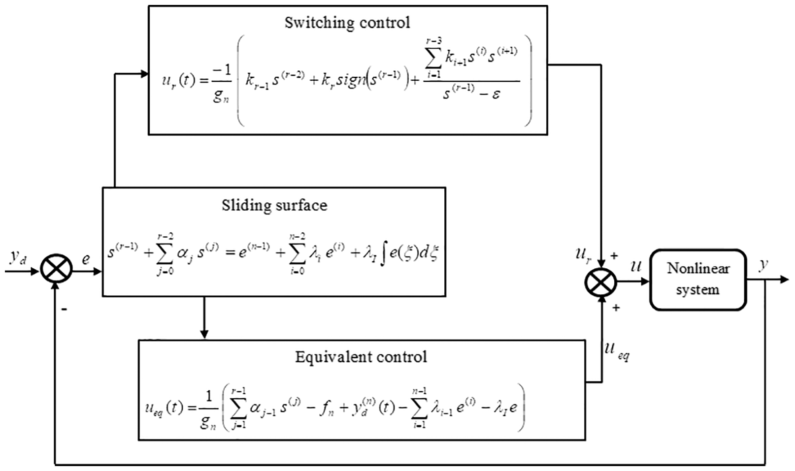
Figure 1: Block diagram of DROSMC

4  Adaptive Neural Network-based Higher Order Sliding Mode Control

Although, the DROSMC controller described in Eq. (18) can ensure the stability of the control system, chattering occurs when using this controller as it contains a discontinuous signum function (krsign(s(r−1))) . Furthermore, the gain Kr is concerned with the boundaries of unknown uncertainties. Thus, it is difficult to implement this controller in practical applications as it requires a precise knowledge of the unknown nonlinear functions (fn) and (gn) . In this section, the radial basis function neural network (RBFNN) is exploited to develop an adaptive RBFNN continuous rth order sliding mode control strategy (ARBFNN-CROSMC). The developed continuous strategy is based on replacing the discontinuous term with a continuous control action. The approximation property of the RBFNN is used to approximate the unknown nonlinear functions (fn) and (gn) as follows:

fn(x(t),t,Wfo)=∑l=1mwfloψl(x)+ϵfo=WfoTΨ(x)+ϵfogn(x(t),t,Wgo)=∑l=1mwgloψl(x)+ϵgo=WgoTΨ(x)+ϵgo (19)

where Wfo=[wf1owf2o......wfmo]T and Wgo=[wg1owg2o......wgmo]T are the optimal output weight vectors of the output layers of the RBFNNs used to approximate the unknown nonlinear functions (fn) and (gn) . ϵfo and ϵgo are the optimal (minimum) estimation errors. Ψ(x)=[ψ1(x)ψ2(x)......ψm(x)]T is m -dimensional vector whose elements denote the Gaussian activation function of hidden layer neurons for each RBFNN and are given by:

ψl(x)=exp⁡(−‖x−cl‖2σl2),l=1,2,3,........m (20)

where cl and σl are the center and width of the lth Gaussian function.

The adaptive RBFNN continuous rth order sliding mode control strategy (ARBFNN-CROSMC) is chosen as:

u(t)=(ueq(t)+ucsmc(t)+uδ(t)) (21)

where ueq(t) is the equivalent control action and is calculated as:

ueq(t)=1g^n(∑j=1r−1αj−1s(j)−f^n+yd(n)(t)−∑i=1n−1λi−1e(i)−λIe) (22)

where f^n and g^n are the approximated nonlinear functions (fn) and (gn) , and are given as:

f^n=∑l=1mw^flψl(x)=W^fTΨ(x)g^n=∑l=1mw^glψl(x)=W^gTΨ(x) (23)

where W^f=[w^f1w^f2......w^fm]T and W^g=[w^g1w^g2......w^gm]T are the m -dimensional adaptive output weight vectors of the linear output layers for the radial basis function neural networks (RBFNNs).

The control signal ucsmc(t) in Eq. (21) is a smooth continuous sliding mode control action that replaces the switching control signal to completely eliminate the chattering amplitude. uδ(t) is an adaptive control term employed to compensate for the unknown uncertainty. The smooth continuous sliding mode control signal ucsmc(t) is chosen as:

ucsmc(t)=−1g^n(kr−1s(r−2)+kr(s(r−1))+∑i=1r−3ki+1s(i)s(i+1)s(r−1)+ϵ) (24)

From Eq. (8), one can have:

s(r)=−∑j=1r−1αj−1s(j)+fn+gnu(t)+δ(t)+g^nu(t)−g^nu(t)−yd(n)(t)+∑i=1n−1λi−1e(i)+λIe (25)

Substituting u(t) from Eq. (21) into Eq. (25) yields:

s(r)=−∑j=1r−1αj−1s(j)+fn+(gnu−g^nu)+δ(t)+g^n(ueq+ucsmc+uδ)−yd(n)(t)+∑i=1n−1λi−1e(i)+λIe (26)

Using Eqs. (22) and (24), Eq. (26) becomes:

s(r)=fn−f^n+(gnu−g^nu)+δ(t)+g^nuδ−kr−1s(r−2)−kr(s(r−1))−∑i=1r−3ki+1s(i)s(i+1)s(r−1)+ϵ (27)

Substituting Eqs. (19) and (23) into Eq. (27) yields:

s(r)=Wf~TΨ(x)+ϵfo+Wg~TΨ(x)u+ϵgou+δ(t)+g^nuδ−kr−1s(r−2)−kr(s(r−1))−∑i=1r−3ki+1s(i)s(i+1)s(r−1)+ϵ (28)

where Wf~=Wfo−Wf^ , Wg~=Wgo−Wg^

Define ς(t) as the total lumped uncertainty that is given as:

ς(t)=ϵfo+ϵgou+δ(t) (29)

Substituting Eq. (29) into Eq. (28) yields:

s(r)=Wf~TΨ(x)+Wg~TΨ(x)u+ς(t)+g^nuδ−kr−1s(r−2)−kr(s(r−1))−∑i=1r−3ki+1s(i)s(i+1)s(r−1)+ϵ (30)

The adaptive control term uδ(t) is chosen as:

uδ(t)=−1g^nς^(t) (31)

where ς^(t) is an adaptive term representing the estimated perturbation that is used to estimate the lumped uncertainty ς(t) in Eq. (29). The global stability of the closed loop system can be proved using the following Lyapunov function:

Theorem 2. Assume the uncertain controlled system (2) is controlled by u(t) (21) which guarantees the global boundedness of all sliding variables and the tracking error approaches zero, the global stability of (2) is verified.

Proof. Consider the following Lyapunov function:

V(t)=12∑i=1r−2ki+1(s(i))2+12(s(r−1))2+12γfWf~TWf~+12γgWg~TWg~+12γςς~2 (32)

where ς~(t) is estimation error of the lumped uncertainty which is defined as:

ς~(t)=ς(t)−ς^(t) (33)

The first derivative of Lyapunov function V˙(t) is:

V˙(t)=∑i=1r−3ki+1s(i)s(i+1)+kr−1s(r−2)s(r−1)+s(r−1)s(r)+γfWf~TWf∼⋅+γgWg~TWg∼⋅+γςς~ς∼⋅ (34)

Substituting from Eq. (30) into Eq. (34):

V˙(t)=∑i=1r−3ki+1s(i)s(i+1)+kr−1s(r−2)s(r−1)+s(r−1){Wf~TΨ(x)+Wg~TΨ(x)u+ς(t)+g^nuδ−kr−1s(r−2)−kr(s(r−1))−∑i=1r−3ki+1s(i)s(i+1)s(r−1)+ϵ}+γfWf~TWf∼⋅+γgWg~TWg∼⋅+γδς~ς∼⋅ (35)

Substituting from Eq. (31) into Eq. (35):

V˙(t)=∑i=1r−3ki+1s(i)s(i+1)−kr(s(r−1))2−s(r−1)∑i=1r−3ki+1s(i)s(i+1)s(r−1)+ϵ+s(r−1){Wf~TΨ(x)+Wg~TΨ(x)u+ς~(t)}+γfWf~TWf∼⋅+γgWg~TWg∼⋅+γδς~ς∼⋅ (36)

Rearranging Eq. (36) results in:

V˙(t)=∑i=1r−3ki+1s(i)s(i+1)−kr(s(r−1)−s(r−1)∑i=1r−3ki+1s(i)s(i+1)s(r−1)+ϵ+Wf~T(s(r−1)φ(x)−γfWf∧⋅)+Wg~T(s(r−1)φ(x)u−γgWg∧⋅)+ς~(t)(s(r−1)−γδς∧⋅) (37)

In order to ensure that the closed loop system is globally stable and the reaching condition V˙(t)<0 is guaranteed, the adaptive output weight vectors of the linear output layers for the radial basis function neural networks (RBFNNs) must be selected as:

Wf∧⋅=1γfs(r−1)φ(x)Wg∧⋅=1γgs(r−1)φ(x)u (38)

The time evolution of the estimated uncertainty ς^ can be chosen as:

ς∧⋅=1γδs(r−1) (39)

Substituting Eqs. (38) and (39) into Eq. (37) yields:

V˙(t)=∑i=1r−3ki+1s(i)s(i+1)−kr(s(r−1))2−s(r−1)∑i=1r−3ki+1s(i)s(i+1)s(r−1)+ϵ (40)

For a small positive number ϵ , Eq. (40) can be rewritten as:

V˙(t)≤−kr(s(r−1))2 (41)

From the above analysis, the global asymptotic stability of the closed loop system is guaranteed.

End of Proof

5  Simulation Results

In order to validate the effectiveness of the proposed ARBFNN-CROSMC control methodology, the stabilization control of the inverted pendulum (IP) system [36,37] is implemented in this section.

5.1 Second Order Sliding Mode Control

First, a discontinuous second order sliding mode control approach (D2SMC) and an adaptive RBFNN continuous second order sliding mode control strategy (ARBFNN-C2SMC) are implemented using the inverted pendulum system. The performance of both conventional PID controller and D2SMC are compared to demonstrate the efficacy of the proposed ARBFNN-C2SMC control strategy. Two main problems are implemented; the set point tracking control problem, and the trajectory tracking control problem.

5.1.1 Set Point Tracking Control Problem

To check the ability of the proposed strategy to reach a desired reference point, a desired angular position is set at θd=0 . A step disturbance force 5000 N is suddenly applied at t=2.5 s to clarify the robustness of the proposed ARBFNN-C2SMC control scheme in the presence of uncertainties. The standalone PID parameters are set as: kp=100 , ki=10 and kd=100 . The parameters of the D2SMC are set as: αo=0.6 , λo=1.2 , λI=1 , k1=2.5 and k2=150 . The parameters of the proposed ARBFNN-C2SMC are set as: αo=0.5 , λo=1.25 , λI=1 , γf=0.8 , γg=0.75 , γδ=1 , k1=100 and k2=150 . Fig. 2 shows the angular position response.

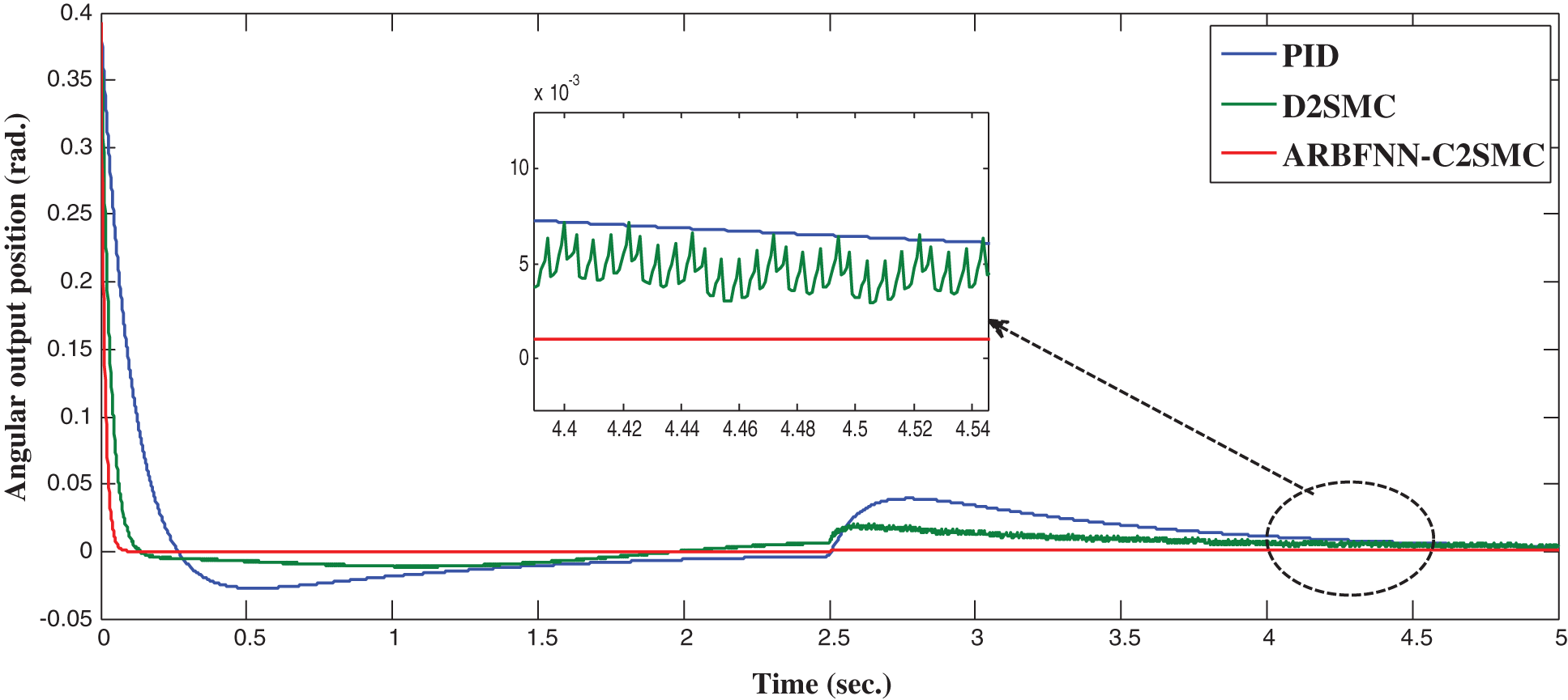
Figure 2: Angular position response in set-point control

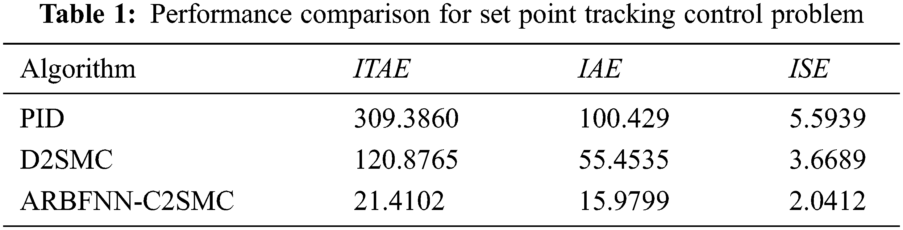
Fig. 2 shows the superiority of the proposed ARBFNN-C2SMC for set point tracking control compared with other approaches even in the presence of external disturbance. In order to assess more the performance of the proposed approach, a comparison of the performance of the proposed approach is compared with other approaches using three performance indices; integral absolute error (IAE), integral time multiplied absolute error (ITAE) and integral of squared error (ISE) which are given by [9]:

IAE=∫|e(t)|dtITAE=∫t|e(t)|dtISE=∫e2(t)dt (42)

Tab. 1 summarizes the results of the performance comparison.

5.1.2 Trajectory Tracking Control Problem

In this subsection, the performance of the proposed approach is assessed in case of trajectory tracking control problem. The standalone PID parameters are set as: kp=150 , ki=75 and kd=140 . The parameters of the D2SMC are set as: αo=1.2 , λo=1.5 , λI=1 , k1=3.2 and k2=175 . The parameters of the proposed ARBFNN-C2SMC are set as: αo=1 , λo=1.1 , λI=1 , γf=1.2 , γg=1.1 , γδ=1 , k1=150 and k2=200 . A step disturbance force of 1000 N is suddenly applied at the pole at t = 5 s to check the robustness of the developed approach in the presence of uncertainties. Fig. 3 shows the system response profile. Fig. 4 illustrates the position error.

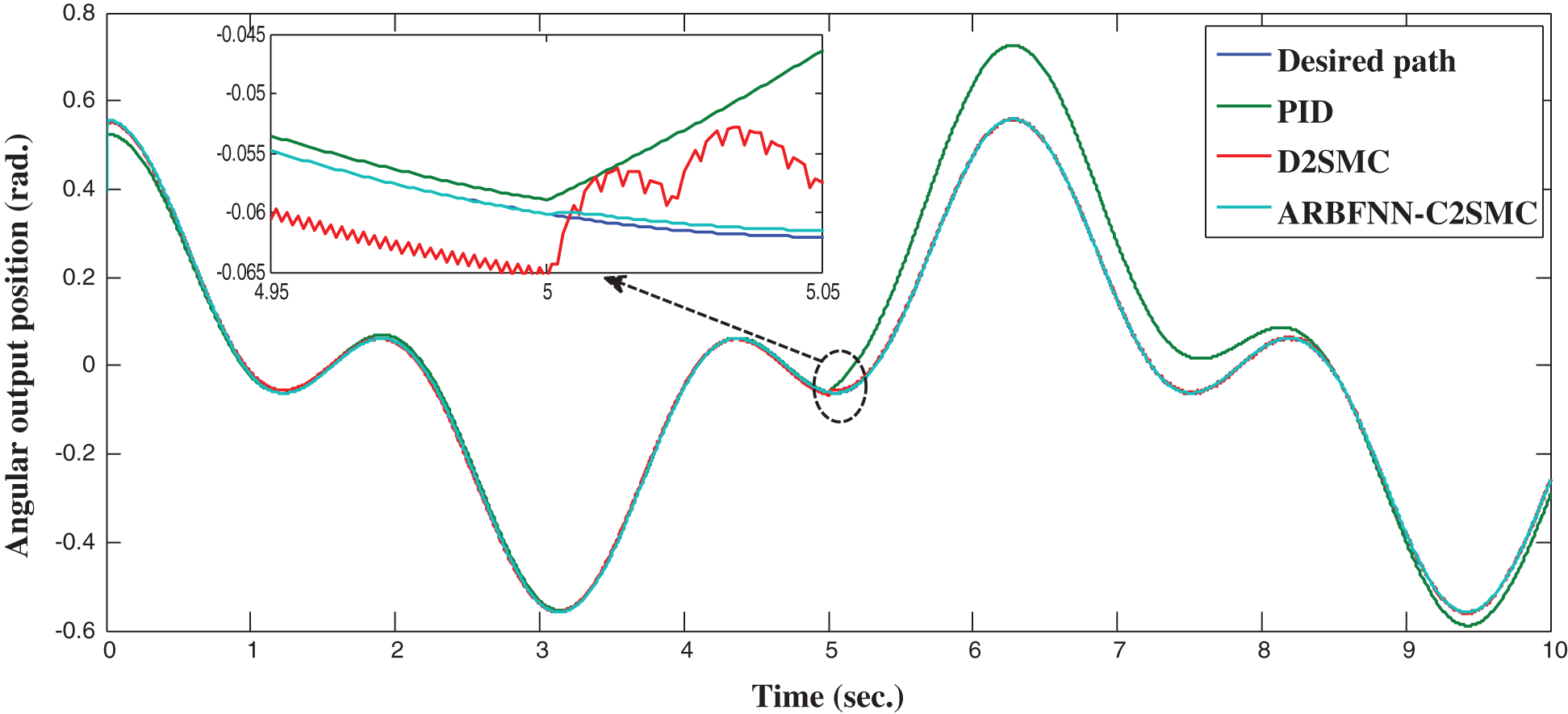
Figure 3: Angular position response in trajectory tracking

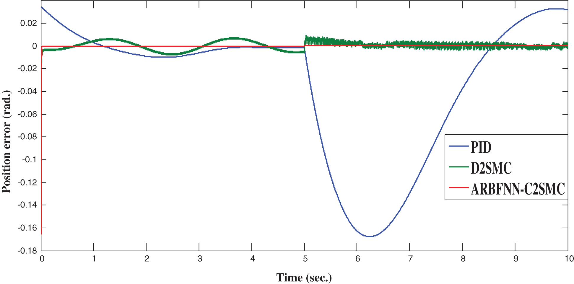
Figure 4: Position error for trajectory tracking control

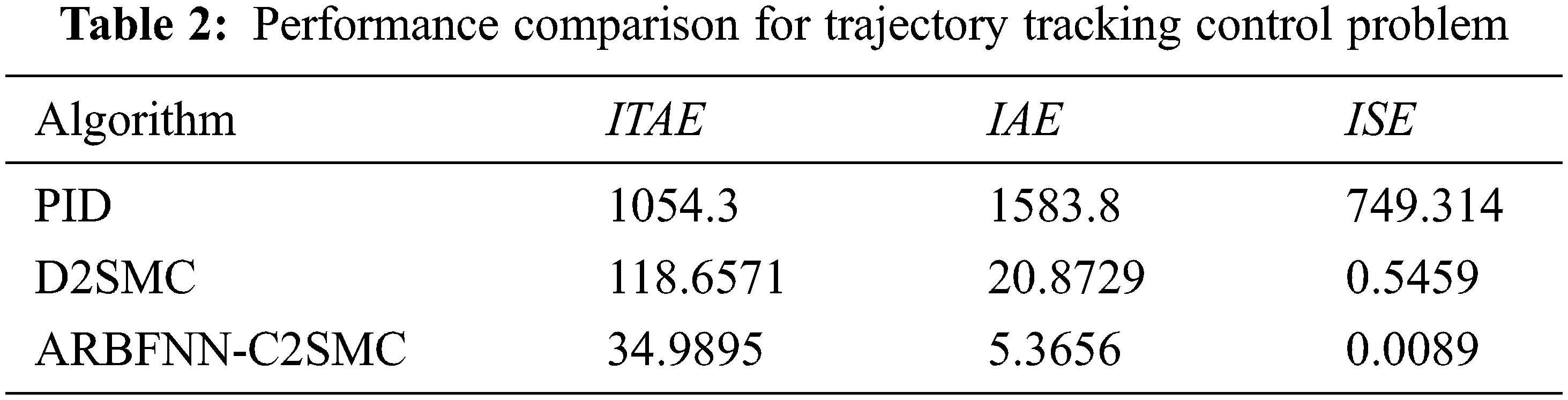
Again, the simulation results illustrate the superiority of the proposed control approach compared with other approaches in case of trajectory tracking control problem. As seen, the D2SMC controller has severe chattering while the proposed approach is able to completely eliminate any type of chattering. A comparison of tracking response characteristics are summarized in Tab. 2 which shows the efficiency of the proposed approach compared with other approaches.

5.2 Third Order Sliding Mode Control

Second, the performance of the proposed approach is assessed in case of using third order sliding mode control (r = 3). Thus, the performance of the proposed adaptive RBFNN continuous third order sliding mode control strategy (ARBFNN-C3SMC) is compared with a discontinuous third order sliding mode control approach (D3SMC), and conventional PID controller.

5.2.1 Set Point Tracking Control Problem

The reference desired angular position is set as: θd=0 . In order to clarify robustness of the proposed ARBFNN-C3SMC control scheme, a step disturbance force of 5000 N is suddenly applied at t = 2.5 sec. The standalone PID parameters are set as: kp=100 , ki=10 and kd=100 . The parameters of the D3SMC are set as: αo=1 , α1=1.2 , λo=1.4 , λI=1 , k2=2.5 and k3=175 . The parameters of the proposed ARBFNN-C3SMC are set as: αo=1 , α1=1 , λo=1 , λI=1 , γf=1 , γg=1 , γδ=1 , k2=120 and k3=250 . Fig. 6 shows the angular position (θ) response profile.

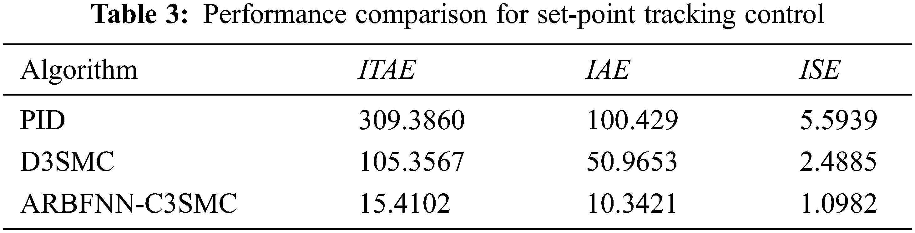
As seen in Fig. 5, the performance of the proposed ARBFNN-C3SMC approach is superior compared with other approaches even in the presence of uncertainties. The proposed approach is able to completely eliminate chattering which other approaches suffer from. A comparison of tracking response characteristics are summarized in Tab. 3 which shows the efficiency of the proposed approach compared with other approaches.

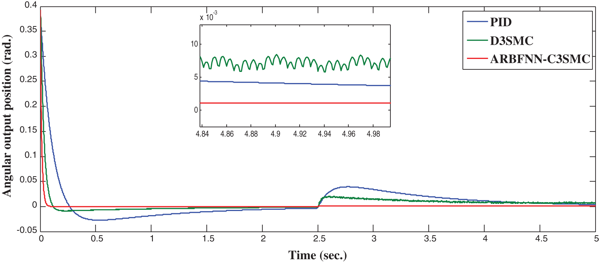
Figure 5: Angular position response in set-point control

5.2.2 Trajectory Tracking Control Problem

In this subsection, the performance of the proposed approach is assessed in case of trajectory tracking control problem. A step disturbance force of 1000 N is suddenly applied at the pole at t = 5 sec to check the robustness of the developed approach in the presence of uncertainties. Fig. 6 shows the system response profile. Fig. 7 illustrates the position error.

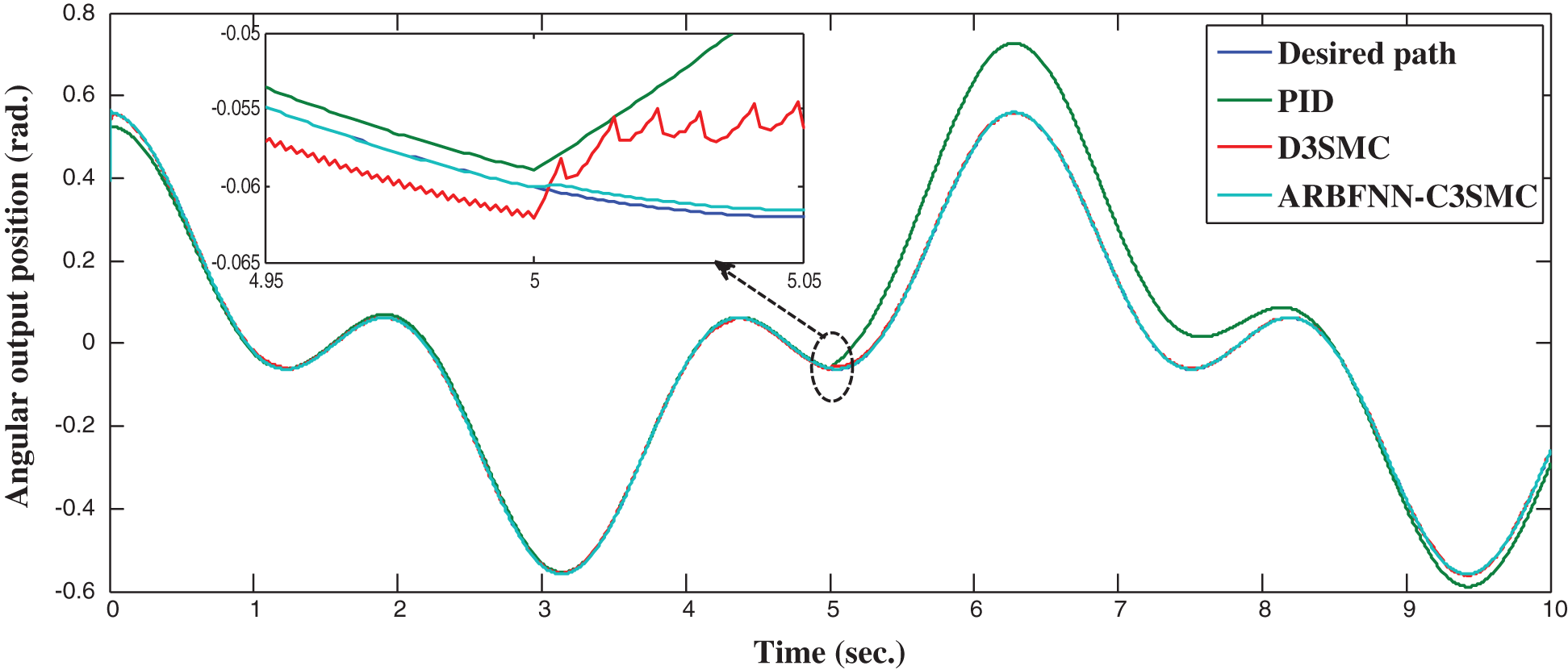
Figure 6: Angular position response in trajectory tracking

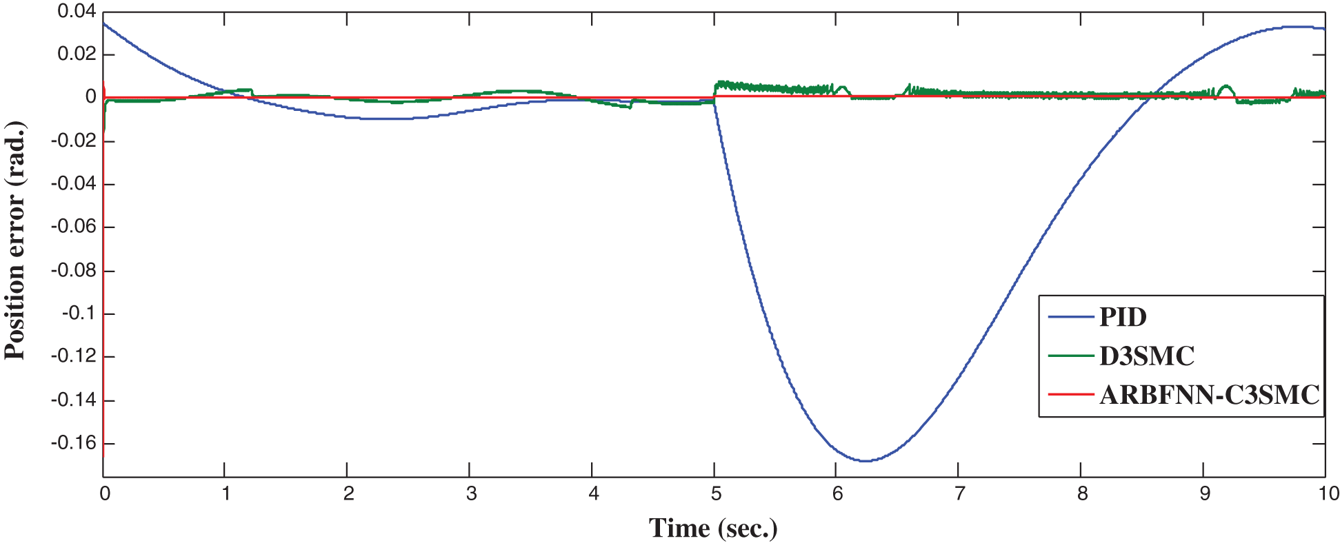
Figure 7: Position error for trajectory tracking control

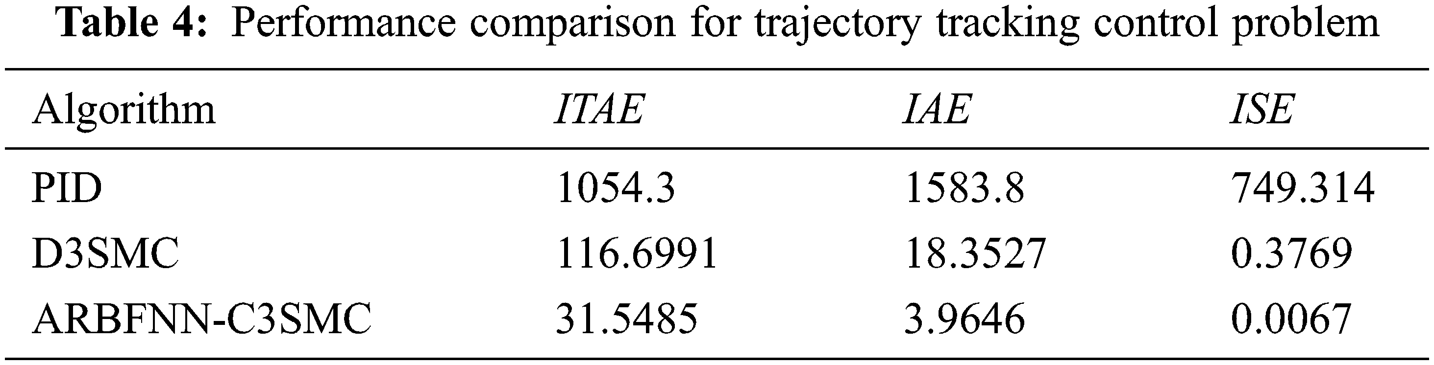
Again, the simulation results illustrate the superiority of the proposed control approach compared with other approaches in case of trajectory tracking control problem. As seen, the D3SMC controller has severe chattering while the proposed approach is able to completely eliminate any type of chattering. A comparison of tracking response characteristics are summarized in Tab. 4 which shows the efficiency of the proposed approach compared with other approaches.

6  Conclusions

An adaptive radial basis function neural network-based generalized rth order sliding mode control approach for nth order uncertain nonlinear systems is developed in this paper. The proposed approach is able to deal with severe uncertainties even for high order nonlinear systems. The proposed approach employed the radial basis function neural networks for their efficiency in approximating nonlinear functions. The proposed approach has been validated theoretically for generalized rth order sliding mode control. The simulation results showed that the proposed approach has great performance compared with other approaches.

Acknowledgement: The authors extend their appreciation to the Deputyship for Research & Innovation, Ministry of Education in Saudi Arabia for funding this research work through the project number (IF-PSAU-2021/01/17796).

Funding Statement: This work is funded by the Deputyship for Research & Innovation, Ministry of Education in Saudi Arabia through the project number (IF-PSAU-2021/01/17796).

Conflicts of Interest: The authors declare that they have no conflicts of interest to report regarding the present study.

References

 1.  R. López, E. Tec-Caamal and M. González, “Observer-based control for uncertain nonlinear systems applied to continuous biochemical reactors,” Mathematical Problems in Engineering, vol. 2020, no. 1, pp. 1–8, 2020. [Google Scholar]

 2.  A. Perrusquía and W. Yu, “Robust control under worst-case uncertainty for unknown nonlinear systems using modified reinforcement learning,” International Journal of Robust and Nonlinear Control, vol. 30, no. 7, pp. 2920–2936, 2020. [Google Scholar]

 3.  D. Vrabie and F. Lewis, “Neural network approach to continuous time direct adaptive optimal control for partially unknown nonlinear systems,” Neural Network, vol. 22, no. 3, pp. 237–246, 2009. [Google Scholar]

 4.  J. Chen, J. Wang and W. Wang, “Robust adaptive control for nonlinear aircraft system with uncertainties,” Applied Sciences, vol. 10, no. 12, pp. 1–16, 2020. [Google Scholar]

 5.  S. Pramod, S. Prasheel and B. Patre, “Robust sliding mode control for systems with noise and unmodeled dynamics based on uncertainty and disturbance estimation (UDE),” International Journal of Computer Applications, vol. 1, no. 9, pp. 37–42, 2010. [Google Scholar]

 6.  P. Khlaeoom and T. Rugthum, “Robust control of uncertain nonlinear systems using neural networks,” in 2019 16th Int. Conf. on Electrical Engineering/Electronics, Computer Telecommunications and Information Technology (ECTI-CON), Pattaya, Thailand, pp. 167–170, 2019. [Google Scholar]

 7.  X. Li, J. Cao and D. Ho, “Impulsive control of nonlinear systems with time-varying delay and applications,” IEEE Transactions on Cybernetics, vol. 50, no. 6, pp. 2661–2673, 2020. [Google Scholar]

 8.  J. Jiang, H. Li, K. Zhao, D. Cao and J. Guirao, “Finite time stability and sliding mode control for uncertain variable fractional order nonlinear systems,” Advances in Differrential Equation, vol. 2021, no. 127, pp. 1–16, 2021. [Google Scholar]

 9.  W. Elawady, Y. Bouteraa and A. Elmogy, “An adaptive second order sliding mode inverse kinematics approach for serial kinematic chain robot manipulators,” Robotics. MDPI, vol. 9, no. 1, pp. 1–26, 2020. [Google Scholar]

10. X. Zhu, J. Chen and Z. Zhu, “Adaptive sliding mode disturbance observer-based control for rendezvous with non-cooperative spacecraft,” Acta Astronautica, vol. 183, no. 5, pp. 59–74, 2021. [Google Scholar]

11. Y. Huang, M. Zhu, L. Sun, Z. Zheng and C. Jin, “Adaptive backstepping control for autonomous shipboard landing of a quadrotor with input saturation,” Asian Journal of Control, vol. 23, no. 4, pp. 1693–1706, 2021. [Google Scholar]

12. Y. Roh and J. Oh, “Robust stabilization of uncertain input-delay systems by sliding mode control with delay compensation,” Automatica, vol. 35, no. 11, pp. 1681–1685, 1999. [Google Scholar]

13. K. Kumari and S. Janardhanan, “Sliding mode control of uncertain time delay system using Lambert W function,” IFAC, vol. 49, no. 1, pp. 173–177, 2016. [Google Scholar]

14. H. ElFadil, M. Oulcaid, A. Yahya, L. Ammeh and F. Giri, “Adaptive sliding mode control of power system with photovoltaic generator,” in 2019 16th Int. Multi-Conf. on Systems, Signals & Devices (SSD), Istanbul, Turkey, pp. 213–218, 2019. [Google Scholar]

15. A. Muthana and Z. Mohamed, “Sliding mode control of chaos in a single machine connected to an infinite bus power system,” Mathematical Problems in Engineering, vol. 2018, no. 1, pp. 1–13, 2018. [Google Scholar]

16. N. Liu, R. Ling, Q. Huang and Z. Zhu, “Second-order super-twisting sliding mode control for finite-time leader-follower consensus with uncertain nonlinear multiagent systems,” Mathematical Problems in Engineering, vol. 2015, no. 8, pp. 1–8, 2015. [Google Scholar]

17. J. Chang, “Optimal sliding mode controller for a class of cascade uncertain nonlinear system,” Journal of Jishou University (Natural Science Edition), vol. 24, no. 3, pp. 13–18, 2003. [Google Scholar]

18. H. Pang and L. Wang, “Global robust optimal sliding mode control for a class of affine nonlinear systems with uncertainties based on SDRE,” in 2009 Second Int. Workshop on Computer Science and Engineering, Qingdao, China, pp. 276–280, 2009. [Google Scholar]

19. T. Gonzalez, J. Moreno and T. Fridman, “Variable gain super-twisting sliding mode control,” IEEE Trans. Automat. Contr., vol. 57, no. 20, pp. 2100–2105, 2012. [Google Scholar]

20. J. Chang, “On chattering-free dynamic dliding mode controller design,” Journal of Control Science and Engineering, vol. 2012, no. 1, pp. 1–7, 2012. [Google Scholar]

21. B. Belabbas, T. Allaoui, M. Tadjine, M. Denai and U. Hatfield, “Higher performance of the super-twisting sliding mode controller for indirect power control of wind generator based on a doubly fed induction generator,” in 2017 5th Int. Conf. on Electrical Engineering (ICEE-B), Boumerdes, Algeria, pp. 1–6, 2017. [Google Scholar]

22. J. Fang, J. Tsai, J. Yan and S. Guo, “Adaptive chattering-free sliding mode control of chaotic systems with unknown input nonlinearity via smooth hyperbolic tangent function,” Mathematical Problems in Engineering, vol. 2019, no. 1, pp. 1–9, 2019. [Google Scholar]

23. H. Elmali and N. Olgac, “Sliding mode control with perturbation estimation (SMCPEA new approach,” International Journal of Control, vol. 56, no. 4, pp. 923–941, 1992. [Google Scholar]

24. J. Burton and A. Zinober, “Continuous approximation of variable structure control,” International Journal of Systems Science, vol. 17, no. 6, pp. 875–885, 1986. [Google Scholar]

25. A. Levant, “Higher-order sliding modes, differentiation and output-feedback control,” International Journal of Control, vol. 76, no. 9–10, pp. 924–941, 2003. [Google Scholar]

26. J. Liu, Y. Zhao, B. Geng and B. Xiao, “Adaptive second order sliding mode control of a fuel cell hybrid system for electric vehicle applications,” Mathematical Problems in Engineering, vol. 2015, no. 1, pp. 1–14, 2015. [Google Scholar]

27. V. Utkin and A. Poznyak, “Adaptive sliding mode control with application to super-twist algorithm: Equivalent control method,” Automatica, vol. 49, no. 1, pp. 39–47, 2013. [Google Scholar]

28. Y. Shtessel, M. Taleb and F. Plestan, “A novel adaptive-gain supertwisting sliding mode controller: Methodology and application,” Automatica, vol. 48, no. 5, pp. 759–769, 2012. [Google Scholar]

29. J. Yang, S. Li and X. Yu, “Sliding-mode control for systems with mismatched uncertainties via a disturbance observer,” IEEE Transactions on Industrial Electronics, vol. 60, no. 1, pp. 160–169, 2016. [Google Scholar]

30. J. Guo, Y. Liu, C. Cheng and J. Zhou, “Disturbance attenuation-based sliding mode control with disturbance observer for mismatched uncertain system,” Advances in Mechanical Engineering, vol. 9, no. 8, pp. 1–11, 2017. [Google Scholar]

31. J. Baek and W. Kwon, “Practical adaptive sliding-mode control approach for precise tracking of robot manipulators,” Journal of Applied Sciences, MDPI, vol. 10, no. 8, pp. 1–16, 2020. [Google Scholar]

32. V. Venkataiah, R. Mohanty and M. Nagaratna, “Review on intelligent and soft computing techniques to predict software cost estimation,” International Journal of Applied Engineering Research, vol. 12, no. 22, pp. 12665–12681, 2017. [Google Scholar]

33. V. Bevilacqua, E. Grasso, G. Mastronardi and L. Riccardi, “A soft computing approach to the intelligent control,” in 2006 4th IEEE Int. Conf. on Industrial Informatics, Singapore, pp. 1312–1317, 2006. [Google Scholar]

34. X. Zhang and W. Huang, “Adaptive neural network sliding mode control for nonlinear singular fractional order systems with mismatched uncertainties,” Fractal and Fractional, vol. 4, no. 50, pp. 1–13, 2020. [Google Scholar]

35. N. Moawad, W. Elawady and A. Sarhan, “Development of an adaptive radial basis function neural network estimator-based continuous sliding mode control for uncertain nonlinear systems,” ISA Transactions, vol. 87, no. 8, pp. 200–216, 2018. [Google Scholar]

36. M. Mohamed, M. Abdallah and A. Mahmoud, “Modeling of inverted pendulum system with gravitational search algorithm optimized controller,” Ain Shams Engineering Journal, vol. 10, no. 1, pp. 129–149, 2019. [Google Scholar]

37. P. Strakoš and J. Tůma, “Mathematical modelling and controller design of inverted pendulum,” in 2017 18th Int. Carpathian Control Conf. (ICCC), Sinaia, Romania, pp. 388–393, 2017. [Google Scholar]