Activation Functions Effect on Fractal Coding Using Neural Networks

1  Introduction

The systems of iterated functions (IFSs) are used to construct fractals. The result of this construction is always self-similar. A fractal is a figure formed by the union of several copies of itself [1–3], where each copy is obtained through a function as part of a system of recursive functions. The functions of this system are usually retractable, and thus they closely group the points and make the shapes shrink down to become part of the overall shape. The fractal shape generated by this system of functions consists of several overlapping small copies of itself. This process is repeated ad infinitum. Each fractal consists of copies of itself, with self-similarity being the most important characteristic of the fractal shapes. The inverse operation is called fractal image coding. The code of the IFS is constructed through this process to generate a fractal image. Identifying the function code is one of the most important challenges in artificial neural networks. A neural network has several activation functions, and the proper selection of these functions is important in fractal coding. With a nonsingular and nonlocal kernel, the overall depiction of HIV infection was highlighted by Tang et al. [4] using the Atangana Baleanu (AB) fractional operator. Considering an artificial neural network devised for the purpose of solving the fractal inverse problem, Al-Jawfi examined the impact of varying the learning rate value in such a system [5]. Fractal Image Compression is the most common application for solving the inverse problem of fractals [6].

2  Backpropagation and IFS

To understand fractal coding with activation functions, we summarize the related existing knowledge in this section.

A loop-free network with its units in a layered arrangement is known as a multilayer (feed-forward) perceptron (MLP), where it is trained via the backpropagation algorithm. After processing in each layer, the inputs of each unit are the outputs of the previous unit in the artificial neural network. As fixed input units, the bias units are included in the first layer. It is possible to form trainable “hidden units” that have internal representations on several layers, as well as a trainable output unit on another layer [7,8]. In some ranges like the interval [0, 1], both the output and input are continuous values; therefore, every unit should be non-binary. The sigmoidal function is the output of a weighted sum. Therefore, the output xi is xi=fi(∑⁡wikxk) , whereby fi represents a sigmoidal function:

fi(t)=11+e−(αt). (1)

The input is xk and the corresponding weights are wik .

The logistic growth rate, which is also called the curve’s steepness in some cases, is represented by the constant α. By considering the neural network environment’s components, the evaluation of the output units is carried out. The network is fed with a set of training patterns as input patterns p and the output units are the corresponding desired target patterns tp . The input p elicits the target output pattern Op , whose purpose is error minimization by adjusting the network’s weights [9].

E=∑p⁡∑k⁡(tkp−okp)2 (2)

This evaluation’s gradation to an input from a unit bias can be determined from the multiplication formula developed by Rumelhart et al. [10]. This process can be extended using the backpropagation method over the whole network.

Numerous lower bounds that are false can be avoided through this scheme. The corresponding fi(x)=(tkp−okp)2 is considered and the input pattern p is fixed for each input cycle.

In this equation, the set of k ranges above the mapped output units. There are various interconnected units in the network, where the interconnection is dependent on the weights wij . For the reduction of error E, stepwise descent is used in varying the weights wij , which is the aim of the learning rule:

Δwij=−∂E∂wij=2∑k⁡(tk−ok)∂ok∂wij. (3)

The exceedingly low growth rate results in the extremely slow network learning in standard backpropagation [11,12]. The objective function differs from the weights due to the high growth rate in the activation functions. Therefore, there is no occurrence of learning. As in linear models, Hess matrix [13] can be utilized to calculate acceptable growth rates, provided that the activation function is quadratic. Furthermore, if there are numerous global and local options in the activation function, the ideal growth rate varies quickly in the training process since the Hessian matrix varies quickly, as in the hidden units in a typical neural network. Trial and error are a tedious process that is usually a requirement in training a neural network that has a fixed growth rate, as in a typical neural network.

A theoretical defect similar to that of standard backpropagation has been observed for different backpropagation types that have been designed. The slope of the gradient should not be an input to the function representing the change in the weights’ magnitude.

Small arbitrary network initialization weights result in a big step size being needed and small gradient in some weight workspace areas. In addition, the network being near to the local minimum will also lead to small step size and gradient in other workspace areas. Similarly, a large or small step size may be required for large gradient value. The algorithms’ tendency for growth rate adaptation is one of the artificial neural networks’ most significant features. Nevertheless, if there are abrupt changes, the calculation of the resultant change of the network weights’ value will be done with the gradient’s growth rate being doubled by the algorithm. Unstable behavior can result from this process occasionally. For obtaining good step sizes, gradients as well as second-order derivatives are utilized in traditional optimization algorithms.

Through further training, it is difficult to construct an algorithm with automatic growth rate adjustment during training. Many of the proposed recommendations in existing studies do not work.

Considering some of these proposals, LeCun et al. [14] and Leen et al. [15] highlighted some encouraging outcomes; however, problems were illustrated but no solution was proposed by them. Rather than varying the growth rate, the weights were adjusted instead by Darken et al. [16]. By maintaining the running weight’s average values, theoretical and ideal convergence rates can be achieved through “polyac averaging” or “iterate averaging” [17,18], which represent a different stochastic approximation type.

In general, S=∪iNfi(s) , where S⊆Rnandfi:Rn→Rn are the functions that require iteration, with

fi(x)=(bi11bi12bi21bi22)(xy)+(bi13bi23). (4)

The union of functions fi is known as the Hutchinson operator fixed point and is represented as S.

2.1 Properties of IFSs

A monoid with composition operation is formed by the collection of functions fi . If two functions are involved, the monoid is called dyadic. An infinite binary tree is considered to represent the composition, where at each tree node, it can be composed of right or left branch. Generally, the composition may be visualized as a p-adic tree, where the number of functions is p.

Which function will be involved in the composition is indicated by each p-adic number’s digit, hence implying that there is isomorphism between the p-adic numbers and the monoid elements [19].

The modular group is part of the dyadic monoid’s automorphism group. For many fractals, including the de Rham curves as well as Cantor set, this group can explain the fractal self-similarity. A matrix can be used to represent the functions, which should be affine transformations, in unique cases. Nevertheless, projective transformations and Möbius transformations are non-linear functions that can be used to build the systems of iterated function. The fractal flame represents one example of a system of iterated functions that has nonlinear functions. To compute the IFS of fractals, the most popular algorithm used is the chaos game. For this algorithm, a point is arbitrarily selected in the fractal space; next, the system of iterated functions is randomly selected, where it is subsequently drawn and applied on the point.

For the plotting of the aftereffects of the application of each capacities group until an initial shape or point is achieved, every possible succession of capacities is obtained until the largest extent of length in the elective calculation process.

The identification of every feasible sequence of functions until a particular maximum length and the plotting of the application result for the sequence of functions until an inittial shape or point is achieved are the alternative algorithm’s most vital goal.

2.2 IFS Rendering

The setting of the attractor is as in [2,16] for a particular set in Rn when building an effective IFS. It may not be possible to solve this inverse problem due to its difficulty [20]. Nevertheless, if self-similarity exists for the given set, these functions’ required construction will be simple. Utilizing the property of self-similarity, mathematical transformations can be carried out to obtain the system of iterated functions.

On the probability measures’ space P(C), the contraction mapping’s fixed point is known as the fractal shape [21].

2.3 Using Neural Networks to Code IFS

These fixed points of the network architecture are used in the representation of elements in the Hopfield network. The encoding of fractional attraction by an IFS represents the network dynamics, where examples of network dynamics utilization are the research by Giles et al. [8] and Melnik [11], who studied positional activation in networks. For a random number of times, one of the transformations of the system was applied to a selected point by Melnik [11] and Barnsley et al. [2] until convergence to the attractor occurred.

For a particular fractal attractor, a set of weights corresponding to the neural network can be identified for the purpose of attractor approximation. For this research, XoutandYout are the output units while Xin and Yin are the input units of the neural network with six weights per transformation (IFS); together, they are a representation of a function that has a homogeneous recursive function system state (Fig. 1). For other IFS cases, the number of weights, outputs, and inputs may be different. Random selection is used with regard to the choice of transformation. For every fractal image point, Xin and Yin coordinates are received by the input neurons; these coordinates correspond to every transform’s x-coordinate as well as y-coordinate. With varied and biased activation functions, the outputs Xout and Yout are returned by the neurons.

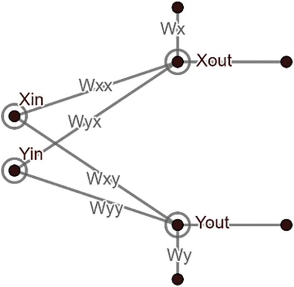
Figure 1: Neural network corresponding to an IFS function

3  Activation Function

Apart from determining the output of the neuron with reference to the values of the weight and input, smoothing out the data to ensure it fits the objective of designing the network is also the purpose of defining the activation function.

Based on their domain, there are various kinds of activation functions for example:

1.    Logistic function ϕ(v)=11+e−av with the domain of [0,1] .

2.    Hyperbolic tangent ϕ(v)=1−e−av1+e−av and algebraic sigmoid function v1+v2 where the domain is [−1,1] .

The logistic growth rate is represented by a in the equations above. As they are beneficial for fractals coding, the sigmoid activation functions will be the focus of this paper.

Based on the IFS coefficients, the fractal image can be segregated into three types.

3.1 Fractals with Positive IFS Coefficients

Represented in the form of a scalar function, this type of IFS results in a neural network output that comprises six weights corresponding to all transformations (IFS) and two units that are calculated from the two input units. Random selection is considered for the iterated function. For each transform, one neuron for the y-coordinate and another for x-coordinate, as well as one coordinate for each fractal image point, are received by all input neurons units. Comprising a biased Sigmoid function [10,12] (Fig. 2), the outputs x and y are returned by each output neuron.

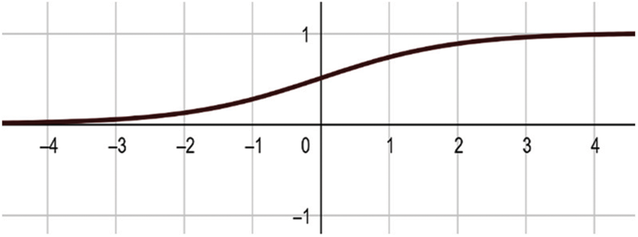
Figure 2: Sigmoid function

The following are the x and y output equations:

Xout=11+e−aWXin (5)

and

Yout=11+e−aWYin, (6)

where the growth rate is a, while

WXin=XinWxx+YinWyxWx, (7)

and

WYin=XinWxy+YinWyy+Wy, (8)

are the weight functions corresponding to the i-th input neuron and j-th output neuron. Meanwhile, the i-th input neuron’s bias is represented by Wi . With random iterations and a large number of points, an image will be attained at the completion of the iterated operation. At this stage, the obtained image is still dissimilar to the desired system image (IFS). Hence, to attain a better target image approximation, updating the neural network’s weights is necessary.

How much the two images differ will affect the weights’ changes. When the weight values are updated, there should be a decrease in the error function, which is measured based on the aforementioned difference.

The Hausdorff distance is the error function that is utilized for the comparison of the two fractal attractors [1,14].

3.2 Fractals with Positive and Negative IFS Coefficients

For this type of IFS, similar procedure and neural network will be utilized. A biased Tan-Sigmoid function is part of the x and y output neuron [10,12] (Fig. 4).

The following are the x and y output equations:

Xout=1−e−aWXin1+e−aWXinandYout=1−e−aWYin1+e−aWYin

Note that similar symbols to the first type of IFS are utilized, with bijk being the IFS coefficients, whereby k = 1, 2, 3, j = 1, 2, and i = 1, 2, …, n. The number of IFS is denoted by n.

Considering different growth rates, Figs. 3, 5 and 7 depict several of the neural networks’ final fractal images with the Tan-Sigmoid function. For this type of fractal, the utilization of a similar error function to the first type of fractal is considered.

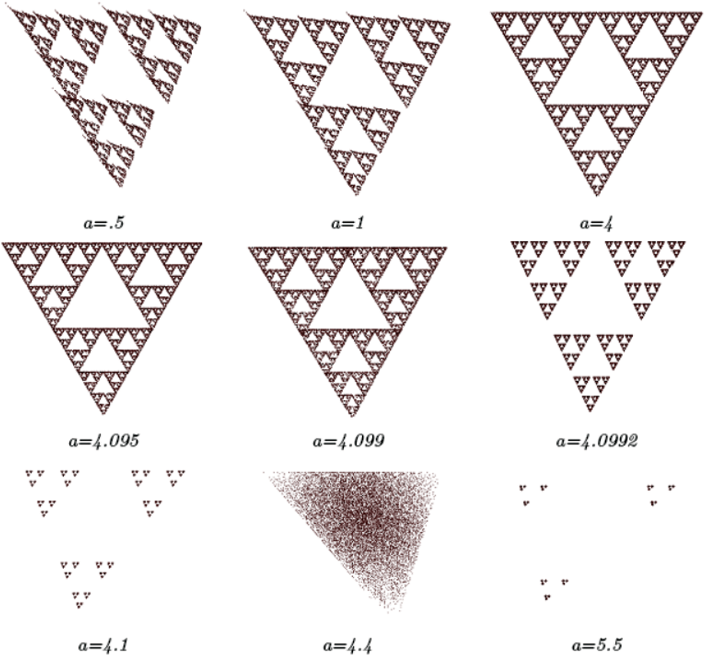
Figure 3: Several final images of a fractal corresponding to the first IFS type for a neural network with varying growth rates

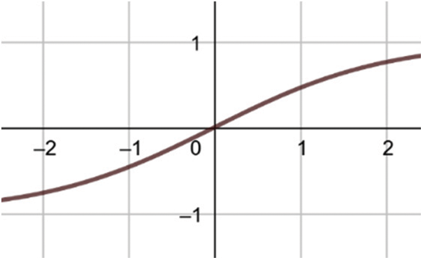
Figure 4: TanSigmoid function

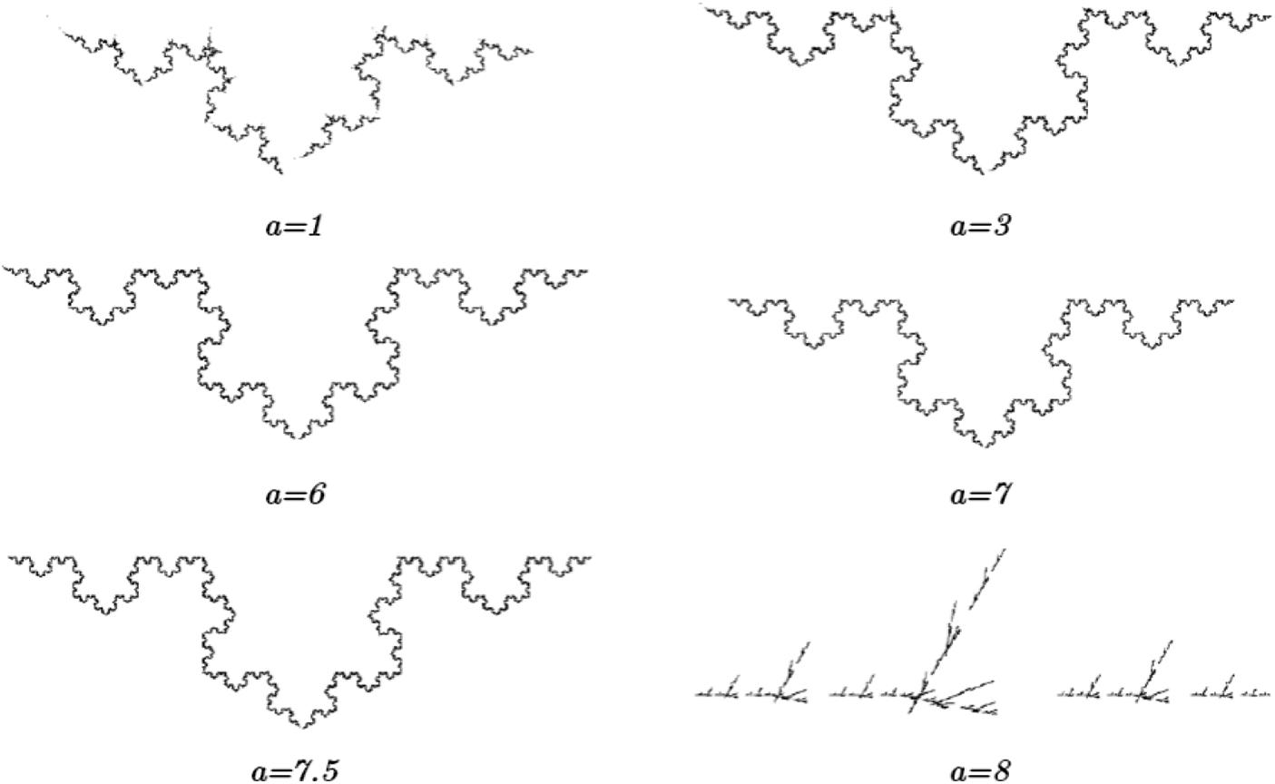
Figure 5: Several fractal output images corresponding to the second IFS type with varying growth rates

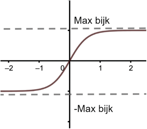
Figure 6: A small change in the Tan-Sigmoid function

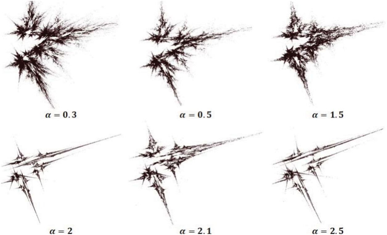
Figure 7: Several output images of fractals for the third type of IFS with varying growth rates

3.3 Fractals with IFS Coefficients bij > 1

If bij is positive, this type of fractal will have a similar activation function to the first IFS type. On the other hand, if bij have both negative and positive values, the activation function will be similar to the second IFS type, where there is only a slight difference between the two cases (Figs. 4 and 6). The following are the x and y output equations:

Xout=max{bijk}1+e−aWXinandYout=max{bijk}1+e−aWYin

or

Xout=max{bijk}1−e−aWXin1+e−aWXinandYout=max{bijk}1−e−aWYin1+e−aWYin.

Both types of IFS consider the use of similar symbols.

4  Future Work

The different types of fractals’ activation functions are the focus of this paper. All types of activation functions and varying growth rates were considered, and their results were studied. For each fractal type, the neural network’s convergence speed to the desired fractal image can be increased for certain growth rate values. With regard to fractal image coding, the activation functions’ relationship with growth rate remains to be an open problem.

Acknowledgement: The author would like to express his gratitude to the ministry of education and the deanship of scientific research–Najran University–Kingdom of Saudi Arabia for their financial and Technical support under Code Number (NU/-/SERC/10/520).

Funding Statement: This research was funded by [Najran University] Grant Number [NU/-/SERC/10/520].

Conflicts of Interest: The author declares that he has no conflicts of interest to report regarding the present study.

References

1. M. F. Barnsley, Fractals Everywhere, San Diego, USA: Academic Press Inc., 1988. [Google Scholar]
2. M. F. Barnsley, V. Ervin, D. Hardin and J. J. Lancaster, “Solution of an inverse problem for fractals and other sets,” Proceedings of the National Academy of Science, vol. 83, no. 7, pp. 117–134, 1986. [Google Scholar]
3. F. Bruno, “Solving the inverse problem for function/image approximation systems II. Algorithm and computations,” Fractals, vol. 2, no. 3, pp. 335–346, 1994. [Google Scholar]
4. T. Q. Tang, Z. Shah, R. Jan, W. Deebani and M. Shutaywi, “A robust study to conceptualize the interactions of CD4+ T-cells and human immunodeficiency virus via fractional-calculus,” Physica Scripta, vol. 96, no. 12, pp. 125231, 2021. [Google Scholar]
5. R. A. Al-Jawfi, “The effect of learning rate on fractal image coding using artificial neural networks,” Fractal Fract, vol. 6, no. 280, pp. 1–9, 2022. [Google Scholar]
6. J. Hart, “Fractal image compression and the inverse problem of recurrent iterated function systems,” IEEE, Computer Graphics and Applications, vol. 16, no. 4, pp. 25–32, 1996. [Google Scholar]
7. L. Fausett, Fundamentals of Neural Networks: Architectures, Algorithms and Applications, India: Pearson Education, 2006. [Google Scholar]
8. C. L. Giles, C. B. Miller, D. Chen, H. H. Chen, G. Z. Sun et al., “Learning and extracting finite state automata with second-order recurrent neural networks,” Neural Computation, vol. 4, no. 3, pp. 393–405, 1992. [Google Scholar]
9. S. P. Siregar and A. Wanto, “Analysis of artificial neural network accuracy using backpropagation algorithm,” International Journal of Information System & Technology, vol. 1, no. 1, pp. 34–42, 2017. [Google Scholar]
10. G. E. Hinton, D. E. Rumelhart and R. J. Williams, “Learning internal representations by error propagation, parallel distributed processing,” Explorations in the Microstructure of Cognition, vol. 1, no. 1, pp. 318–362, 1986. [Google Scholar]
11. O. S. Melnik, “Representation of information in neural networks,” Ph.D. Thesis, Brandies University, Waltham, USA, 2000. [Google Scholar]
12. J. B. Pollack, “The induction of dynamical recognizers,” Machine Learning, vol. 7, pp. 123–148, 1991. [Google Scholar]
13. D. P. Bertsekas and J. N. Tsitsiklis, Neuro-Dynamic Programming, Belmont, Mass: Athena Scientific, 1996. [Google Scholar]
14. Y. LeCun, P. Y. Simard and B. Pearlmetter, “Automatic learning rate maximization by on-line estimation of the hessian’s eigenvectors,” In: S. J. Hanson, J. D. Cowan and C. L. Giles (Eds.) Advances in Neural Information Processing Systems, 5, San Mateo, CA: Morgan Kaufmann, vol. 5, pp. 156–163, 1993. [Google Scholar]
15. T. K. Leen and G. B. Orr, “Using curvature information for fast stochastic search,” Advances in Neural Information Processing Systems, vol. 9, pp. 606–612, 1997. [Google Scholar]
16. C. Darken and J. Moody, “Towards faster stochastic gradient search,” Advances in Neural Information Processing Systems, vol. 4, pp. 1009–1016, 1992. [Google Scholar]
17. W. J. Braverman and L. Yang, “Obtaining adjustable regularization for free via iterate averaging,” in Int. Conf. on Machine Learning, pp. 10344–10354, 2020. https://researchr.org/publication/icml-2020 [Google Scholar]
18. H. J. Kushner and G. Yin, Stochastic Approximation Algorithms and Applications, New York: Springer-Verlag, 1997. [Google Scholar]
19. J. E. Hutchinson, “Fractals and self-similarity,” Indiana University Mathematics Journal, vol. 30, no. 4, pp. 713–747, 1981. [Google Scholar]
20. R. A. Al-Jawfi, “Nonlinear iterated function system coding using neural networks,” Neural Network World, vol. 16, no. 4, pp. 349–352, 2006. [Google Scholar]
21. A. H. Ali, L. E. George, A. A. Zaidan and M. R. Mokhtar, “High capacity, transparent and secure audio steganography model based on fractal coding and chaotic map in temporal domain,” Multimedia Tools and Applications, vol. 77, no. 23, pp. 31487–31516, 2018. [Google Scholar]
Cite This Article
Copyright © 2023 The Author(s). Published by Tech Science Press.
This work is licensed under a Creative Commons Attribution 4.0 International License , which permits unrestricted use, distribution, and reproduction in any medium, provided the original work is properly cited.
Downloads
Citation Tools