Machine Learning-Based Threatened Species Translocation Under Climate Vulnerability

1  Introduction

Climate change has a significant impact on the distribution of taxa and the phenology of their flowers and fruits across the world. Species are impacted both directly and indirectly by global change factors, which influence both individuals and populations. Habitat loss, agricultural expansion, urbanization, a rise in illness, pollution, overexploitation, and predation are some of the factors that have an impact on species [1,2]. In response to the distorted temperature and precipitation regime, some plant species and other categories of taxa are shifting their geological range. As of 2020, the Intergovernmental Panel on Climate Change (IPCC) anticipated that global warming would be 1.5 degrees Celsius and relative precipitation would increase, resulting in the extinction of 20–30 percent of all world species [3], based on current knowledge.

It has been extensively established that the earth’s atmosphere has warmed by 6 degrees Celsius during the previous 100 years [4]. It is possible that the fast increase in temperature over the course of the century will have a significant impact on ectotherm creatures such as reptiles. Environmental factors and ecological circumstances have an impact on the geographical distribution, reproductive success, physiological performance, and behavior of animals [5]. The activities are accomplished by the use of the species’ body temperature in proportion to the surrounding environment’s temperature. Researchers have shown that when nests are exposed to increasing temperatures, it results in substantial alterations in the sex ratio when compared to species that are found in protected areas [6], according to their findings. The amount of clutch produced is dependent on variations in temperature, which might be either rising or decreasing [7]. According to [8], the influence of climatic change on reptiles’ life cycle and body size is taken into consideration.

Climate change does not have a direct impact on the organisms themselves. However, the combined influence of environmental variables has significant consequences for species. Both biotic and abiotic factors have an impact on the organism directly. The most evident characteristics of climate change include phenology, fecundity, and survival [9], which are among the many components of climate change. Climate conditions are always fluctuating, resulting in the reshuffling and gathering of species within environmental groups, which is characterized by unpredictable behavior.

This results in the establishment of a species’ habitat, the expansion of the habitat’s size, or the extinction of the species in that location. Threatened and endangered species are typically environment specialists and comparably extraordinary individuals; as a result, they are likely to be disproportionately harmed by climate change [10]. The preservation of species within their current ranges may prove to be a difficult task. The identification and protection of critical habitats is an important strategy in the conservation of endangered species. Developing an adaptation plan for the protection of ecosystems and species is becoming more vital as global climate change continues.

In order to evaluate the susceptibility of an ecosystem and species, several vulnerability assessment techniques have been created. Bioclimatic modeling [11] will be the most effective modeling tool for assessing biodiversity in that tool. According to the findings of this research, climate change will have a negative impact on vulnerable and endangered species, as well as ecological and genetic diversity. In addition, we built a decision support system for managing biodiversity by using a climate modeling approach to predict the distribution of endangered and vulnerable species [12] under climate change. In conclusion, conservation measures based on climate change and species risk status, and the preservation of ecosystem services are recommended.

2  Materials

The International Union for Conservation of Nature (IUCN) collects data on reptile species in order to identify those that are vulnerable or endangered. The International Union for Conservation of Nature (IUCN) provided a comprehensive list of reptile species and features. The life history, as well as extrinsic and intrinsic characteristics, as well as environmental information, is gathered from the Encyclopedia of Life (EOL). For further research, species having IUCN [13] statuses of vulnerable or endangered species were selected from the reptile dataset for consideration. To depict current environmental conditions and investigate the relationship between bioclimatic conditions and species distribution patterns, a bioclimatic data set of raster-based bioclimatic variables were derived from the WorldClim datasets and used to represent the current environmental conditions and discover the relationship between species distribution patterns.

The WorldClim Delta Method technique delivers climate forecasts [14] that have been statistically downscaled to a geographic resolution that is nearly equal to the equator. The temperature and precipitation readings were used to create the bitmaps of climatic variables, which were then divided into a monthly periodical, seasonal, and yearly trends. The variables listed above were used to describe the current environmental conditions and analyze the relationship between bioclimatic conditions and species distribution patterns in order to complete this study [15]. WorldClim’s future climate projections include eight new sets of assumptions, as well as two new sets of assumptions [16], such as greenhouse gas concentrations for future concentrations and atmospheric components downscaled using the single adoption technique, for the future climate projections [17].

3  Methods of Classifier

The LFMSs (VLF(t)) can be depicted as in Eq. (1)

vLFM(t)={aexp⁡(jπγt2);0≤t≤To0;T0<t<TPRI (1)

where, a-amplitude, γ-sweep rate’s frequency, To -duration of pulses and TPRI-PRIs. Frequency of LFMSs varies with time where immediate frequency is computed using fi(t)2=γt . mth pulse when MLFM pulses burst can be represented as time shift forms of LFMSs and shown in Eq. (2)

vj(t)=v(t−nTPRI)for0≤t≤To (2)

where, n∈[0,1,...,N−1] and N represents total pulses count in a burst. vj(t) gets modulated by high frequency carrier signals where modulations can be represented mathematically as Eq. (3)

v(t)={vj(t)}exp⁡(j2πfct) (3)

where, fc -carrier signal’s frequency. Returning signals pm(t) are time delayed variants of v(t) where τm stands for TDEs of the mth pulse when Eq. (4) is satisfied,

τm=τo−2C{vmTPRI} (4)

where τo -first pulse’s TDE, v-radial velocity, and c–light’s velocity. For maintaining generality of target time (N pulses) v is considered constant or constant [18] Doppler shifts are assumed. Then Time differences 2/c { vm TPRI} in time shifts of return signals when targets change positions over nTPRI results in subsequent changes to pn(t) and given by Eq. (5),

pn(t)={vj(t−τn)}exp⁡(j2πfc(t−τn))+km(t) (5)

where, km(t) -additive thermal noises Returning signals, pn(t) , of basebands when depicted mathematically, form Eq. (6),

pm(t)={vj(t−τn)}exp⁡(−j2πfcτn)+km(t) (6)

Which implies Pn(f) can be written as Eq. (7),

Pn(f)=|VLFM(f)|2exp⁡(−j2πfcτn)exp⁡(−j2πfτn)+km(f) (7)

where, VLFM(f) represents Fourier transforms LFMSs Sampling frequency l=[0,1,..,L−1] with interval Δf and dividing by |VLFM(lΔf)|2 yields the following Eq. (8)

p(n,l)=exp⁡(−j2πfcτn)exp⁡(−j2πΔfτn)+k(n,l) (8)

where k(n, l) represents thermal noise’s discrete samples. Substituting τn from Eq. (4) results in Eq. (9),

p(n,l)=exp⁡(j2πnfdTPRI)exp⁡(−j2πlΔfτo)exp⁡(j2πfdml(TPRIΔffc))+k(n,l) (9)

where fc= 2vfc/c represents unknown Doppler shifts caused by target radial velocities. From Eq. (9), it can be noted that returning signals, r(m, l), are nonlinearly and exponentially related to TDEs ( τo and fd ) which are estimated from returning signals r(m, l) using EKFs and UKFs. Gaussian filters were used instead of particle filters as result in acceptable estimation with low processing costs. The suggested EKFs and OIUKFs for estimating TDEs are Gaussian filters. The LFM radar system states assessment model was developed using Bayesian framework followed by EKFs and OIUKF estimations for τo and fd .

This study uses notations for mathematical representations where constants are in upper cases, Vectors are boldfaced upper cases, superscript representations are: ( T transposes. H complex conjugate transposes of matrices and * scalar complex conjugate operations), statistical expected outcomes are represented by E[⋅] . R denotes real numbers while C stands for complex numbers where ℜ (·) implies real parts and ℑ (·) stands for imaginary parts.

This work proposed state assessments include measurements models where the states are measured using mathematical links. TDEs ( τo and fd ) form the state, while the observed values (returning signals p(n, l)) constitute measurements and variables declared included x=[τofd]T and y=[ℜ(r(m,l))ℑ(r(m,l))]T . The state space model defined rise consistently in intervals and TDEs due to assumed constancy of radial velocities. Errors arising from this study assumptions of constants are treated as process noises. The modelled state can be depicted mathematically as Eq. (10),

yk+1=f(yk)+ηk=yk+Δy+ηk (10)

where k∈{1,2,…,K} , K=ML stands for discretized sample counts of signals returned, and Δx=[ToK,0] represents changes/shifts between successive returning signals. ηk represents noises that are additive and assist in modelling error compensations. Based on Eq. (10), measurements ( xk+1 ) can be depicted as Eq. (11),

xk+1=c(xk+1)+dk+1=[R(exp⁡(j2πnyk+1(2)TPRI)exp⁡(−j2πlΔfyk+1(1))exp⁡(j2πyk+1(2)ml(TPRIΔffc)))I(exp⁡(j2πnyk+1(2)TPRI)exp⁡(−j2πlΔfyk+1(1))exp⁡(j2πyk+1(2)ml(TPRIΔffc)))]+vk+1 (11)

where, dk stands for noises measured. These measurements help mitigate signal errors that occur while collecting/processing them. ηk , vk represent Gaussian filter’s assumed zero means with covariance Qk and Rk. This study considers additive impacts of process/measurement noises.

Bayesian filtering are two step operations using predictions and updates:

This phase creates the PDFs (Probability Distribution Functions) of states one time step forward (relation to the available observations) by utilising Chapman–Kolmogorov given as Eq. (12),

P(yk|x1:k−1)=∫P(yk|yk−1)P(yk|x1:k−1)dyk−1 (12)

where P(·) stands for PDFs and P(yk|x1:k−1) stands for prior PDFs.

PDFs are reconstructed in this step when new measurement values from Bayes rule [19] yk are received and depicted as Eq. (13),

P(xk|y1:k−1)=P(xk|y1:k−1,yk)=1/ckP(yk|xk)P(xk|y1:k−1) (13)

ck=P(yk|y1:k−1)=∫P(yk|xk)P(xk|y1:k−1)dxk (14)

where, P(yk|xk) stands likely measures achieved using Eq. (14) and ck represents constant for normalizations. The use of Bayesian filtering results in the construction of posterior PDFs P(xk|y1:k).

The estimations of TDEs ( τo and fd ) from returning signals, r(m, l) of the investigated RSs using are simplified from states assessment as estimations of x k from known y k measurements where EKFs are analytical simplifications of Bayesian frameworks and where conditional PDFs in Bayesian frameworks [15] are assumed to be Gaussians as shown in Eq. (15),

P(xk|k−1)∼N(xk|k−1;x^k|k−1,Pk|k−1) (15)

P(xk|k)∼N(xk|k;x^k|k,Pk|k) (16)

where, real Gaussian distributions are represented as N, xk|k−1 stands for mean values while Pk|k−1 implies covariance of xk|k−1 and similarly xk|k implies mean values and Pk|k covariance of xk|k . xk|k−1 and Pk|k−1 are predicted while xk|k and Pk|k are updated as detailed below in Eq. (16):

In this step, prior PDFs ( xk|k−1 and Pk|k−1 ) result when Jacobian (Fk) of f(xk) ((11)–(12)) is used and depicted as Eq. (17),

Fk=∂f(x)∂x|x=x^k−1|k−1=[1001] (17)

In the initial part of this step, measurements (y^k|k−1) are predicted along with error covariance ( Pk|k−1YY ) using Jacobian (Hk) of h(·) which results in new measurements yk . Subsequently posterior estimates and covariances, x^k|k−1 and Pk|k , are obtained using Kalman filter gains ( Kk ) where posterior estimations x^k|k=[τ^okf^dk]T results desired TDEs and Doppler shift outcomes in Eq. (17).

The calculation of an IUKF using the Fisher estimation framework is described in [15], and it entails minimising the following cost function in the filter’s measurement update phase in Eq. (18),

y^t|t=argminy⁡Z(y)=argminy12fT(y)f(y) (18)

f(y)=[Rt−12(yt−h(x))Pt|t−1−12(x^t|t−1−x)] (19)

Hi=(Pixy)TP−1 (20)

It presupposes, like the IUKF version, that the measurement function is affine in the vicinity of x and x i, and therefore that hx′(x) = hx′(xi) = Hi. The Jacobian Hi is not explicitly computed in the UKFs, but the fact that Pxy = PHT in the linear case may be used to infer a stochastic linearization. As a result, equation provides a fair estimate of Hi in the IUKF in Eqs. (19) and (20),

When P symmetry has been exploited and Pxy implicitly incorporate second order transformation effects. The state iteration in IUKF may be utilised to generate the following equation using the preceding stochastic linearization approach Eq. (21),

xi+1=x^+Ki(y−y^i−(Pixy)TP−1(x^−xi)) (21)

Ki=Pixy(Piyy)−1 (22)

y^i=∑k⁡W(k)Yi(k) (23)

It can be utilised as a starting point in the IUKF It’s worth noting that y = y(t|t − 1) remains constant. The projected measurement y i must still be determined. Equation can be used to express two different natural alternatives Eq. (23),

y^i∗=Yi(0) (24)

i.e., the converted centre sigma point, represented by the superscript * in this case. Two somewhat different interpretations of the cost function by equation result from the two options Eqs. (25) and (26).

V(x)=(yt−E[h(x)])TRt−1(yt−E[h(x)])+(x^t|t−1−x)TP(t|t−1)−1(x^t|t−1−x) (25)

V∗(x)=(yt−h(x))TRt−1(yt−h(x))+(x^t|t−1−x)TP(t|t−1)−1(x^t|t−1−x) (26)

both depict different approximations of costs where corrections to states can result in decreased costs i.e., V(xi+1)<V(xi) . If this is not the case a step size parameter α by Eq. (27).

yj+1=yj+αj(y^−yj+Gj(x−x^j−Hi(x^−xi))) (27)

MCEHOs are used to compute the step sizes where EHOs (Elephant Herding Optimizations) uses both global and local searches. Local searches, on the other hand, aim to locate better step sizes in smaller search spaces with smaller promising approximate predictions of time and Doppler flaws. Elephant’s herding behaviours are characterised as elephant populations (with varying step sizes) split into clans. Generations have males which leave their clans for optimal selections of step sizes. Clans represent local searches in the algorithm through the optimum selection of step sizes, but male elephants leaving clans are global search implementations through step sizes. Matriarchs are solution (elephants) in the clan with the best fitness values for TDEs. Moving male elephants, on the other hand, are solutions τo and fd with the worst fitness function of RSs. MCEHOs approach divides Elephant population into k clans which are D-dimensional solutions created randomly in search spaces by using lower bounds xmin and upper bounds xmax of TDEs and using Eq. (28),

x=xmin+(xmax−xmin+1)rand (28)

where, rand implies random numbers between (0,1). New solutions get generated in generations when clan members (j) from clan (ci) with best fitness values get attracted by solutions ( xbest,ci ) in Eq. (29):

xnew,ci,cj=xci,cj+αmutation(xbest,ci−xci,j)rand (29)

where, xnew,ci,cj -j new solution in clan ci for optimal selection of steps size in TDEs and droppler effects, xci,cj -previous generation’s solution, αmutation -generated parameter via mutation operator and algorithm’s parameter is set correspondingly for TDEs and droppler effect. If the mutated value is worse than the new value that is created via new mutated value. rand∈[0,1] random numbers between (0,1) in uniform distributions. Scaling factor α influences best TDEs and doppler effect values with their step sizes and these positions in clans get updated based on Eq. (30) given below:

xnew,ci=βxcenter,ci (30)

where [0,1] is the second algorithm parameter, which determines the clan centre effect. xcenter,ci for TDEs and droppler effect. Clan center is defined by Eq. (31),

xcenter,ci,d=1nci∑l=1nci⁡xci,l,d (31)

where 1 ≤ d ≤ D represents the dth dimension and nci is the number of reduced TDEs and droppler effect in clan ci . In each clan, nci solutions with the worst fitness values for TDEs and droppler effect of the clan ci are chosen to be replaced by the following Eq. (32),

xworst,ci=xmin+α(xmax−xmin+1)rand (32)

where xmin and xmax represent lower and upper bounds of search spaces for TDEs and doppler effects in the interval rand ∈ [0,1] TDEs and the doppler effect were used to represent a random integer from uniform distributions where they use two separate one-dimensional maps, circles and sinusoidal maps, to generate random numbers. The circular maps can be described by Eq. (33),

yg+1=[yg+a−b2πsin⁡(2πyg)]mod1 (33)

where the produced chaotic sequence is inside b = 0.5 and a = 0.2 (0, 1). The equation for a sinusoidal map is Eq. (34),

yg+1=byg2sin(πyg) (34)

where for b = 2.3 and y0 = 0.7 the following simplified form.

4  Result and Discussion

For all species, GLM-based species distribution models were created to forecast whether a species will be present in any given grid cell and the chance of that species being there. With a binomial answer, the probability, which runs from 0 to 1, necessitates the use of a cut-off number to identify whether a cell is present or absent. The sensitivity (number of properly predicted presences) and specificity (number of correctly predicted absences) are used to determine the cutoff value between 0 and 1 (number of correctly predicted absences).

The Fig. 1 shows the species presence data, based on bioclimatic variables. The variables show the occurrence record of species. The rho implies the strength of correlation and p value for the variable along with the sample size. Most of the species translocated from source place to outside the historical range. A huge amount of taxon moved towards to the outside the range because of the local extinctions at historical range. For these species, we calculated the decrease in the source range to new place as the amount of dispersal, and this value divided by the time between local extinction rather than movement of individuals. The recent survey and studies predict that the global climate change driven by human activities, which is likely to be increase in the future.

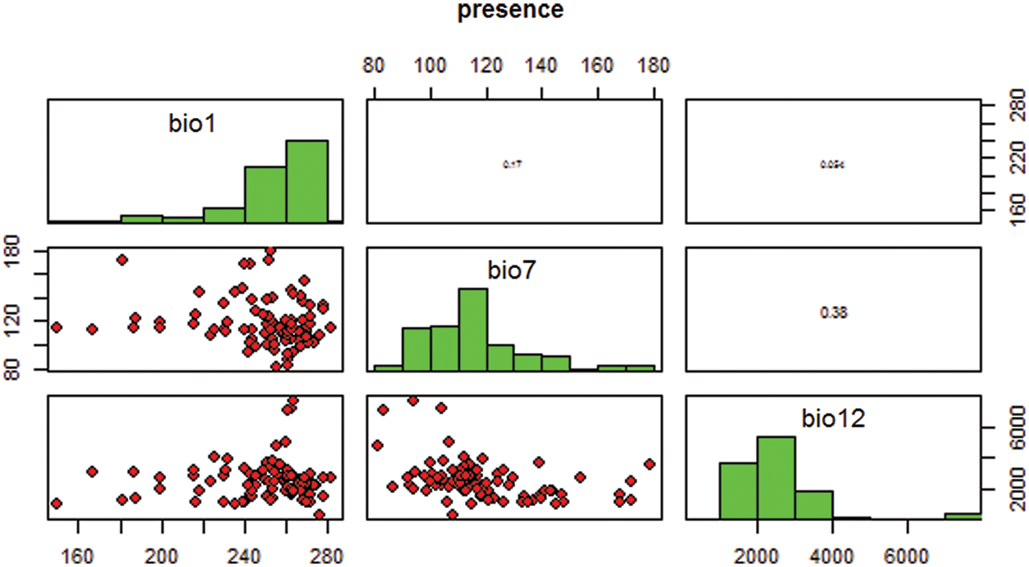
Figure 1: Presence of species using bioclim variables

Figs. 2 and 3 depict the distribution of species depending on species characteristic and climatic factors, respectively. This global climate change is occurring as a result of the fact that the majority of species have moved their geographic location and relocated their existing distribution. We may infer some general conditions for the introduction of species to a new place from the decision support system that we discussed before. Using a given species I strategy (j), and location (k), our decision support system can determine if reintroduction is necessary to protect the species or whether the species can survive in its existing range.

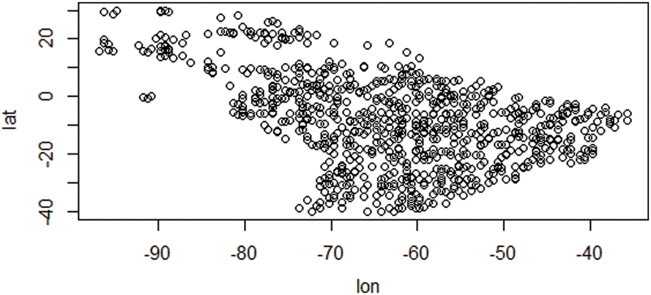
Figure 2: Species occurrence data

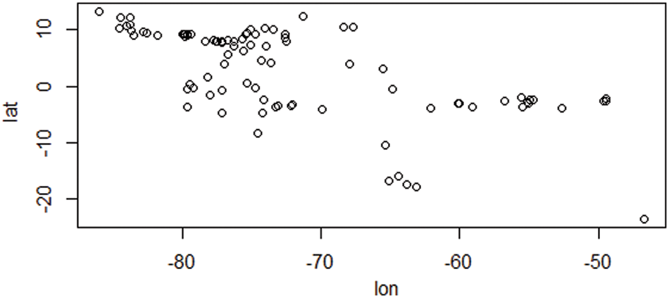
Figure 3: Species distribution based on future climate change

Instead of historical range size, the mature body size and body mass of a species are also statistically significant predictors of extinction risk. Based on the likelihood of extinction and restricted confidence intervals, the evidence presented in the findings suggests that the species is likely to go extinct in the wild in the near future. Only a subset of species that are susceptible to climate change will benefit from the reintroduction of animals from their historical range to a preferred site based on future climatic projections. It has been done in the past with closely related taxonomic species in order to determine the efficient component of extinction forms and the population isolation from reintroduced predators for conservation purposes.

Fig. 4 depicts the model evaluation that was carried out to demonstrate the correctness and usefulness of the study. According on the study’s purpose and the quality of a forecast for abundance data, numerous metrics are used to assess the results. A large variety of metrics for assessing models based on presence-absence or presence-only data are threshold dependent, making them particularly useful. Predicted values that are higher than that threshold indicates a forecast of presence, whereas predicted values that are lower than that threshold suggest absence. Some metrics place more emphasis on the importance of fake absences, while others place greater emphasis on the importance of false presences.

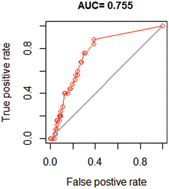
Figure 4: Predicted model evaluation using area under the receiver operator curve (AUC)

The correlation coefficient and the area under the curve (AUC) are two often used statistics that are not reliant on a threshold. When dealing with unbalanced data, a large AUC suggests that sites with high projected suitability values are more likely to be places where the species is known to be present, while sites with lower model prediction values are more likely to be areas where the species is unknown to be present. An AUC score of 0.5 indicates that the model is as excellent as a random guess in terms of performance. In this section, we demonstrate how to compute the correlation coefficient and the AUC using two random variables.

Presence has higher values and represents the predicted value for known locations where the species is present, while absence has lower values and represents the predicted value for known locations where the species is absent. Presence has higher values and represents the predicted value for known locations where the species is present. Our model architecture is easily adaptable to future choices to reintroduce the species for conservation purposes, and it can do so without difficulty. The model is being suggested to complement the revised International Union for Conservation of Nature recommendations for reintroductions and other conservation of species that have been translocated outside of their original range. Additional events and outcomes associated with the key species under consideration for conservation reintroductions are taken into account by the decision-support framework for conservation reintroductions.

5  Conclusion

Protection science has made considerable strides in the development of an applied field that aids in the making of better choices for the conservation of ecosystems, which is now under development. Climate change, on the other hand, as well as widespread disturbance, make conservation efforts more difficult. As a result, models of habitat appropriateness that may be used to assess the vulnerability of vulnerable and endangered species are required. Based on several linear regressions, our model demonstrated that the range contraction of climatically adequate natural habitats for vulnerable and endangered species is very expected in the near future. Managing climate change has the potential to be an important adjustment approach for the conservation of ecosystems in the future. In conclusion, we propose that appropriate habitat management of current protected areas, as well as an increase in the number of protected areas, might help to lower the danger of extinction in the future.

In addition, endangered animals should be relocated to safe havens where they may continue to thrive in the long term. Many reptile species are threatened by climate change, which is becoming more severe. There would be a need for cautious, well-considered planning that takes a long-term perspective in order to cope with these difficulties. The participation of interested parties from the government and nonprofit organizations, as well as representatives from a number of sectors, is required in order to achieve this goal. Further study should concentrate on the spatial forecast of these reptiles both inside and outside protected areas, taking into account the unknown or unrecorded species, poaching activities, interactions with humans and wild life, and model updating for conservation planning, among other factors.

Acknowledgement: Thank you for the guide and Reviewers.

Funding Statement: The authors received no specific funding for this study.

Conflicts of Interest: The authors declare that they have no conflicts of interest to report regarding the present study.

References

1. C. Macinnis, A. R. Mcintosh, J. M. Monks, N. Waipara and S. White, “Climate-change impacts exacerbate conservation threats in island systems: New Zealand as a case study,” Frontiers in Ecology and the Environment, vol. 19, no. 4, pp. 216–224, 2021. [Google Scholar]
2. G. Sahar, K. A. Bakar, S. Rahim, N.A.K.K. Khani and T. Bibi, “Recent advancement of data-driven models in wireless sensor networks: A survey,” Technologies, vol. 9, no. 4, pp. 76, 2021. [Google Scholar]
3. M. K. Watfa, S. Selman and H. Denkilkian, “Uw-Mac: An underwater sensor network mac protocol,” International Journal Communication System, vol. 23, no. 4, pp. 485–506, 2010. [Google Scholar]
4. F. A. Alfouzan, A. Shahrabi, S. M. Ghoreyshi and T. Boutaleb, “A collision-free graph coloring MAC protocol for underwater sensor networks,” IEEE Access, vol. 7, pp. 39862–39878, 2019. [Google Scholar]
5. H. Mei, H. Wang, X. Shen and W. Bai, “An adaptive MAC protocol for underwater acoustic sensor networks with dynamic traffic,” in OCEANS 2018 MTS/IEEE, Charleston, pp. 1–4, 2018. [Google Scholar]
6. Y. F. Qu and J. J. Wiens, “Higher temperatures lower rates of physiological and niche evolution,” Proceedings of the Royal Society B: Biological Sciences, vol. 287, no. 1931, pp. 20200823, 2020. [Google Scholar]
7. X. Zhuo, F. Qu, H. Yang and Y. Wu, “Time-based adaptive collision-avoidance real-time MAC protocol for underwater acoustic sensor networks,” in Proc. of the Thirteenth ACM Int. Conf. on Underwater Networks & Systems, Shenzhen China, pp. 1–5, 2018. [Google Scholar]
8. A. R. Cho, C. Yun, Y. K. Lim and Y. Choi, “Asymmetric propagation delay-aware TDMA MAC protocol for mobile underwater acoustic sensor networks,” Applied Sciences, vol. 8, no. 6, pp. 962, 2018. [Google Scholar]
9. E. Khatter and D. Ibrahim, “Proposed ST-Slotted-CS-ALOHA protocol for time saving and collision avoidance,” The ISC International Journal of Information Security, vol. 11, no. 3, pp. 67–72, 2018. [Google Scholar]
10. X. Liu, X. Du, M. Li, L. Wang and C. Li, “A MAC protocol of concurrent scheduling based on spatial-temporal uncertainty for underwater sensor networks,” Journal of Sensors, vol. 21, no. 1, pp. 112, 2021. [Google Scholar]
11. G. H. Mathes, J. van Dijk, W. Kiessling and M. J. Steinbauer, “Extinction risk controlled by interaction of long-term and short-term climate change,” Nature Ecology & Evolution, vol. 5, no. 3, pp. 304–310, 2021. [Google Scholar]
12. X. de Lamo, M. Jung, P. Visconti, G. Schmidt-Traub, L. Miles et al., Strengthening Synergies: How Action to Achieve Post-2020 Global Biodiversity Conservation Targets can Contribute to Mitigating Climate Change. Cambridge, UK: UNEP-WCMC, 2020. [Google Scholar]
13. B. R. Scheffers and G. Pecl, “Persecuting, protecting or ignoring biodiversity under climate change,” Nature Climate Change, vol. 9, no. 8, pp. 581–586, 2019. [Google Scholar]
14. O. Hoegh-Guldberg, D. Jacob, M. Taylor, T. G. Bolaños, M. Bindi et al., “The human imperative of stabilizing global climate change,” C. Science, vol. 365, no. 6459, pp. 1263–1274, 2019. [Google Scholar]
15. S. E. Fick and R. J. Hijmans, “WorldClim 2: New 1-km spatial resolution climate surfaces for global land areas,” International Journal of Climatology, vol. 37, no. 12, pp. 4302–4315, 2017. [Google Scholar]
16. T. M. Rout, E. McDonald-Madden, T. G. Martin, N. J. Mitchell, H. P. Possingham et al., “How to decide whether to move species threatened by climate change,” PloS One, vol. 8, no. 10, pp. e75814, 2013. [Google Scholar]
17. J. C. Deb, S. Phinn, N. Butt and C. A. McAlpine, “Adaptive management and planning for the conservation of four threatened large Asian mammals in a changing climate,” Mitigation and Adaptation Strategies for Global Change, vol. 24, no. 2, pp. 259–280, 2019. [Google Scholar]
18. E. E. Saupe, A. Farnsworth, D. J. Lunt, N. Sagoo, K. V. Pham et al., “Climatic shifts drove major contractions in avian latitudinal distributions throughout the Cenozoic,” The Proceedings of the National Academy of Sciences (PNAS), vol. 116, no. 26, pp. 12895–12900, 2019. [Google Scholar]
19. C. S. Sevillano-Ríos and A. D. Rodewald, “Avian community structure and habitat use of Polylepis forests along an elevation gradient,” PeerJ, vol. 5, no. 2, pp. 3220, 2016. [Google Scholar]
Cite This Article
Copyright © 2023 The Author(s). Published by Tech Science Press.
This work is licensed under a Creative Commons Attribution 4.0 International License , which permits unrestricted use, distribution, and reproduction in any medium, provided the original work is properly cited.
Downloads
Citation Tools