Popularity Prediction of Social Media Post Using Tensor Factorization

1  Introduction

In the present scenario, social media platforms are very popular. Thousands of millions of messages and contents are generated every day on platforms like Facebook, Behance, Instagram, etc. Due to the substantial traffic available on these platforms, popular content extraction is the major challenge in the present life. The popular content is useful for both the owner and follower in these platforms. The popularity of social media content is very useful for increasing visibility, turnover, and sales so on. The popularity of social media platforms is estimated by different parameters like several followers, comments, likes, and shares, etc. for the post.

The essential advantages of the popularity prediction of content are to improve the experience of the user, broad area applications, and effectiveness. The sharing time of any content on the social media platform reflects the popularity of that content. The prediction of popularity of social media content is configured by two approaches: feature-based and generative based. The feature-based strategies work with the machine learning process and extract various attributes from the content. The characteristics like temporal and structural content are used to train the model of machine learning classifiers. In generative approaches, a model is developed, which classifies the content based on factorization. The model extracts small information related to the content and predicts the popularity of that. The predicting power is not very efficient in generative methods of popularity prediction. The prediction power is improved using the deep learning methods, which achieve feature information from the content [1]. The generative-based methods detect distribution changes and update the model. The overfitting problem is also minimized in the case of generative-based methods.

The various users or followers monitor the content or post on the social media platform. The information related to the content distributes among the people who follow their pages. The data presented on the social media platform is massive, which can be used for predicting the popularity of various categories of content like video, audio, images, text, etc. The online social media content popularity is categorized into two levels; 1) user-level popularity and 2) population-level popularity. The user-level popularity deals with the nature of users who react to the posted content. In this scheme, some entries or information are missing, which is costly to configure. On the other, the number of users reacting to the posted content will define popularity. Some unidentified information regarding the user’s nature and interest may affect the flexibility condition. In [2], a group-level popularity prediction is provided within the group of users.

In a group-level scheme, the popularity is predicted in a group or cluster where all users have the same interest. The content posted in that group easily reflects the attraction among the group users. So, the future popularity prediction of group posts is estimated accurately and less costly. The time series forecasting method is implemented for the historical data popularity prediction in [3]. A trend prediction method is employed in [4] for the popularity of the casting of tweets related to crime on Twitter. Similarly, online news data popularity prediction was performed by the Intelligent Detection Support System (IDSS) for the Mashable database in [5].

We experimented the user-level, population-level and group-level popularity prediction with the Behance dataset, which is a social media platform for sharing the projects. We have experimented with the popularity prediction of 30-time stamps by user-level [6], population-level [7] and our scheme. Fig. 1 compares these three scheme’s predictions with ground truth.

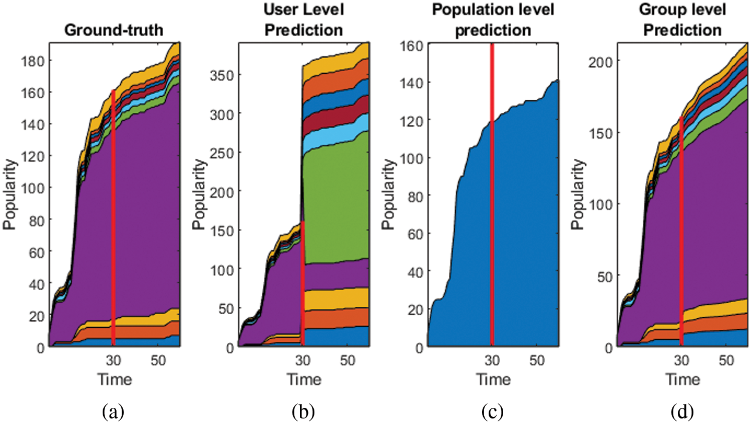
Figure 1: (a) ground truth data (b) prediction by user-level [6], (c) prediction by population level [7] (d) prediction by group-level proposed scheme

We have followed the prior k-level clustering step before tensor-based factorization in all of the above schemes. It is demonstrated by this comparison that the user-level method is noisy when it comes to compensating the user’s behavioral change. The population-level has given a coarser view. The prediction by group-level is the winning method. Keeping these points into consideration, the motivation of the work in this article is:

•   The prediction of the social media post’s popularity is affected by uncontrolled external factors, which affect the prediction accuracy significantly.

•   The user-level and group level prediction methods give a coarser view of the popularity and are backed by the uncertain noises in the data

•   The data from social media is multidimensional and analysis of it considering it in 2-dimension as with multiple attributes lacks the dependency analysis of every attribute.

The PARAFAC is the most stable factorization scheme amongst others like CANDECOMP/PARAFAC, tucker, Support Vector Decomposition (SVD) [8]. In the prediction of data, unexpected changes in the pattern may arise and are stated as noise. The conventional PARAFAC is unable to counter that. Various other factorization methods like graph partition [9], simultaneous tensor decomposition and completion (STDC) [10], Tailored optimization algorithm for low rank tensor recovery [11], Stochastic Gradient Descent method for expected tensor decomposition [12] have worked to improve the PARAFAC. These algorithms have been developed to solve prediction problems or generate the missing data. Few researchers have also followed the clustering of the data as preprocessing step followed by the heuristic optimization too. The prediction of the popularity data is developed on the line of action of the missing data imputation also. This article proposes an improved advance-PARAFAC (A-PARAFAC) that can deal with this noise. The Adam optimizer is used to optimize the factors for minimum error along with bias addition in the factors to avoid the local minima point. The bias stability is enhanced through logistic mapping.

For this, the modified adam optimization is proposed in this article. The primary contribution in this social media popularity prediction work is:

•   Group-level popularity prediction by hierarchically clustering the similar data by recursive graph way clustering scheme.

•   Capturing the future changes in user’s wisdom to rate the project/product by introducing the bias in the PARAFAC decomposition.

•   Modifying the Adam optimization to continuously update the bias factors to get the converging solution.

Further in this paper, Section 2 discusses the work of other researchers. The hierarchical clustering is discussed in Section 3. Proposed A- PARAFAC is explained in Section 4 with adam optimization to update the bias. Results are analyzed in Section 5 with concluding remarks in the following section.

2  Related Work

We focus on the popularity prediction of social media posts in this study. We study earlier that social media data may be in text, picture, or video form. Various datasets were tested with different algorithms for the prediction of the popularity of social media posts. The data was collected from the social media platform with different methods or algorithms. In a study [13] social media data was collected by API (Application Programming Interface), which was further preprocessed by the word tree method and then classified by the Deep Neural Network (DNN). The map-reduce technique was proposed in [14] for the social media data collection and (Support Vector Machine) SVM was used for the classification purpose. Stefan et al. [15] proposed Apache Flume (AF) method for data collection of the Behance platform. The collected data was analyzed with the Infosphere BigInsights. Some publically available dataset also were analyzed with the 5-fold cross-validation like Behance and Behance datasets [2], BBS dataset [3], news monkey [16], Mashable dataset [17] and crime rate dataset from US portal [18].

Various methods were proposed previously, which related to the tensor factorization with different dataset types. A multi-linear rank of tensor decomposition was estimated in the study [19] for different field applications. The NP-hard problem of tensor was discussed in [20] for specific applications. In this, a tailored optimization algorithm was proposed for the constrained and Lagrangian formulations with the convex recovery model. The convex model provided robustness to the tensor factorization. A special case of CP decomposition was presented for the tensor decomposition. The output of the proposed method is the sum of the samples of tensors. These types of observations were achieved by a stochastic gradient descent type algorithm with four main features. Paatero [21], presented a mathematical approach for building degenerate CP models. The two-factor models were also used to build degenerate arrays, but its representations were not like two-factor models. The swamp behavior was observed by implementing the proposed two-factor models of CP decomposition. An augmented tensor factorization model developed some generic forms of range knowledge from the transportation system. The Bayesian framework was used to learn the automatic parameters of the models with the variational Bayes algorithm. The Bayesian augmented tensor factorization model was tested on the collected dataset and achieved better accuracy than the other existing algorithm [22]. A Tucker decomposition method was proposed for the missing data recovery of the traffic dataset. The traffic speed data has multidimensional nature, and the missing data recovery considers the problem of tensor completion. The missing data was recovered by the SVD combined with tensor decomposition. The singular value decomposition extracts the latent features from the data, which is further used for the recovery data process [23]. The matrix factorization technique was proposed for the collaborative filtering recommenders. The nearest neighbor technique was used for the Netflix Prize database, which provided better accuracy. The proposed model was compact memory-efficient, which can be learned easily. It was also integrated with the various important aspects of the data [24]. A VecH-Grad decomposition was proposed for the tensor decomposition. VecHGrad depends on the Hessian vector product, gradient, and adaptive line search to ensure convergence during optimization. It works as a deep learning optimizer algorithm. It was similar to the other gradients methods like SGD and ADAM and RMSPRop [25].

A collaborative data filtering approach was proposed for the feedback datasets of temporal dynamics. The concept of drift explorations was used, which tracked the single agent. The time-changing behaviour of the entire life of the data was monitored with the proposed method. The proposed method was tested on the large movie dataset from Netflix [26]. The collaborative data was also applied to the large scale TV recommendation system. It also predicted the future behaviour of the user. It provided better results than the nearest neighbour approach [27]. In [28], the popularity prediction of an image posted a tweet on Twitter via learning mechanisms like Neural Networks (NN), Random Forests (RF) and Decision Tree (DT). The historical variables of tweet and image parameters are identified and used to train the prediction of extracting tweeter image data. Recently a supervised relation extraction model based on supervised learning is proposed in [29,30]. A meta-heuristic Chaotic Cuckoo Search Algorithm [31] was proposed to predict the popularity of the online news dataset (Mashable dataset) based on significant metrics. The k-means clustering algorithm was added to the chaotic cuckoo search, which identified the popular news content. The virility of social media posts was affected by semantic characteristics. A Graph API approach was used for the Facebook posts virility analysis [32].

3  Graphical Clustering

The popularity prediction of social media content can be either at the user level or population level (number of users reacting to a content). The user level methods are susceptible to noise in the prediction due to dependency on user’s emotion, whereas the population level gives a coarser view only. Real time data is non homogeneous in nature, and hence, time variability in the interaction pattern of users with any particular content should be considered in the model. Thus, the group-level prediction approach is proposed here [33,34], making several data clusters. Division of data in groups results in a more consistent dataset. It can be a tradeoff between the user’s change in interaction pattern with content and model learning. This section consists of two steps primarily: clustering of data into groups and reduction of data dimension of each group by selecting the top k similar contents only.

The objective of dividing the data in homogeneous groups on the basis of the interest of the users is to deal with variation in the user’s interest over time in specific content. The data can be constituted as a multilevel graph G=(V,E) where each node V∈Vi=1,2..n represent users and each user connected to another is represented by E⊆V×V .

The data makes an irregular graph due to non-homogeneity. Two clustering methods that are generally used for irregular graph’s minimization are tested here: Multilevel k way portioning scheme [9] and multilevel recursive bisection scheme [35]. We are using tensor based irregular data from Behance. Both clustering schemes are tested on this data and Fig. 2 shows the number of samples for 10 groups. The k-level scheme portioned every branch of the graph at each level that is resulting in inappropriate portioning. The recursive bisection method overcomes this issue and group data in homogeneous clusters. Entropy is the criterion to evaluate the clustering. High entropy represents a more homogeneous grouping.

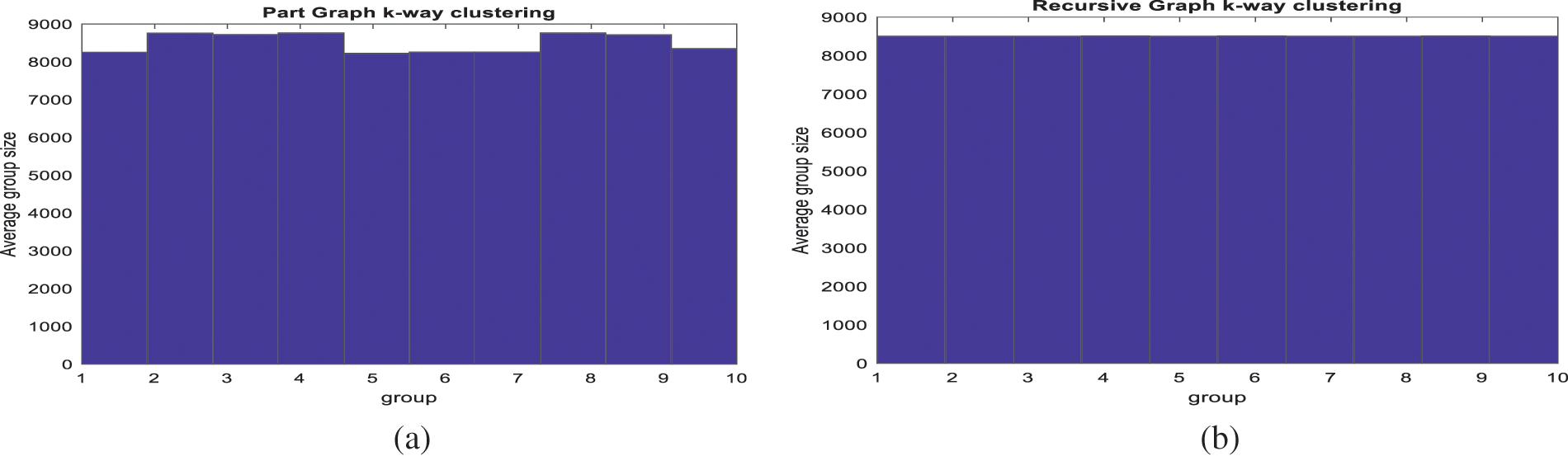
Figure 2: Behance data clustering into similar groups by (a) multilevel k way portioning scheme (b) Multilevel recursive bisection scheme

Entropy considered is the mean of each cluster’s entropy. The entropy grows with the number of groups due to homogeneous division of data. We hereby select 10 clusters for further tensor factorization for the tradeoff between homogeneity and computational cost.

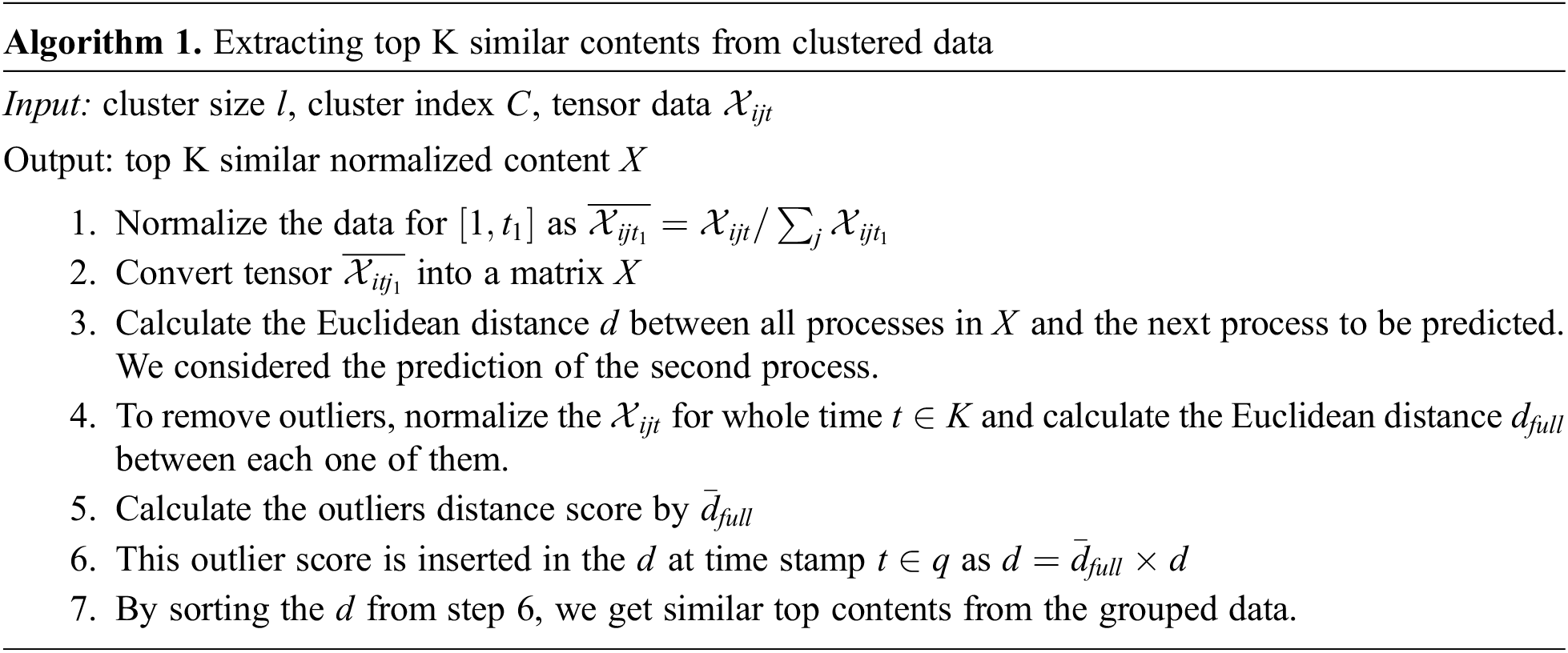
The tensor data of the Behance is huge and it is computationally expensive and less accurate to process this data further for tensor decomposition. We take out similar data to process from the above groups. To extract the similar top contents, we normalized the data for the time period [1,t1] . This way, outliers can be easily extracted and data would be uniform. The distance between each value lies in between [0,1] after normalization, that’s why the whole data in a group won’t differ much in value. The pseudo-code for top k similar contents from Behance tensor data Xijt (see Fig. 3) is given in algorithm 1.

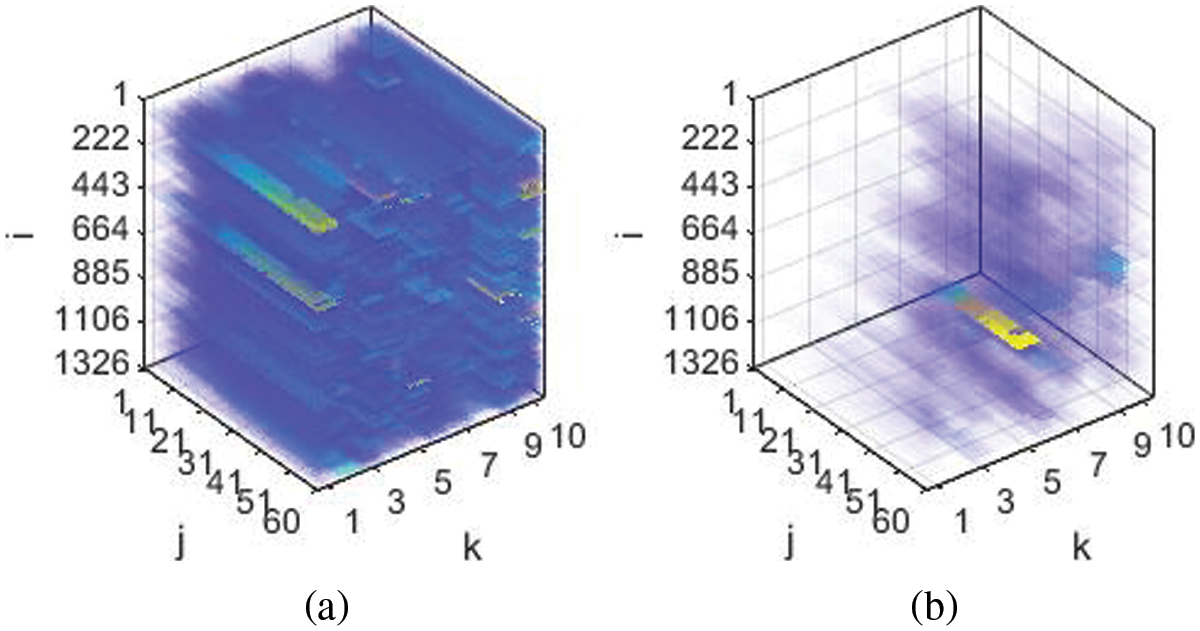
Figure 3: (a) Original Behance data and (b) normalized top K similar grouped contents. The color scheme here represents the magnitude. After normalization, the magnitude variation in data is least and grouped

4  Popularity Prediction by A-PARAFAC

This section is divided into two main subsections. First, we will discuss the augmented PARAFAC for the tensor factorization, then that A-PARFAC will be extended to solve the popularity prediction problem with tensors. Section 4.1 presented the factorization method for the single tensor, but in the work of group-level popularity prediction, the data is divided into four tensors each for group-level, population level for the time (0,t1] (known popularity) and prediction time interval (t1,q] (unknown popularity values). Eq. (6) in Section 4.1 is extended for multiple tensors in Section 4.2.

4.1 A-PARAFAC

As previously stated, the PARAFAC constitutes the platform for the advanced tensor factorization for popularity prediction in our work. The third-order tensor XϵRI×J×K is decomposed into rank 1. The tensor can be recovered from the cross-product of its factors as in Eq. (1) [22,26].

Xitj≈[[D,J,F]]itj:=∑r=1RDirJtrFjr (1)

The recovered tensor is not exactly the same as the original and always has some residual error. So, the decomposition should have minimum error for the case of popularity prediction. This also motivates the idea of data imputation and data prediction can be considered as the subcase of data imputation. So, Eq. (1) can be decomposed to the lowest rank as:

L(X;D,J,F)=12‖X−[[D,J,F]],‖F2 (2)

Here ||.||F is the Frobenius norm. This term on the left-hand side in Eq. (2) should be minimized minD,J,FL(X;D,J,F) and it’s a non-convex optimization problem. The solutions of Eq. (2) trap into local minima due to non-uniform scaling [26]. So, the Tikhonov regularization factor is added into Eq. (2) [28] and updated as

LP(X;D,J,F)=12‖X−[D,J,F]‖F2 + λ2(‖D‖F2 + ‖J‖F2 + ‖F‖F2) (3)

where λ is a regulation parameter with λ>1 , we used the Behance project website data collection for our research [2]. Users upload their work to the site, and visitors may express their appreciation for it by pressing the applaud button. Users, contents, and associated ratings are all part of this tensor data. Eq. (3) transfers that information to the latent space. The future popularity may be less accurate if the temporal dependence on the rating isn’t considered. When a project’s content is above average, a user typically enjoys it. However, people may become less fascinated by the project over time and stop appreciating projects with simply above-average content. Because of their newfound insight, the project’s future popularity is likely to suffer as a result. Some external variables (such as those mentioned in clustering) might affect the project’s fortunes, making it more popular or less popular. We term this shift in project evaluations over time due to variables impacting users or the project’s substance as “biasing”. This biasing is included in Eq. (3). The PARAFAC factorization is referred to as augmented PARAFAC in this case.

LA(X;D,J,F)=12‖X−μ−∅D−θJ−ηF−[D,J,F]‖F2+λ2(‖D‖F2+‖J‖F2+‖F‖F2+‖∅D‖F2+‖θJ‖F2+‖ηF‖F2) (4)

This can be further simplified as

LA(X;D,J,F)=12(‖χ‖F2+‖μ‖F2+‖ϕD‖F2+‖θJ‖F2+‖ηF‖F2+‖[D,J,F]‖F2)−⟨(χ,μ)⟩−⟨(χ,ϕD)⟩−⟨(χ,θJ)⟩−⟨(χ,ηF)⟩−⟨(χ,[D,J,F])⟩+⟨(μ,ϕD)⟩+⟨(μ,θJ)⟩+⟨(μ,ηF)⟩+⟨(μ,[D,J,F])⟩+⟨(ϕD,θJ)⟩+⟨(ϕD,ηF)⟩+⟨(ϕD,[D,J,F])⟩+⟨(θJ,ηF)⟩+⟨(θJ,[D,J,F])⟩+⟨(ηF,[D,J,F])⟩+λ2(‖D‖F2+‖J‖F2+‖F‖F2+‖∅D‖F2+‖θJ‖F2+‖ηF‖F2) (5)

Where ∅D , θJ , ηF are the bias factors for the users and project contents, μ is the mean of all three factors [28]. The bias is calculated as the difference from the mean μ . The decomposed tensor X is shown in Fig. 4. The recovered tensor X^ from the new factors can be represented as X^i,j,t=μ+∅D+θJ+ηF+[D,J,F] .

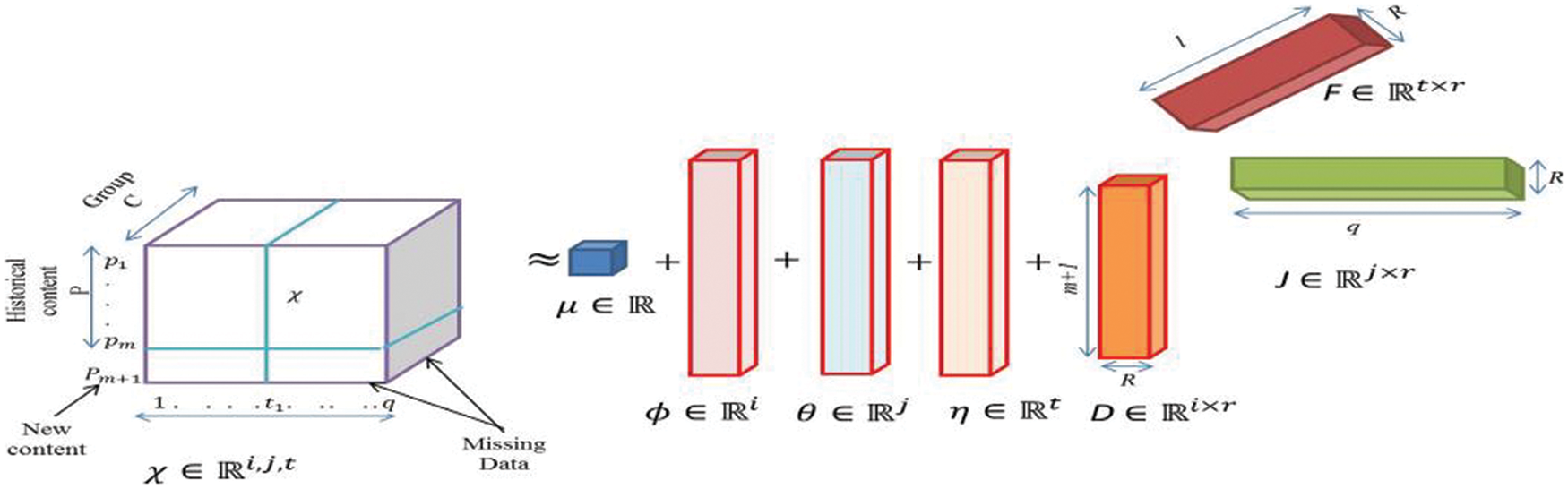
Figure 4: New augmented PARAFAC factorization for 3rd order tensor

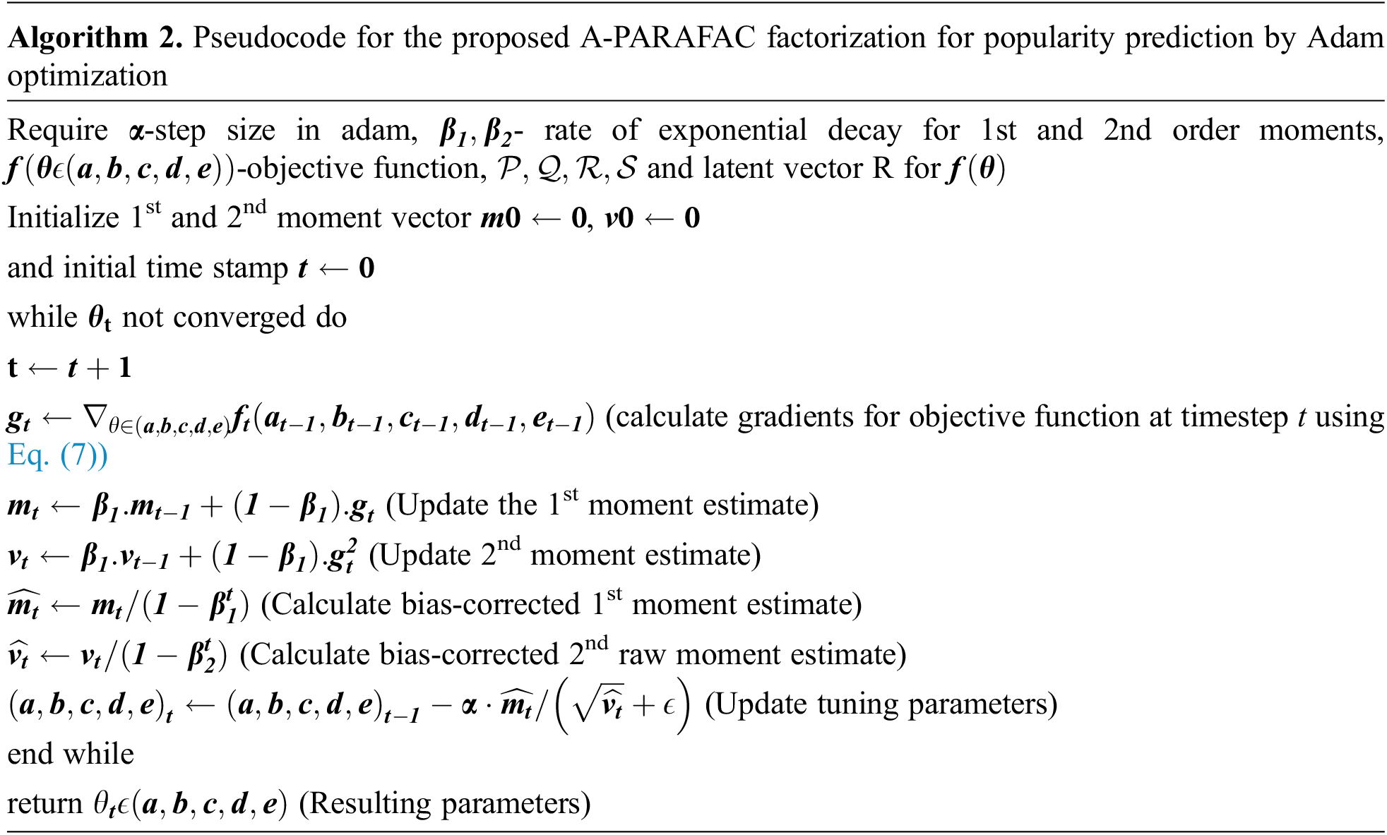
Eq. (5) has been reduced using gradient descent optimization [2] and the Alternating least square technique [24] recently. The downside to these approaches is that they are prone to becoming trapped in local minima with a slow convergence rate. The deep learning schemes in popularity prediction are advanced by Adam optimization [36]. It inspires the replacement of gradient descent and alternating least square optimization algorithms. Eq. (5) is termed as the objective function for the Adam optimization. The bias also varies with the exponential decay function in each iteration of optimization. The bias values may get trapped at an unstable point during the iterations, destabilizing the prediction system. The logistic map can achieve stability analysis concerning bias values. Bias values are updated as in Eq. (6).

∅D,t=∅D,t−1+(Xitj−X^i,j,t)∗xn∗e−αtT (6)

Here (Xitj−X^i,j,t) is the error between the original and reconstructed tensor, α is a constant with a fixed value of 20. t and T represent the current and maximum iteration, respectively. xn is calculated by logistic mapping and a saddle value for stability. It can be calculated as

xn=rxn(1−xn) (7)

The r is a system parameter whose value lies between (0,4]andxnε[0,1] .

4.2 A-PARAFAC in Popularity Prediction

From the clustering step in section III, we get the groups C=C1,C2,C3….Cl which can create a group-level popularity tensor Xijt for the P∪{pm+1} , which are further factorized into D,J,F as shown in Fig. 4. The entries at Xm+1,t,j are missing and need to fill these missing values to predict the popularity pm+1 . The suggested A-PARAFAC tensor factorization does that job for us. The factor matrix Dis for the contents in P∪{pm+1} , matrix J is for t1 time stamps and F represents the latent dimensions.

The tensor vector X can be large and computationally expensive, so we only selected the first k similar tensors and similarity is evaluated by Euclidean distance. Lesser is the Euclidean distance, and more similar is the tensor. Before predicting the pm+1 content, it is normalized for time [1,t1] to standardize the data as in Eq. (8).

Xitj¯=Xitj∑Xitj (8)

We divide the normalized top k-similar data into four tensors P,Q,R,S . P and Q contain the group-level and population level popularity contents in Pg and Pa respectively, R and S contain the popular content of new pm+1 in the time interval (0,t1) . The tensor P contains the content as shown in Fig. 4 with a three-degree tensor ( PεRk×q×l ; k for content, q for the time period and l for groups). Since Q is for population level content only, so a single group is considered as QεRk×q×1 . The R is the group-level content for new content only, so for the time period (0,t1) : RεR1×t1×l and population level content pm+1 for (0,t1] : SεR1×t1×1 . We need to predict the popularity of pm+1 in the interval (t1,q ]. Fig. 5 shows the P,Q,R,S plot after factorization, which is discussed further. The 3D plot in Fig. 5a shows that most of group-level content has higher values at later time stamps and lying around k=5 . It could be different for other data. Hinton diagram in Figs. 5b–5d are of a single color, which is due to the single polarity of values and the size of bars in the diagram denotes the magnitudes of contents.

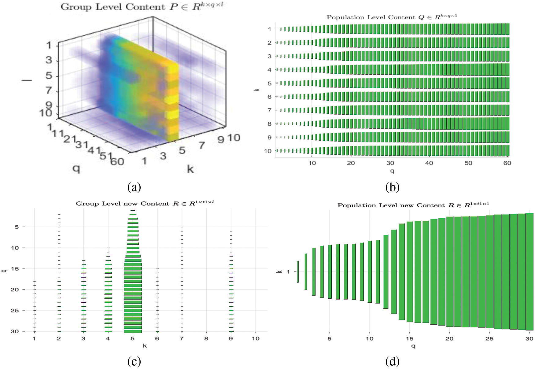
Figure 5: (a) 3D tensor plot for P , Hinton diagram for (b) Q , (c) R (d) S

These four tensors are further factorized as specified in Section 4.1. Fig. 6 shows the visualization of these four tensor factorizations. The P and Q have equal timestamps for J, which is later specified as 30 for training as data has 60 timestamps in total. In R and S , the J will have the other 30 time stamps. Since Q and R predict the population level and group-level popularity for (t1,q] , so the factor in this dimension will be common for both, which is K . Likewise, P and R share the common groups, the factor F will be common in these two tensors. This way, we need to extract the 5 factors out of four tensors. By the clustering scheme, the projects are grouped and J represents the project groups in these notations.

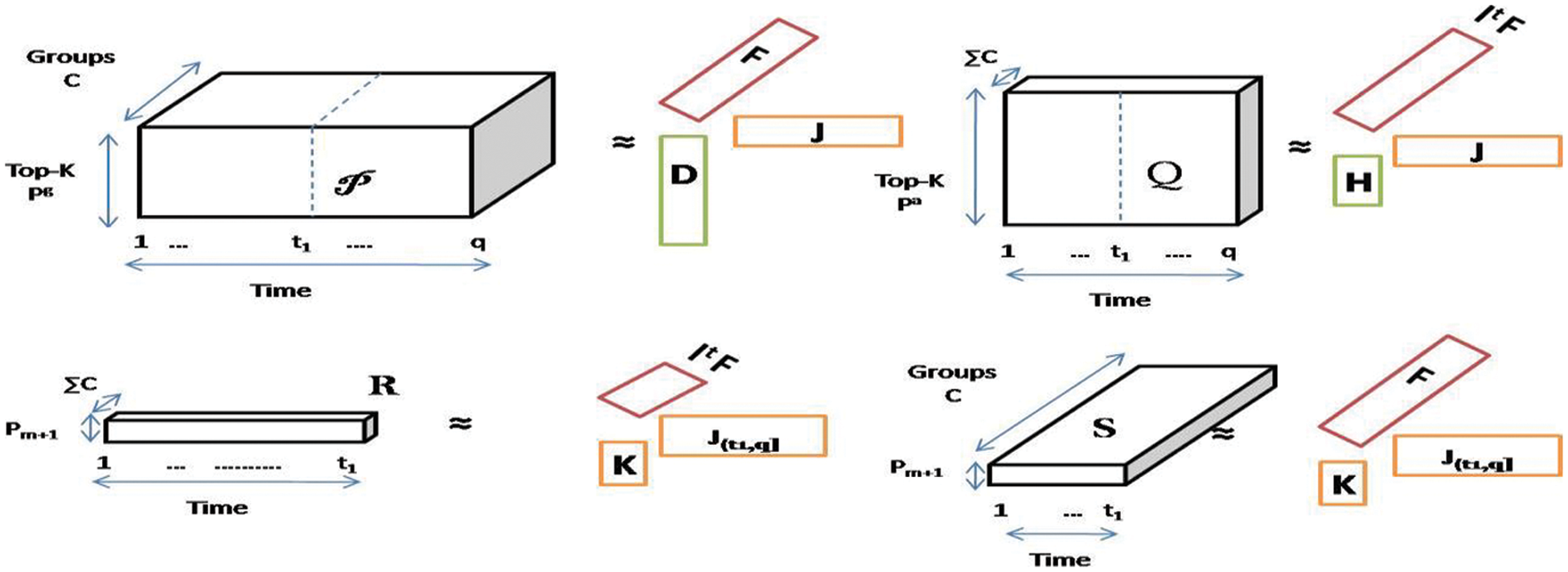
Figure 6: Four tensors’ factorization into three factors where J , K , F are common amongst these tensors

These four tensors are further factorized using Adam optimization into five factors as:

D∈Rk×R,JεRq×R,KεRl×R,HεRk×R,F∈R1×R

After the factorization, the Pg and Pa contents are in the rows of D and J , l user groups with latent dimension R is in factor K , factor H has the timestamps in its rows and F has the single-dimensional content pm+1 . These are converted into tensors instead of the matrix due to the tensor’s faster computation capability. To predict the pm+1 for (t1,q] , only K , F and last (0,t1] rows of H are used. These five factors constitute the above four tensors as:

P≈[[DJF]];Q≈[[H,J,1→TF]];R≈[[K,MTJ,F]];S≈[[K,MTJ,1→TF]] (9)

To predict the popularity, these five factors are decomposed from P,Q,R,S and Eq. (5) is modified for multiple tensors as:

LA(X;D,H,K,J,F)=12‖X−X^i,j,t,1‖F2+12‖X−X^i,j,t,2‖F2+12‖X−X^i,j,t,3‖F2+12‖X−X^i,j,t,4‖F2+12‖X−X^i,j,t,5‖F2+λ2(‖D‖F2+‖H‖F2+‖K‖F2+‖J‖F2+‖F‖F2+‖∅D‖F2+‖θJ‖F2+‖ηF‖F2) (10)

where each tensor hat is the sum of mean, biases and factors of tensor as:

X^i,j,t,1=μ+∅D+θJ+ηF+[D,J,F] (11)

X^i,j,t,2=μ+∅D+θJ+ηF+[H,J,1→TF] (12)

X^i,j,t,3=μ+∅D+θJ+ηF+[K,MTJ,F] (13)

X^i,j,t,4=μ+∅D+θJ+ηF+[K,MTJ,1→TF] (14)

The tensor factorization for popularity prediction for pm+1 content by A-PARAFAC scheme is given in algorithm 2. Eq. (10) is minimized through adam optimization method. This stochastic optimization requires gradients to be calculated [6]. To calculate the gradients, the partial derivative of Eq. (11) is taken w.r.t. D,H,K,J,F . For example, the partial derivative of the above equation w.r.t. D is represented in Eq. (16). Bias terms are constant, so they will be neglected. To get the gradient, the square of Frobenius norm is solved by algebraic formulation (a+b)2 . We elaborate the solution for the first term in Eq. (11) and the rest will follow a similar solution.

‖X−X^i,j,t,1‖F2=‖X−μ+∅D+θJ+ηF+[D,J,F]‖F2...using (15)

Eq. (12)

Since [D,J,F] are factors of tensor and a tensor can be composed of the cross product of factors, so the gradient of this term will result in J⊙F .

∇DLA=−(X−X^i,j,t,1)(J⊙F)+λD (16)

Similarly, other derivatives are;

∇HLA=−(X−X^i,j,t,2)(J⊙1→TF)+λH (17)

∇KLA=−(X−X^i,j,t,3)(MTJ⊙F)+λK−(X−X^i,j,t,4)(MTJ⊙1→TF) (18)

∇JLA=−(X−X^i,j,t,1)(F⊙D)−(X−X^i,j,t,2)(H⊙1→TF)−M(X−X^i,j,t,3)(K⊙F)−M(X−X^i,j,t,4)(1→TF⊙K)+λJ (19)

∇FLA=−(X−X^i,j,t,1)(J⊙D)−(X−X^i,j,t,2)(H⊙J)−M(X−X^i,j,t,3)(K⊙MTJ)−M(X−X^i,j,t,4)(MTJ⊙K)+λF (20)

5  Experiments

In this section, we comparatively evaluated the proposed prediction scheme on real world datasets. In real-world datasets, we used Behance dataset [2]. The proposed algorithm is tested on the hardware with an Intel core with a frequency of 2.20 GHz, 12 GB RAM, 2 GB Nvidia graphics.

5.1 Baselines

Social media popularity prediction is an interesting field for other researchers too. We will compare our work with other states of the art in this field. The latest work based on grouping and conventional PARFAC tensor factorization is done by Hoang et al. [2]. They used the gradient descent (GD) algorithm to factorize the tensor and predict the popularity but the GD suffers from slow convergence and local minima problem. Adam optimization is a better alternative for that. Further, we tested the collaborative filtering based prediction methods on dataset [6,7,37]. These methods used user based tensor factorization while [7] blended the factorization method with a neighborhood scheme. Its approach is at the population level, whereas [6,37] is predicted at the user level. We used user level and population popularity prediction as population level gives a coarser view while vice versa is for user level prediction.

5.2 Experimental Setup

We have used the Behance dataset which is extracted from Behance API for 60 days. 30-time stamps are used for prediction for the testing. The regularization factor and latent dimension used in it are 0.1 and 50, respectively. The bias update constant factor α is taken as 20, while the total iterations T is 300. Data is divided into ten groups as discussed in Section 3. We evaluated the work by the relative error percentage (REP) parameter. It is calculated as:

REP=∑i,t>t−1|∑jXitj−∑jX^itj∑i,t>t1,jXitj×100% (21)

Here X^itj is the predicted tensor.

To test the proposed model, dataset is obtained from Behance network [2]. The dataset of 85092 users for 1326 projects for timestamps of 60 h was gathered in June 2014. Due to this large size dataset, we need to select the top k similar contents.

5.3 Prediction Analysis

We tested the A-PARAFAC with modified adam optimization for tensor factorization. The factors K∈Rl×R,J∈Rk×R,F∈R1×R;k∈[t1+1,t2] thus formed are recombined in a tensor. This reconstructed tensor is the predicted data for the time stamp t1+1<q<t2 . The biases calculated from eq. (8) are directly related to prediction error. We have predicted the popularity for 30 days for the Behance data. Fig. 7 shows the predicted rating plot for each cluster for 30 days. Figs. 7a and 7b has more homogeneous clusters than 9(c), (d), as discussed in Section 3. The 5th cluster by the proposed clustering scheme has a highly popular project, while with the part graph scheme, it is assigned to 4th cluster. Analysis of Fig. 7 shows that the predicted popularity of clusters 1, 2, 9, 10 differs more in the previous method with gradient descent [2], whereas these are more similar to ground truth by the proposed scheme.

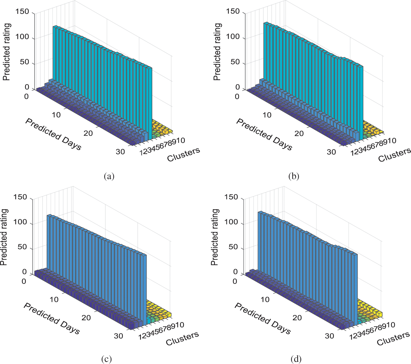
Figure 7: Plot for predicted popularity for Behance data (a) popularity calculated by A-PARAFAC for the recursively k-way grouped contents (b) ground truth project ratings for the time period [ t1+1,t2 ] (c) popularity calculation by part graph k-way clustering with gradient descent optimization (d) ground truth popularity by the part graph grouped data

We also compared the proposed algorithm with other variants too, as in Tab. 1. Our work has two stages of the algorithm: clustering of data and selecting top k similar, Tensor factorization. Analysis of Tab. 1 suggests that the grouping method is the key factor for better accuracy. As clustering removes outliers and deals with the change in the project rating due to external conditions. The A-PARAFAC, with its data noise (change in user’s nature with time to judge the project at Behance) immunity strength, performs best with Multilevel recursive group-based (MRGB) clustering. Another work on group level popularity is presented in an article by Hoang et al. [2]. This work clustered the data by K-level partitioning, which makes the less homogeneous clusters than MRGB, as discussed in Section 3. The MRGB clustering has gained an improvement of 5.6%, which is listed in Tab. 1 with the name MRGB+GD. We change the gradient descent optimization method by Adam and an improvement of 11.11% than with k-level partitioning+GD is witnessed. The PARAFAC decomposition is improved by adding biases and regularization parameters. This A-PARAFAC is evaluated with the k-level partitioning and MRGB clustering, respectively. The optimization used is Adam in both experiments. It is worth mentioning that the k-level clustered with the proposed A-PARAFAC has touched the gain of 19.09% than k-level+PARAFAC+Adam prediction error and 20.39% than the work by Hoang et al. [2].

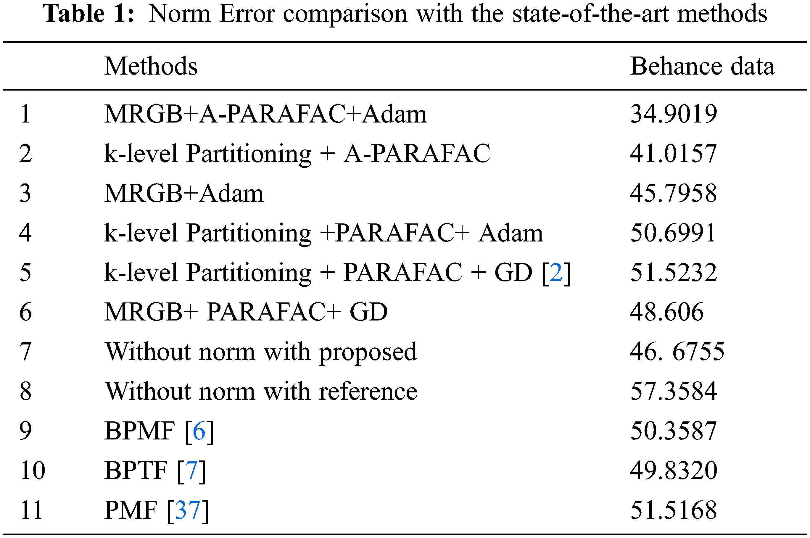
The proposed MRGB clustered A-PARAFAC with Adam optimization has minimized the prediction norm error to 34.9019 which is the lowest among all variants and improved the accuracy by 32.25% to the baseline method. Besides the group-level baseline comparison, we also test the norm error readings with a few user-level prediction schemes. The first method in this queue has made use of probabilistic matrix factorization (PMF) [37,38]. The PMF is a variant of non-negative matrix factorization (NMF). The NMF is the backbone of autoencoders in deep learning. In PMF Mnih et al. [37] added the regularization parameters for two decomposed factors of a matrix. The authors have shared their MATLAB code publicly and a small tweak in the code makes it feasible to test it on our dataset. 20.38% is the improvement of our proposed scheme from the error in PMF prediction. Salakhutdinov et al. [6] worked on enhancing the PMF prediction. They added the Bayesian treatment to all hyperparameters in the regularization terms of PMF and tuned these parameters by Markov chain Monte Carlo method. The test of this method with our dataset shows an improvement of 2.29% than PMF but 30.69% more errors than our proposed prediction scheme. Further, the authors in [7] introduced the automatic rank determination in the Bayesian factorization scheme. The results have shown an improvement than [6] and [37]; however, the norm error in the prediction is 29.96% more than the MRGB clustered-Adam optimized A-PARAFAC.

In our previous work [39], we used adam optimization with conventional PARAFC factorization to improve the prediction. Since Eq. (11) is for advanced-PARAFAC, the solution of this with biases lower the value than PARAFAC with Adam. Fig. 8 also shows the comparison for popularity prediction error plot for gradient descent optimization of PARAFC, Adam optimization of PARAFAC, and Updated Adam optimization for A-PARAFAC. Since biases are chaotically updated with normalized prediction error, these have similar values and scale. Since the prediction error is perturbed by logistic mapping and added to the previous bias in each iteration, the bias value increases, whereas the error decreases in the same fashion (Fig. 8).

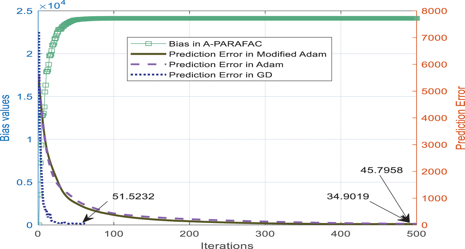
Figure 8: Comparison plot for normalized popularity prediction error at each iteration of the optimization

6  Conclusion

We developed a new method for predicting the popularity of tensor groups on social media. The tensor data is grouped and factorised to the lowest rank in order to estimate the level of participation in the future. This paper examines two well-known tree-based hierarchical clustering algorithms: partway k-level clustering and multilevel recursive clustering. The latter’s uniformity pertains more to our research. As the number of clusters grows, so does the degree of group homogeneity, therefore, we run the experiment with ten clusters. Changes in user criteria for rating projects in the future have necessitated an upgrade to standard PARAFC tensor factorization algorithm. There are three biases introduced to the PARAFAC factors since our tensor data is formatted in a three-way manner for users, projects, and their ratings. As a result of this modification, the prediction accuracy is now 32.25% higher than it was previously [2]. Clustering and tensor factorization algorithms were also used in additional test scenarios. Before, PARAFAC employed the gradient descent approach. The newest Adam optimization was substituted, and we were able to generate seven distinct test cases as a result. A-PARAFAC, the suggested method for MRGB prediction, offers the best accuracy.

Graph-level deep learning techniques (generative or structural) can be used in conjunction with a bespoke database to enhance this work. To ensure that the suggested solution works, real-time testing may be carried out in order to verify it.

Acknowledgement: We would like to thanks management of Maharaja Surajmal Institute of Technology, New Delhi and NSUT, East Campus (Formerly AIACTR), New Delhi for providing support to carry out this research.

Funding Statement: The authors received no specific funding for this study.

Conflicts of Interest: The authors declare that they have no conflicts of interest to report regarding the present study.

References

1. B. Wu, W. H. Cheng, Y. Zhang, Q. Huang, J. Li et al., “Sequential prediction of social media popularity with deep temporal context networks,” in Proc. IJCAI, Melbourne, Australia, pp. 3062–3068, 2017. [Google Scholar]
2. M. X. Hoang, X. H. Dang, X. Wu, Z. Yan and A. K. Singh, “GPOP: Scalable group-level popularity prediction for online content in social networks,” in Proc. WWW, Perth, Australia, pp. 725–733, 2017. [Google Scholar]
3. Y. Hu, C. Hu, S. Fu, P. Shi and B. Ning, “Predicting the popularity of viral topics based on time series forecasting,” Neurocomputing, vol. 210, pp. 55–65, 2016. [Google Scholar]
4. S. Moro, P. Rita and B. Vala, “Predicting social media performance metrics and evaluation of the impact on brand building: A data mining approach,” Journal of Business Research, vol. 69, no. 9, pp. 1–11, 2016. [Google Scholar]
5. K. Fernandes, P. Vinagre and P. Cortez, “A proactive intelligent decision support system for predicting the popularity of online news,” in Proc. EPIA, Coimbra, Portugal, vol.9273, pp. 535–546, 2015. [Google Scholar]
6. R. Salakhutdinov and A. Mnih, “Bayesian probabilistic matrix factorization using Markov chain Monte Carlo,” in Proc.ICML, Helsinki, Finland, pp. 880–887, 2008. [Google Scholar]
7. L. Xiong, X. Chen, T. Huang, J. Schneider and J. G. Carbonell, “Temporal collaborative filtering with Bayesian probabilistic tensor factorization,” in Proc. SDM, Columbus, Ohio, pp. 211–222, 2010. [Google Scholar]
8. T. G. Kolda and B. W. Bader, “Tensor decompositions and applications,” SIAM Review, vol. 51, no. 3, pp. 455–500, 2009. [Google Scholar]
9. G. Karypis and V. Kumar, “Parallel multilevel k-way partitioning scheme for irregular graphs,” in Proc. Supercomputing, Pittsburgh, PA, USA, pp. 35–35, 1996. [Google Scholar]
10. Y. Chen, C. Hsu and H. M. Liao, “Simultaneous tensor decomposition and completion using factor priors,” IEEE Transactions on Pattern Analysis and Machine Intelligence, vol. 36, no. 3, pp. 577–591, 2014. [Google Scholar]
11. D. Goldfarb and Z. Qin, “Robust low-rank tensor recovery: Models and algorithms,” SIAM Journal on Matrix Analysis and Applications, vol. 35, no. 1, pp. 225–253, 2014. [Google Scholar]
12. T. Maehara, K. Hayashi and K. Kawarabayashi, “Expected tensor decomposition with stochastic gradient descent,” in Proc. AAAI, Phoenix, Arizona, USA, pp. 1919–1925, 2016. [Google Scholar]
13. S. De, A. Maity, V. Goel, S. Shitole and A. Bhattacharya, “Predicting the popularity of Instagram posts for a lifestyle magazine using deep learning,” in Proc. CSCITA, Mumbai, pp. 174–177, 2017. [Google Scholar]
14. S. Das, B. V. Syiem and H. K. Kalita, “Popularity analysis on social network: A big data analysis,” in Proc. CCSN, Odisha, India, pp. 27–31, 2014. [Google Scholar]
15. S. Stieglitz, M. Mirbabaie, B. Ross and C. Neuberger, “Social media analytics – challenges in topic discovery, data collection, and data preparation,” International Journal of Information Management, vol. 39, pp. 156–168, 2018. [Google Scholar]
16. S. V. Canneyt, P. Leroux, B. Dhoedt and T. Demeester, “Modeling and predicting the popularity of online news based on temporal and content-related features,” Multimedia Tools and Applications, vol. 77, no. 1, pp. 1409–1436, 2017. [Google Scholar]
17. M. T. Uddin, M. J. A. Patwary, T. Ahsan and M. S. Alam, “Predicting the popularity of online news from content metadata,” in Proc. ICISET, Dhaka, pp. 1–5, 2016. [Google Scholar]
18. S. Aghababaei and M. Makrehchi, “Mining social media content for crime prediction,” in Proc. WI, Omaha, NE, USA, pp. 526–531, 2016. [Google Scholar]
19. E. S. Allman, P. D. Jarvis, J. A. Rhodes and J. G. Sumner, “Tensor rank, invariants, inequalities, and applications,” SIAM Journal on Matrix Analysis and Applications, vol. 34, no. 3, pp. 1014–1045, 2013. [Google Scholar]
20. C. J. Hillar and L. H. Lim, “Most tensor problems are NP-hard,” Journal of the ACM, vol. 60, no. 6, pp. 1–39, 2013. [Google Scholar]
21. P. Paatero, “Construction and analysis of degenerate PARAFAC models,” Journal of Chemometrics: A Journal of the Chemometrics Society, vol. 14, no. 3, pp. 285–299, 2000. [Google Scholar]
22. X. Chen, Z. He, Y. Chen, Y. Lu and J. Wang, “Missing traffic data imputation and pattern discovery with a Bayesian augmented tensor factorization model,” Transportation Research Part C: Emerging Technologies, vol. 104, pp. 66–77, 2019. [Google Scholar]
23. X. Chen, Z. He and J. Wang, “Spatial-temporal traffic speed patterns discovery and incomplete data recovery via SVD-combined tensor decomposition,” Transportation Research Part C: Emerging Technologies, vol. 86, pp. 59–77, 2018. [Google Scholar]
24. Y. Koren, R. Bell and C. Volinsky, “Matrix factorization techniques for recommender systems,” Computer, vol. 8, no. 8, pp. 30–37, 2009. [Google Scholar]
25. J. Charlier and V. Makarenkov, “VecHGrad for solving accurately complex tensor decomposition,” arXiv preprint arXiv: 1905.12413, 2019. [Google Scholar]
26. Y. Koren, “Collaborative filtering with temporal dynamics,” in Proc. KDD, Paris, France, pp. 447–456, 2009. [Google Scholar]
27. Y. Hu, Y. Koren and C. Volinsky, “Collaborative filtering for implicit feedback datasets,” in Proc. ICDM, Pisa, Italy, pp. 263–272, 2008. [Google Scholar]
28. N. Joseph, A. Sultan, A. K. Kar and P. Vigneswara Ilavarasan, “Machine learning approach to analyze and predict the popularity of tweets with images,” in Proc. I3E, Kuwait City, Kuwait, pp. 567–576, 2018. [Google Scholar]
29. H. Sun and R. Grishman, “Employing lexicalized dependency paths for active learning of relation extraction,” Intelligent Automation & Soft Computing, vol. 34, no. 3, pp. 1415–1423, 2022. [Google Scholar]
30. H. Sun and R. Grishman, “Lexicalized dependency paths based supervised learning for relation extraction,” Computer Systems Science and Engineering, vol. 43, no. 3, pp. 861–870, 2022. [Google Scholar]
31. R. Aswani, S. Chandra, S. P. Ghrera and A. K. Kar, “Identifying popular online news: An approach using chaotic cuckoo search algorithm,” in Proc. CSITSS, Bengaluru, India, pp. 1–6, 2017. [Google Scholar]
32. R. Aswani, A. K. Kar, S. Aggarwal and P. Vigneswara Ilavarsan, “Exploring content virality in Facebook: A semantic based approach,” in Proc. I3E, Swansea, United Kingdom, pp. 209–220, 2017. [Google Scholar]
33. Q. Cao, H. W. Shen, H. Gao, J. Gao and X. Cheng, “Predicting the popularity of online content with group-specific models,” in Proc. WWW, Perth, Australia, pp. 765–766, 2017. [Google Scholar]
34. Q. Cao, H. Shen, K. Cen, W. Ouyang and X. Cheng, “Deephawkes: bridging the gap between prediction and understanding of information cascades,” in Proc. CIKM, Singapore, pp. 1149–1158, 2017. [Google Scholar]
35. S. T. Barnard, “PMRSB: Parallel multilevel recursive spectral bisection,” in Proc. Supercomputing, San Diego, CA, USA, pp. 27–27, 1995. [Google Scholar]
36. D. P. Kingma and J. Ba, “Adam: A method for stochastic optimization,” in Proc. ICLR, San Diego, CA, USA, pp. 1–15, 2015. [Google Scholar]
37. A. Mnih and R. Salakhutdinov, “Probabilistic matrix factorization,” in Proc. NIPS, Vancouver British Columbia Canada, pp. 1257–1264, 2008. [Google Scholar]
38. P. Kherwa, S. Ahlawat, R. Sobti, S. Mathur and G. Mohan, “Predicting socio-economic features for indian states using satellite imagery,” in Proc. ICICC, New Delhi, vol.1166, pp. 497–5082021 [Google Scholar]
39. N. Bohra and V. Bhatnagar, “Group level social media popularity prediction by MRGB and Adam optimization,” Journal of Combinatorial Optimization, vol. 41, no. 2, pp. 328–347, 2021. [Google Scholar]
Cite This Article
Copyright © 2023 The Author(s). Published by Tech Science Press.
This work is licensed under a Creative Commons Attribution 4.0 International License , which permits unrestricted use, distribution, and reproduction in any medium, provided the original work is properly cited.
Downloads
Citation Tools