Automatic Image Annotation Using Adaptive Convolutional Deep Learning Model

1  Introduction

With innovative progress, it is gradually becoming more direct that individuals take photos in different areas and exercises. There are thousands of personal photos if not millions. Accordingly, taking care of searched photos has become a boring and difficult task. Image rendering technique (image concept) involves assigning at least one name (labels) to an image depicting its subject. This method can be used for a variety of mistakes, including planned photo naming through online entertainment, planned photo imagery for outsiders, and programmed text creation from images [1].

Recently, as the number of images has been growing, individuals need to use image concept to view a greater number of images and monitor productivity [2]. In the field of application, today’s devices and gear are of significant importance for the planned arrangement of the image segment. This can give the specialist the determination of the patient’s disease. The order and section of the image are within the scope of the image concept [3]. It is necessary to initially order pixels or super pixels to separate the images well. Then it creates a sense for the assorted area of the pixels, which is really what the image segment wants to get. In this way, order is paramount during clinical picture commentary [4]. Therefore, in recent years, many researchers in this field have made relentless efforts to further improve the accuracy of the sequence, although the characterization of the images concept problem is indeed critical of many problems and difficulties [5].

Deep learning calculations are generally intended to fall within the realm of man-made reasoning and to obtain clear information. Deep learning models require enormous, varied product datasets for better modeling [6]. The ImageNet database is used to produce robust wide-ranging effective deep learning image assortments, each of which contains a number of notable images that are used to illustrate the articles in the image [7]. Although generally very modest, the datasets used to produce robust medical image classifiers contain hundreds to thousands of charts. The task expected of organizing these product databases is widely seen as a significant obstacle to the progress of the deep learning framework.

Various programming tools have been developed to comment on imaging. These tools typically name manual, semi-robotic, and fully computerized techniques for imaging. Semi-automated techniques typically use conventional image manipulation procedures [8], for example, thresholding or edge recognition. Fully automated techniques are generally based on semi-robotic procedures and man-made calculations that encrypt space explicit information. These calculations are difficult to upgrade and the calculation time associated with running a significant amount of them can be significant [9]. In-depth learning calculations figure out how to identify objects of interest in imaging information. The use of in-depth learning-based approaches to the concept of medical imaging does not require the development of conventional man-made calculations. In general, in-depth learning avenues for manipulating image selection have been found to meet or surpass the exhibition of conventional calculations [10]. The expected calculation time to make guesses using in-depth learning models is often shorter than conventional methods. It proposes that an in-depth learning-based approach to the concept of database may meet or surpass the exhibition of conventional human-planned descriptive calculations

Contribution and organization of the paper

■   In this paper, ACDLM is developed for automatic image annotation. Initially, the databases are collected from the open-source system which consists of some labelled images (for training phase) and some unlabeled images {Corel 5 K, MSRC v2}.

■   After that, the images are sent to the pre-processing step such as colour space quantization and texture color class map. The pre-processed images are sent to the segmentation approach for efficient labelling technique J-image segmentation (JSEG).

■   The final step is an automatic annotation using ACDLM which is a combination of Convolutional Neural Network (CNN) and Honey Badger Algorithm (HBA). Based on the proposed classifier, the unlabeled images are labelled.

■   The proposed methodology is implemented in MATLAB and performances is evaluated by performance metrics such as accuracy, precision, recall and F1_Measure. With the assistance of the proposed methodology, the unlabeled images are labelled.

The remaining portion of the article is pre-planned as follows, Section 2 analysis the review of the research papers of annotations. The projected technique of the projected technique is analyzed in the Section 3. The outcomes of the projected technique are illustrated in the Section 4. The summary of the projected technique is presented in the Section 5.

2  Literature Review

Adnan et al., [11] provided an automated image annotation approach using the Convolutional Neural Network-Slantlet Transform. Its purpose is towards convert an image into single or multiple labels. It is essential to understand the visual content of a film. One of the challenges of image references is the need for vague information to generate semantic-level concepts from the original image pixels. Unlike a text annotation that combines words in a dictionary with their meaning, source image pixels are not sufficient to directly form semantic-level concepts. Based on the syntax with the other hand, the well explained for combined letters towards form word sentences and words.

Mehmood et al., [9] have introduced content-based image recovery and semantic programmed image interpretation in the light natural weight of three-sided histograms using the support vector machine. The proposed approach adds image-spatial meaning to the sad record of the BoVW model, minimizing the problem of over-alignment in large-scale wording, and undeniable semantic hole issues between status image semantics and low-level image highlights.

Niu et al., [12] have introduced a novel multi-dimensional in-depth model for the removal of rich and discriminatory elements relevant to a wide range of visual concepts. In particular, an original two-branch deep neural network engineering was proposed, which included a friend specialization network branch with the aim of intertwining a very deep basic organizational branch and the diverse features derived from the primary branch. The deeper model was converted to multi-modular, complementing the image input, taking the labels given by the turbulent client as a sample contribution. To deal with the next problem, we offer the task of scoring a forecast assistant for the basic name expectation assignment to undoubtedly measure the best name number for a given image.

Philbrick et al., [13] have introduced Contour based model to expedite the concept of medical images, with in-depth learning. A significant objective in motivating product development is to establish a climate that empowers clinically organized clients to use in-depth learning models to quickly clarify medical imaging. This approach explains clinical imaging using fully automated in-depth learning techniques, semi-computerized techniques and manual techniques with vocal and additional text descriptions. To minimize feedback errors, it normalizes image feedback throughout the database. It further accelerates clinical imaging interpretation through feedback through in-depth learning (AID). AID’s hidden idea is to repeatedly clarify, train, and apply in-depth learning models during a sample rotation of database concepts and events. To improve this, it supports work processes in which various image specialists clarify clinical images, radiologists support ideas, and information researchers use these concepts to produce in-depth learning models.

Zhu et al., [14] have introduced a startup to complete the in-depth learning framework for object-level multilabel interpretation of multilabel remote detection images. The proposed system consists of a common convolutional brain network for discriminating component learning, a grouping branch for multilabel interpretation, and an embedded branch for securing visual-level close links. In the grouping branch, a review tool was known for creating attention-grabbing highlights, and skip-layer associations were integrated to integrate data from different layers. The mode of thinking of the injection branch should consist of visual representations of images with similar visual-level semantic ideas. The proposed strategy embraces the parallel cross-entropy misfortune of order and the three misfortunes of learning to insert the image. Sun et al., [15] developed a multifeatured learning model with local and global branches. In order to obtain multi-scale information multi scale pooling is utilized. The approach performed effectively for VehicleID dataset. Karthic et al., [16] designed a hybrid approach with stacked encoder for retrieving relevant features and optimized LSTM for classification purpose. This approach proved to be better than approaches without feature selection.

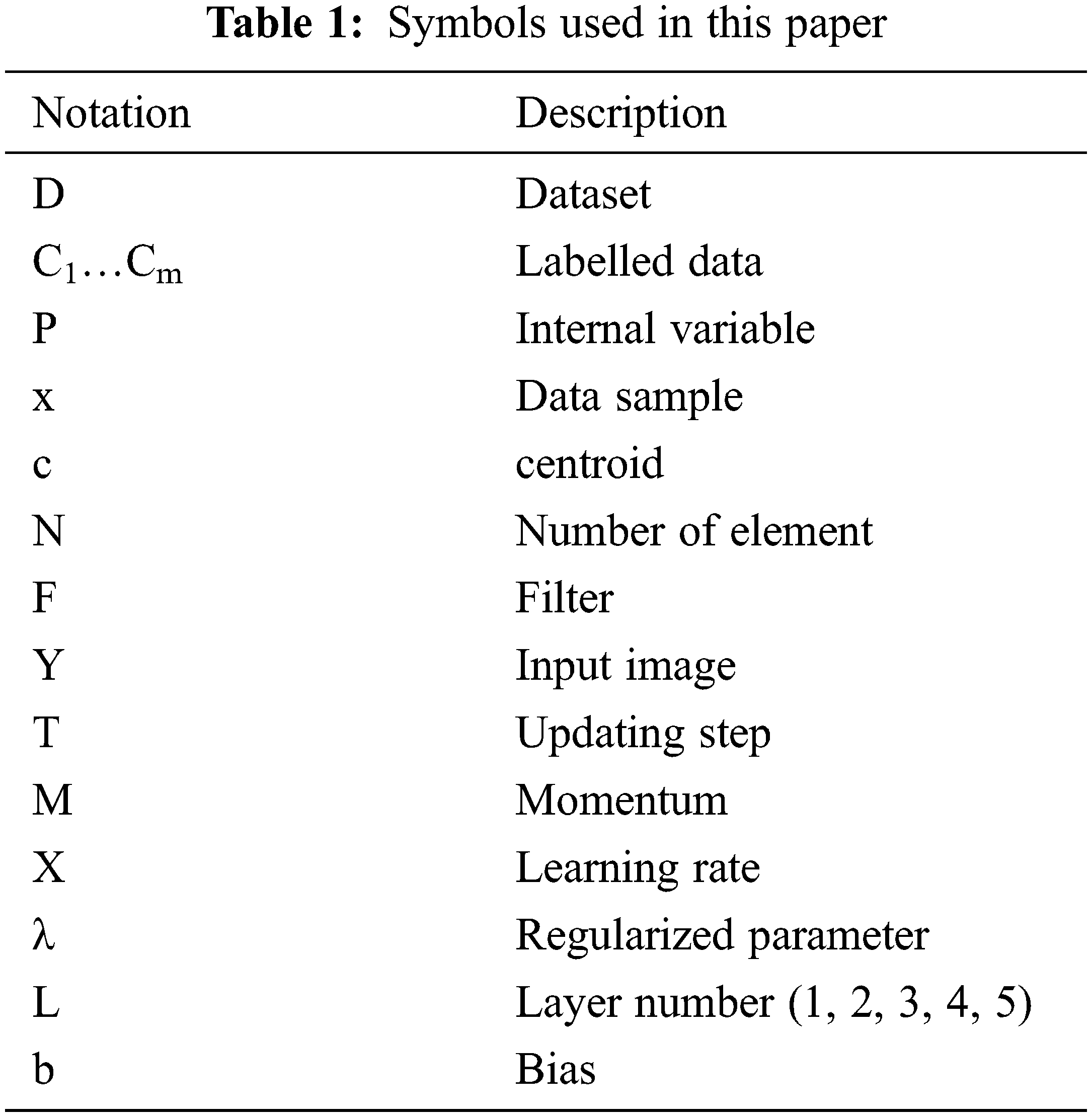
From the literature, lot of image annotation methods had explained. Even though, some improvements are needed in the accuracy. To improve the accuracy, in this paper, novel method is introduced. The notation used in this paper is listed in Tab. 1.

3  Proposed System Model

Traditional annotation techniques are considering the image as holistic through analyzing images globally compared than managing with every presented object. In normal cases, moreover, some theories should give description of the image holistically like wild or joy. Mostly, theories are concerned about few specified locations of the image like cloud, human and football. Based on the outcomes, the conventional techniques achieved efficient outcomes which accounts for visual variations related with regions and semantic interconnections among labels. Presented a theory of region co-occurrence matrix can be computed from an annotated training image set. This projected set provides the similarity from the candidate location and the training subset utilizing the theory of region co-occurrence matrix. With the consideration, the visual correlations with the areas are considered in this technique.

Hence, in this paper, the CNN with HBA is utilized to annotate new regions. Fig. 1 provides the complete structure of projected approach. The projected model is design to achieve image annotations from the images. Initially, the projected approach is containing of image sets D={i1,…,iN} . From the images, few image are labeled and remaining images are not labelled. So, the described every training image, it is labelled with iCN∈CC={C1,…,CM} . The complete images are sent to the pre-processing phase in which they are segmented with the assistance of JSEG technique into visually homogenous areas. The aggregation technique is utilized to reduce the large number of regions through codifying comparable regions into considered as the one label. In this paper, Adaptive Convolutional Deep Learning Model is utilized to label the images. The detail information of the projected technique is explained in the below section.

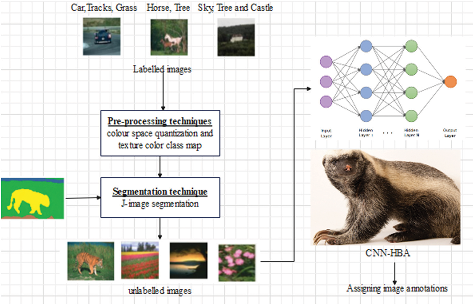
Figure 1: Overall structure of projected approach

3.1 Color Space Quantization

Colour image quantization is a transformation of a true colour image into an image consisting of a smaller number of specially chosen colour. Colour quantization can be utilized as an auxiliary function in colour image processing [17]. In this projected technique, K-harmonic Means Technique (KHM) is developed for image quantization. This formulation is presented as follows,

KHM(x,c)=∑I=1NK∑J=1K1‖XI−CJ‖p (1)

The KHM method needs defining an internal variable P, that normally completes below condition P≥2. Here, we utilize the parameter P = 2.7. The fuzzy membership function of the cluster pixel is applied in addition was compensated by the dynamic weight function, that means varied influence a solitary pixel on computing the novel parameters in upcoming iteration.

M(CJ|XI)=‖XI−CJ‖−P−2∑J=1K⁡‖XI−CJ‖−P−2 (2)

W(XI)=∑J=1K⁡‖XI−CJ‖−P−2(∑J=1K⁡‖XI−CJ‖−P)2 (3)

The KHM approach, based on above formulation, the below formula is utilized for computing novel cluster centers,

CJ=∑I=1N⁡M(CJ|XI)W(XI)XI∑I=1N⁡M(CJ|XI)W(XI) (4)

Based on the quantization approaches are utilized with the similar deterministic initialization technique.

Texture Color Class Map

The quantization is completed in the colour space without describing the spatial variations of the colors. After that, the image pixel parameters are changed through their related color class labels, it forms a class map of the image. The class map is analyzed as a specific kind of texture composition. The colour space quantization and texture color class map is considered as the segmentation phases. The detail segmentation process is explained in the below section.

3.2 Segmentation Stage

In the segmentation process, the J-image segmentation is utilized. Based on the segmentation process, the optimal way to detect objects from an image is to segment them and then extract features from those segmented locations. The object segmentation is a complex method of attaining accurate and precise semantic segmentation. It is achieved on many situations which segmented locations hold presentation annotation of the segmentation quality. JSEG [18] is an efficient segmentation technique for colour images which justified its robustness and effectiveness in a different application. JSEG has normally witnessed different enhancements to enhance its presentations. JSEG technique is developed to perform image segmentation into a set of semantic locations. Initially, the pre-processing stage, the colour space quantization and texture colour map technique are utilized. So, the colour space can be initially quantized and complete pixels of the images are connected with the related bins. In the segmentation stage, the J-image in addition a class map for every windowed colour location can be computed and finally, the clustering approach is utilized to achieve distinct locations. The segmented images are sent to the classification for image annotations. The detail description of the CNN and HBA is given in the below section.

3.3 Convolutional Neural Network

The convolutional neural network can be a specific type of multilevel perceptron design which utilized to human activity recognition from the images. In compare to conventional machine learning techniques, CNN provide spatial data into considered. So, the neighboring pixels can be computed together. The combination of this characterization with the generalization capability of CNN creates them higher to remaining techniques in a number of computer vision submissions. The base parameters of CNN are a convolution layer that operates the convolution operation in the input is an outcome of the upcoming layer [19].

CNN is the efficient generated utilized kind of artificial neural network. Additionally, a CNN is consisting of a multilayer perceptron (MLP). Each solitary neuron in MLP is designed with the activation function which connected with the weighted inputs to the final output. The MLP is designed with the deep MLP and the solitary hidden layer is connected to the network structure. Additionally, the CNN can be an MLP with a special design. The special design permits to the rotation and translation invariant because of the model architecture. Three basic layers are designed in the CNN such as convolutional layer, pooling layer and fully connected layer with the consideration of rectified linear activation function in a CNN design. The proposed CNN comprises of three convolution layers, three max polling layer and three fully connected layer. The structure of CNN is depicted in Fig. 2.

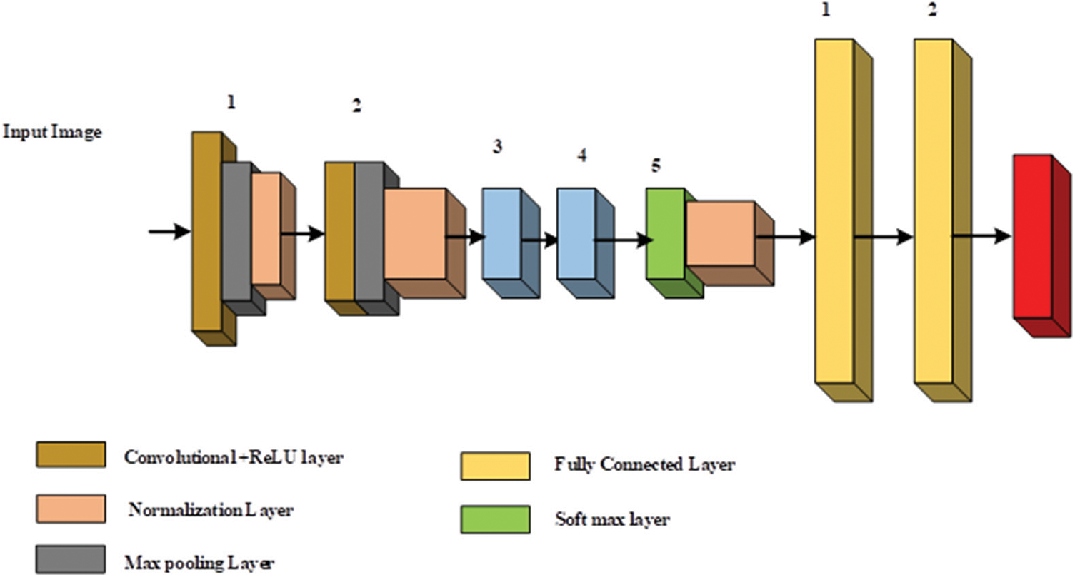
Figure 2: Structure of convolutional neural network

Each convolution layer (layer 1, layer 3 and layer 5), these layers can be convolved with the consideration of kernel size which formulated based on below formulation,

XN=∑k=0n−1⁡YkFN−k (5)

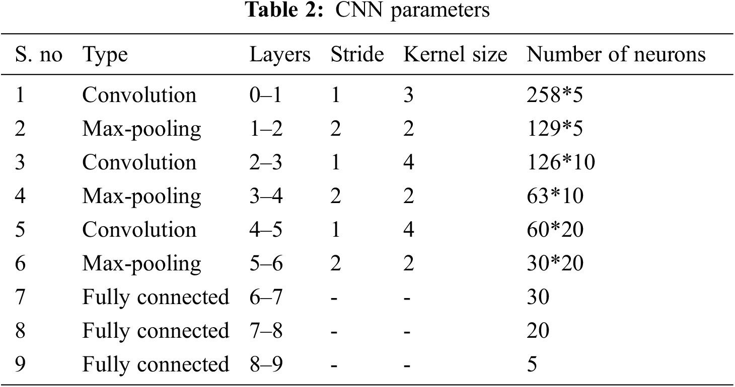
It is a convolution operation. Here, N can be described as number of elements, F can be described as filter and Y can be described as input image. After the convolution layer, the pooling operation is considered to attain feature maps. The requirement of max pooling can be decreasing the feature map size. The kernel size with the parameter is achieved with the help of Reinforcement Learning based optimization Algorithm (ROA) technique whereas the max pooling operation and convolution stride is fixed at 2 and 1. In the CNN, the activation function is taken as leaky rectifier linear unit in the layers of 1, 3, 5, 7 and 8. The fully connected layer contains of 5, 20 and 30 output neurons with the specified output layer. The Softmax function can be utilized to separate the segmented images with two classes such as segmented portion and remaining portion. The design parameters of the CNN are presented in Tab. 2.

The designed CNN is trained with the assistance of the backpropagation method based on the sample size, i.e., 10. The hyper parameter of the CNN also regularized with the assistance of ROA which are momentum, learning rate and regularization. This parameter is impeded data overfitting, manage the speed of training process and data convergence. The parameters are adjusted based on ROA technique to attain efficient outcomes. Additionally, the weights and biases are updated based on below formulation [20].

Here, c can be described as cost function, T can be described as updating step, M can be described momentum, N can be described as the total number of training set, X can be described as learning rate, λ can be described as regularization parameter, L can be described as layer number, b can be described as bias and w can be described as weight. Testing and training of the CNN is completed in 20 epochs. In the training and testing process, the 80% of image is utilized to training the network and remaining 20% is utilized to testing the network.

ΔwT(T+1)=−XλRwL−XN∂c∂wL+MΔwL(T) (6)

ΔwT(T+1)=−XN∂c∂bL+MΔbL(T) (7)

3.4 Honey Badger Algorithm

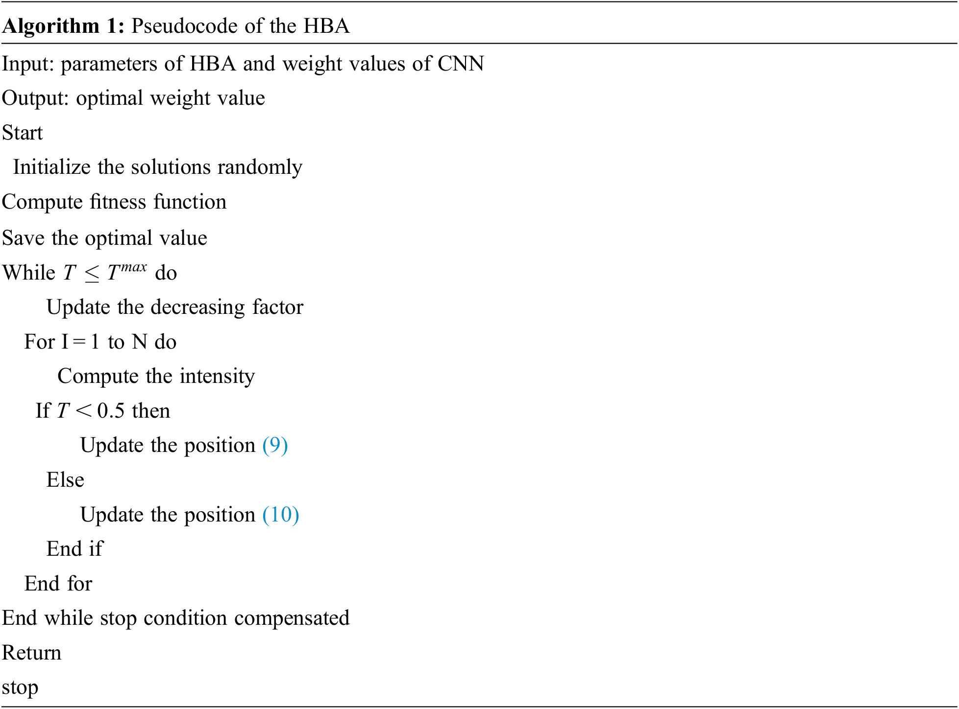
In the CNN, the HBA is utilized to select optimal weighting parameter The Honey Badger is a vertebrate originate in the rainforests of Africa and semi deserts. Indian subcontinent and southeast Asia and it named as during wildlife. This reed scope (60 towards 77 cm in body length in addition 7 towards 13 kg body weight) is a courageous foraging animal that hunts sixty unique creatures, including dangerous snakes. It is a brilliant creature that is ready to utilize gears, in addition its dear’s honey. It prefers solitude in self-drilled openings in addition encounters different pesters for mating. There are 12 honeys pester category. Honey badgers do not have a specific breeding season as the chicks are constantly being brought into the world. As a result of their heroic nature, it does not attack even large predators when it cannot escape. The HBA algorithm is developed based on the foraging characteristics of honey badger. Aimed at identifying food source, the honey badger moreover follows, digs in addition smells honeyguide bird. In the HBA, initial scenario is digging phase and additional is a honey stage. In the previous stage, the situation considered the sensing behaviour towards identify prey location while achieving the prey and it transfers around the prey to choose the required place of catching and digging the prey. Afterwards, the honey badger considers the honeyguide bird to straightly identify the location [21].

The HBA is working based on two mode of operation such as digging mode and honey mode. This portion provide the mathematical demotions of the HBA algorithm. Additionally, the HBA is connected with exploitation and exploration stage. Hence, this algorithm is named as global optimization algorithm. This algorithm is proceeding with three steps such as initialization, evaluation and updating functions. the population initialization is presented as follows,

Initialpopulation=[X11X12X13…X1dX21X22X23…X2d……………XN1XN2XN3…XN,D] (8)

The position of honey badger is formulated as follows,

XI=[XI1,XI2,…,XID] (9)

Step 1: Initialization stage:

Number of honey badgers are initialized based on their positions,

XI=LBI+R1×(UBI−LBI) (10)

where, R1 can be described as the random variable among 0 and 1, UBI can be described as the upper bounds of the search domain, LBI can be described as the lower bound of the search domain, XI can be described as the honey badger position related to a candidate solution.

Step 2: Fitness Evaluation

The fitness function is mathematically formulated as follows,

FF=MAX{PSNR} (11)

PSNR=10log10(MAXPMSE) (12)

MSE=1N∗M∑X=1N⁡∑Y=1M⁡[Iimage(A,B)−Id−image(A,B)]2 (13)

where, Id−image(A,B) is described as output labelled images and Iimage(A,B) is described as an input image. Based on the fitness function, the CNN parameters are selected which are utilized to enhance the optimal image annotation process.

Step 3: Described the intensity (I)

Intensity can be related with the concentration of the prey in addition distance among the honey badger. The intensity function of HBA is presented as follows,

II=R2×S4πDI2 (14)

S=(XI=XI+1)2 (15)

DI=XPrey−XI (16)

where, R2 can be described as the random variable among 0 to 1, DI  can be described as distance among prey and ith badger and S can be described as concentration strength or source strength.

Step 4: Density factor updating

In the HBA, the time varying randomization is controlled by density factor to empower smooth transition from exploitation to exploration. The decreasing the density factor, which reduce the iteration and reduce the randomization with respect to the time based on below equation,

α=C∗exp(−TTmax) (17)

where, Tmax can be described as the maximum number of iterations and C can be described as the constant parameter which taken as 2.

Step 5: Local optimum condition

In this step, local optima conditions are checked. This algorithm, the Flag F can be altered the search way intended aimed at achieving in height opportunities aimed at agent to scan the exploration interplanetary thoroughly.

Step 6: Agent position update.

The updating process is split into two sections such as digging phase and honey phase.

Digging phase:

During the digging phase, the cardioid motion can be computed as follows,

XNEW=XPrey+F∗β∗I∗XPrey+F∗R3∗α∗DI∗|cos(2πR4)∗[1−cos(2πR5)]| (18)

Here, F can be described as the flag which change the search direction, R3,R4,R5 can be described as the random variables among 0 and 1, DI can be described as the distance among the prey and ith honey badger, β can be described as the ability of the honey badger to achieve the food and XPrey can be described as the position of the prey.

The flag operation can be formulated as follows,

F={1ifR6≤0.5−1else (19)

where, R6 can be described as a haphazard number among 0 and 1. During the digging stage, time changing search influence factor, distance among the prey and badger and a honey badger can be depends on smell intensity. Additionally, throughout digging behaviour, a badger might get slightly trouble that permits it towards compute smooth optimal prey site.

The honey badger is following the honey guide bird towards to achieve the optimal results which formulated as follows,

Xnew=Xprey+F∗R1∗α∗Di (20)

where, R1 can be described as the random number among 0 to 1, Di can be described as the distance information, Xprey can be described as the honey badger prey location and Xnew can be described as the honey badger new position. The pseudocode of the projected technique is presented in algorithm 1.

Additionally, HBA can be related with the global optimization algorithm based on exploitation and exploration stages. To achieve efficient outcomes, the HBA [22] easy to understand and implement. Based on the HBA, the optimal weighting factors of the CNN is achieved.

4  Performance Evaluation

The performance of the projected technique is assessed in addition defensible in this portion. The proposed technique can be analyzed with performance metrices such as precision, recall, accuracy and F_Measure. To validate the projected technique of databases which is Corel 5k. This technique is implemented in MATLAB and performances are evaluated. It is contrasted with the conventional approaches such as CNN and HDNN.

4.1 Dataset Description

This is an explicitly accessible database that is commonly used for image description error. It is illustrated with 374 marks with 5000 images from 50 photo Compact Disk (CD). Each CD will memorize 100 images to a similar point, illustrated with 1–5 tracking words for each image. Due to the misconception about the circulation of notes on images, most past works think about using two-dimensional ideas (i.e., subgroups of images) that are repeated each time. Nevertheless, we evaluate the proposed calculation in both the subset and the complete set of data, demonstrating its reliability and resistance to the problem of intermediate mark smuggling. The Corel-5 K is currently divided into rail and test subgroups, which include 4500 and 500 images. The sample input image of Corel 5k dataset is presented in the Fig. 3. With the consideration of databases, the performance of the projected approach is achieved by using different measures such as accuracy, precision, recall, sensitivity, F_Measure and kappa.

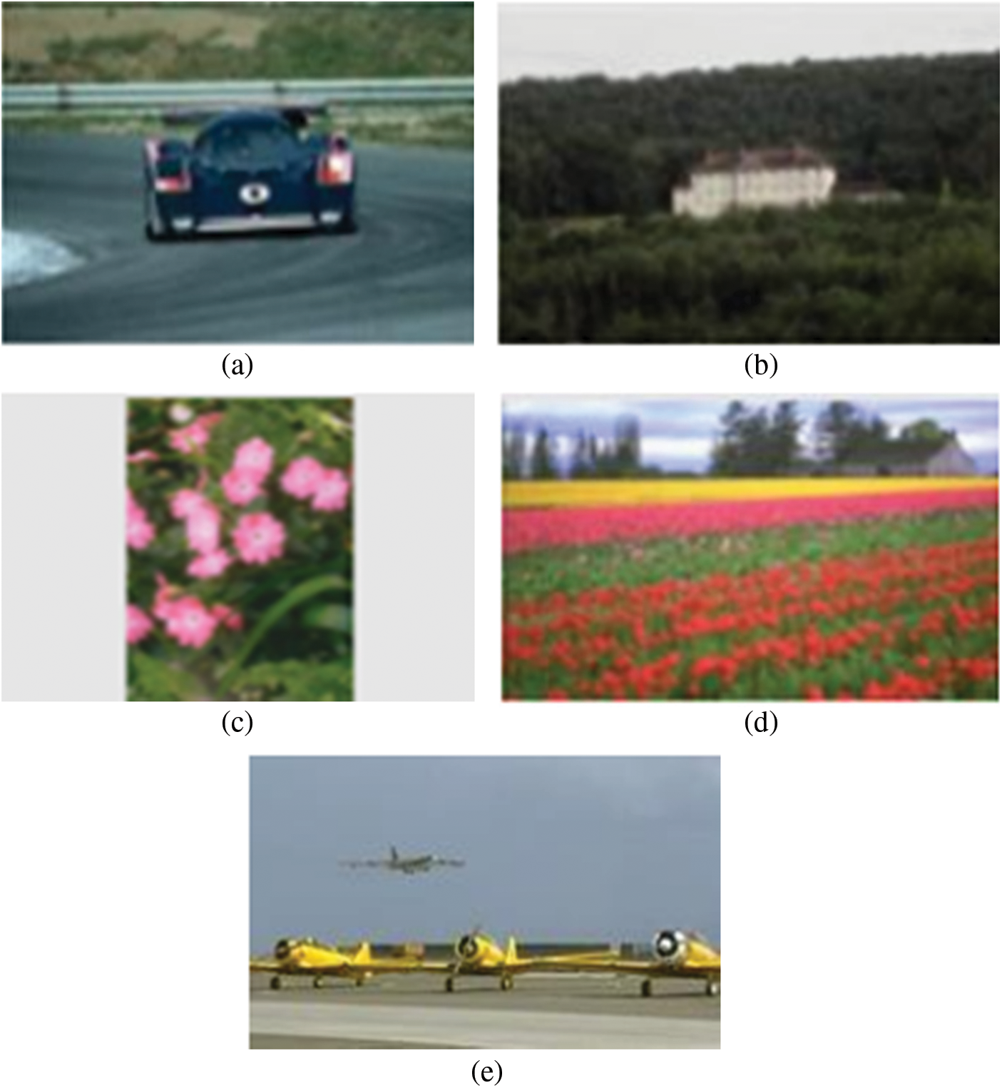
Figure 3: Sample dataset (a) Car, tracks, grass (b) sky, tree, castle, (c) flowers, petals, leaf (d) flowers, tree, sky and (e) sky, plane, runway

The comparison analysis is presented in Tab. 3. The accuracy is a performance metric for evaluating the projected approach which is presented in Fig. 4. The projected approach attained the 96.3% of accuracy in the epoch 60. Additionally, the HDNN and CNN attained 94.85% and 93.2% accuracy in the epoch 60. Based on the analysis, the projected approach attained efficient accuracy. The precision is a performance metric for evaluating the projected approach which is presented in Fig. 5. The projected approach attained 96.5% of precision in the epoch 60. Additionally, the HDNN and CNN attained 94.82% and 93.8% precision in the epoch 60. Based on the analysis, the projected approach attained efficient results in terms of precision. The recall is a performance metric for evaluating the projected approach which is presented in Fig. 6. The projected approach attained 93.5% of recall in the epoch 60. Additionally, the HDNN and CNN attained 93.81% and 92.18% recall in the epoch 60. The specificity is a performance metric for evaluating the projected approach which is presented in Fig. 7. The projected approach attained 96.12% of specificity in the epoch 60. Additionally, the HDNN and CNN attained 93.12% and 94.52% specificity in the epoch 60. Based on the analysis, the projected approach attained efficient outcomes in terms of specificity. The F_Measure is a performance metric for evaluating the projected approach which is presented in Fig. 8. The projected approach attained 95.45% of F_Measure in the epoch 60. Additionally, the HDNN and CNN attained 94.12% and 93.02% F_Measure in the epoch 60. The kappa is a performance metric for evaluating the projected approach which is presented in Fig. 9. The projected approach attained 95.58% of kappa in the epoch 60. Additionally, the HDNN and CNN attained 94.98% and 93.58% kappa in the epoch 60.

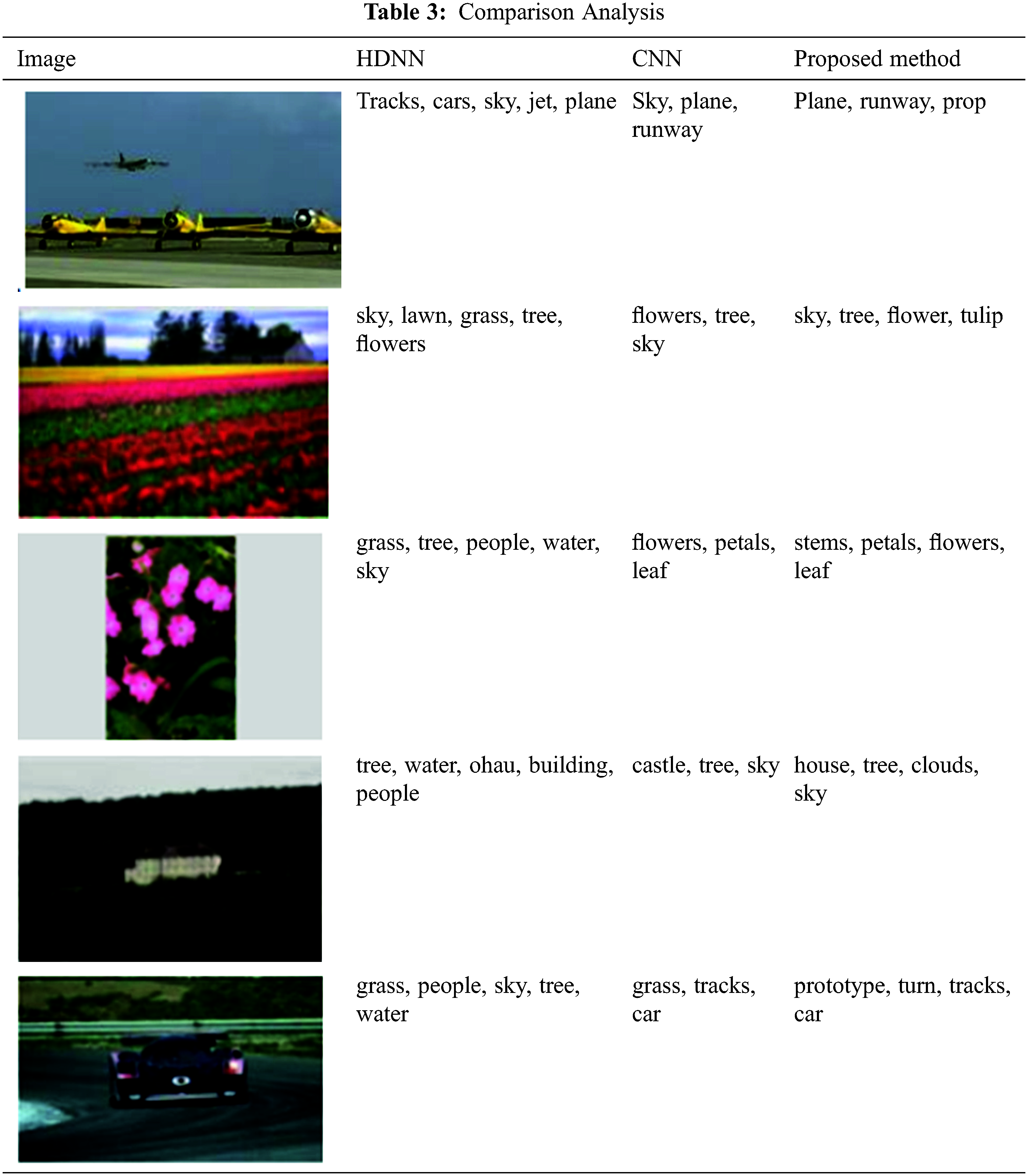
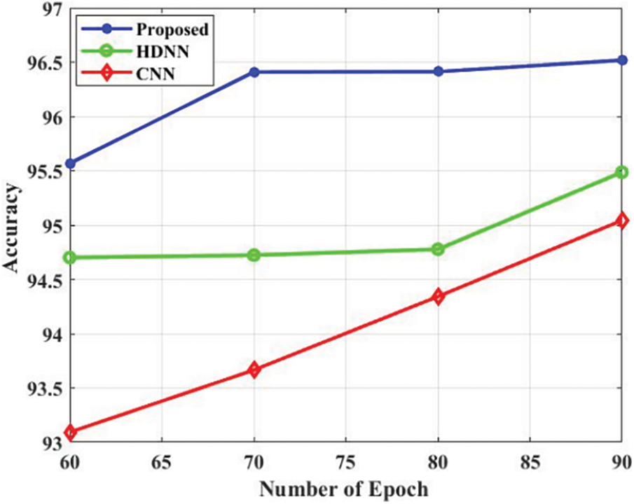
Figure 4: Accuracy

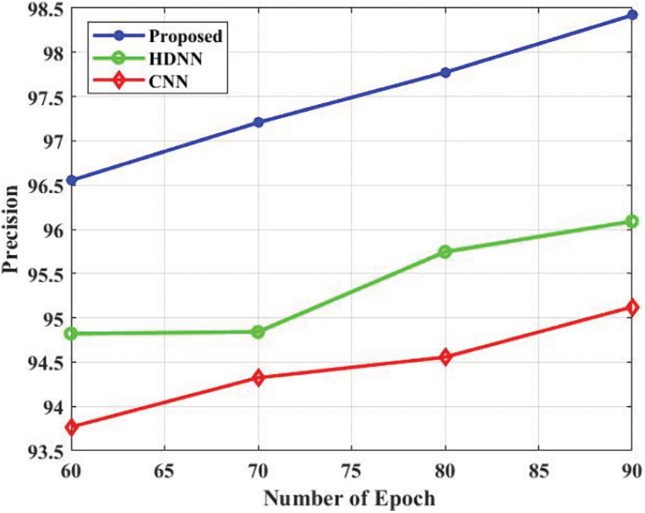
Figure 5: Precision

Figure 6: Recall

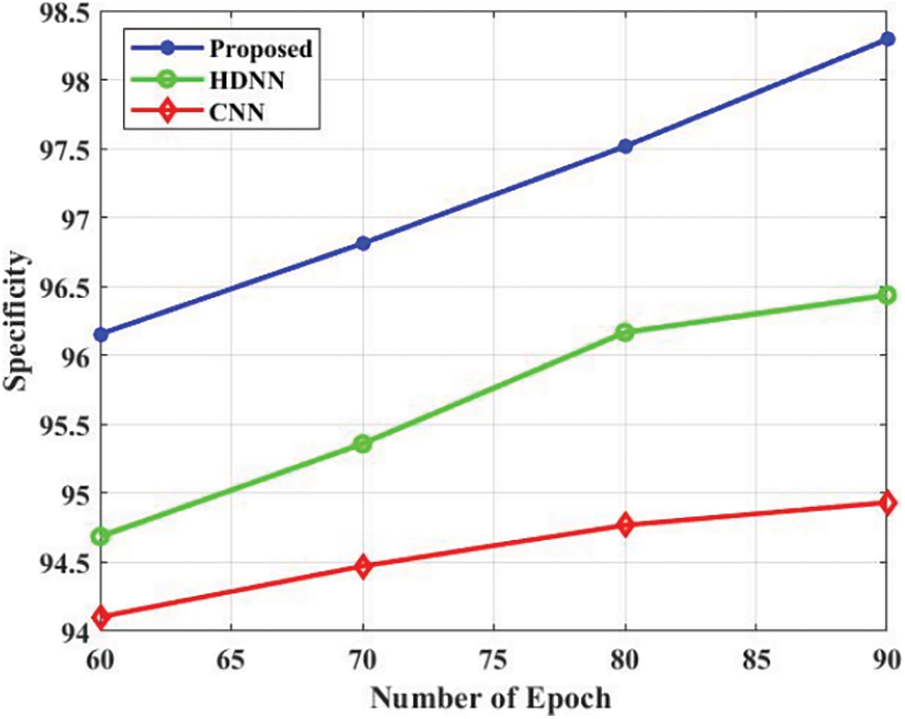
Figure 7: Specificity

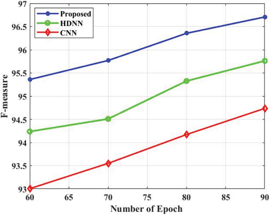
Figure 8: F_Measure

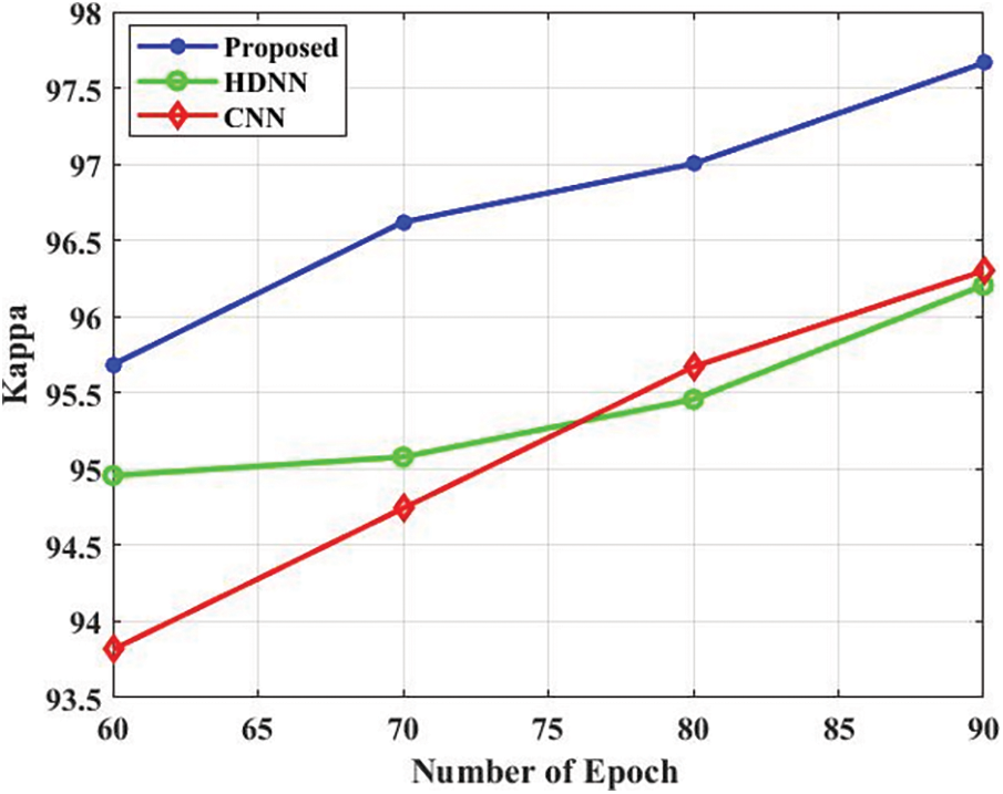
Figure 9: Kappa

5  Conclusion

In this paper, ACDLM has been developed for automatic image annotation. Initially, the database has been collected from the open-source system which consists of some labelled images (for the training phase) and some unlabeled images {Corel 5 K, MSRC v2}. After that, the image has been sent to the pre-processing step such as color space quantization and texture color class map. The pre-processed image has been sent to the segmentation approach for efficient labelling technique JSEG. The final step is an automatic annotation using ACDLM which is a combination of CNN and HBA. Based on the proposed classifier, the unlabeled images are labelled. The proposed methodology has been implemented using MATLAB and a performance is evaluated using performance metrics such as accuracy, precision, recall and F1_Measure. With the assistance of the proposed methodology, the unlabeled images are labelled. The projected technique attained an accuracy of 96.3%. In the future, other unlabeled images will be considered to enhance the performance of the approach.

Funding Statement: The authors received no specific funding for this study.

Conflicts of Interest: The authors declare that they have no conflicts of interest to report regarding the present study

References

1. Q. Cheng, Q. Zhang, P. Fu, C. Tu and S. Li, “A survey and analysis on automatic image annotation,” Pattern Recognition, vol. 79, pp. 242–259, 2018. [Google Scholar]
2. Y. Ma, Y. Liu, Q. Xie and L. Li, “CNN-Feature based automatic image annotation method,” Multimedia Tools and Applications, vol. 78, no. 3, pp. 3767–3780, 2019. [Google Scholar]
3. D. Rubin, M. Ugur Akdogan, C. Altindag and E. Alkim, “ePAD: An image annotation and analysis platform for quantitative imaging,” Tomography, vol. 5, no. 1, pp. 170–183, 2019. [Google Scholar]
4. R. Huang, F. Zheng and W. Huang, “Multilabel remote sensing image annotation with multiscale attention and label correlation,” IEEE Journal of Selected Topics in Applied Earth Observations and Remote Sensing, vol. 14, pp. 6951–6961, 2021, https://doi.org/10.1109/JSTARS.2021.3091134. [Google Scholar]
5. Y. Ma, Q. Xie, Y. Liu and S. Xiong, “A weighted KNN-based automatic image annotation method,” Neural Computing and Applications, vol. 32, no. 11, pp. 6559–6570, 2020. [Google Scholar]
6. E. Heim, T. Ross, A. Seitel, K. März, B. Stieltjes et al., “Large-scale medical image annotation with crowd-powered algorithms,” Journal of Medical Imaging, vol. 5, no. 3, pp. 829–832, 2018, https://doi.org/10.1117/1.JMI.5.3.034002. [Google Scholar]
7. J. Cao, A. Zhao and Z. Zhang, “Automatic image annotation method based on a convolutional neural network with threshold optimization,” Plos one, vol. 15, no. 9, pp. 1–21, 2020, https://doi.org/10.1371/journal.pone.0238956. [Google Scholar]
8. M. Moradi, A. Madani, Y. Gur, Y. Guo and T. Syeda-Mahmood, “Bimodal network architectures for automatic generation of image annotation from text,” in Int. Conf. on Medical Image Computing and Computer-Assisted Intervention, pp. 449–456, 2018, Granada, Spain, https://doi.org/10.1007/978-3-030-00928-1_51. [Google Scholar]
9. Z. Mehmood, T. Mahmood and M. A. Javid, “Content-based image retrieval and semantic automatic image annotation based on the weighted average of triangular histograms using support vector machine,” Applied Intelligence, vol. 48, no. 1, pp. 166–181, 2018, http://dx.doi.org/10.1007/s10489-017-0957-5. [Google Scholar]
10. H. Song, P. Wang, J. Yun, W. Li, B. Xue et al., “A weighted topic model learned from local semantic space for automatic image annotation,” IEEE Access, vol. 8, pp. 76411–76422, 2020. [Google Scholar]
11. M. M. Adnan, M. S. Rahim, A. R. Khan, T. Saba, S. M. Fati et al., “An improved automatic image annotation approach using convolutional neural network-slantlet transform,” IEEE Access, vol. 10, pp. 7520–7532, 2022. [Google Scholar]
12. Y. Niu, Z. Lu, J. Wen, T. Xiang and S. Chang, “Multi-modal multi-scale deep learning for large-scale image annotation,” IEEE Transactions on Image Processing, vol. 28, no. 4, pp. 1720–1731, 2018. [Google Scholar]
13. K. A. Philbrick, A. D. Weston, Z. Akkus, T. L. Kline, P. Korfiatis et al., “RIL-Contour: A medical imaging dataset annotation tool for and with deep learning,” Journal of Digital Imaging, vol. 32, no. 4, pp. 571–581, 2019. [Google Scholar]
14. P. Zhu, Y. Tan, L. Zhang, Y. Wang, J. Mei et al., “Deep learning for multilabel remote sensing image annotation with dual-level semantic concepts,” IEEE Transactions on Geoscience and Remote Sensing, vol. 58, no. 6, pp. 4067–4060, 2020. [Google Scholar]
15. W. Sun, X. Chen, X. Zhang, G. Dai, P. Chang et al., “A Multi-feature learning model with enhanced local attention for vehicle re-idenpngication,” Computers, Materials & Continua, vol. 69, no. 3, pp. 3549–3561, 2021. [Google Scholar]
16. S. Karthic and S. Manoj Kumar, “Wireless intrusion detection based on optimized lstm with stacked auto encoder network,” Intelligent Automation & Soft Computing, vol. 34, no. 1, pp. 439–453, 2022. [Google Scholar]
17. M. Frackiewicz and H. Palus, “KM and KHM clustering techniques for colour image quantisation,” Computational Vision and Medical Image Processing, pp. 161–1741, 2011, Switzerland: Springer International Publishing, https://doi.org/10.1007/978-94-007-0011-6_9. [Google Scholar]
18. R. Bensaci, B. Khaldi, O. Aiadi and A. Benchabana, “Deep convolutional neural network with KNN regression for automatic image annotation,” Applied Sciences, vol. 11, no. 21, pp. 1–20, 2021, https://doi.org/10.3390/app112110176. [Google Scholar]
19. U. R. Acharya, S. L. Oh, Y. Hagiwara, J. H. Tan, M. Adam et al., “A deep convolutional neural network model to classify heartbeats,” Computers in Biology and Medicine, vol. 89, no. 1, pp. 389–396, 2017. [Google Scholar]
20. R. K. Kaliyar, A. Goswami, P. Narang and S. Sinha, “FNDNet–a deep convolutional neural network for fake news detection,” Cognitive Systems Research, vol. 61, pp. 32–44, 2020. [Google Scholar]
21. F. A. Hashim, E. H. Houssein, K. Hussain, M. S. Mabrouk and W. Al-Atabany, “Honey badger algorithm: New metaheuristic algorithm for solving optimization problems,” Mathematics and Computers in Simulation, vol. 192, pp. 84–110, 2022. [Google Scholar]
22. E. Han and N. Ghadimi, “Model idenpngication of proton-exchange membrane fuel cells based on a hybrid convolutional neural network and extreme learning machine optimized by improved honey badger algorithm,” Sustainable Energy Technologies and Assessments, vol. 52, 2022, https://doi.org/10.1016/j.seta.2022.102005. [Google Scholar]
Cite This Article
Copyright © 2023 The Author(s). Published by Tech Science Press.
This work is licensed under a Creative Commons Attribution 4.0 International License , which permits unrestricted use, distribution, and reproduction in any medium, provided the original work is properly cited.
Downloads
Citation Tools