
 Submit a Paper
 Propose a Special lssue
 Open Access
ARTICLE
Estimation of Higher Heating Value for MSW Using DSVM and BSOA
Sathyabama Institute of Science and Technology, Chennai, 600119, India
* Corresponding Author: Jithina Jose. Email:
Intelligent Automation & Soft Computing 2023, 36(1), 573-588. https://doi.org/10.32604/iasc.2023.030479
Received 27 March 2022; Accepted 28 June 2022; Issue published 29 September 2022
 View Full Text
 Download PDF
Abstract
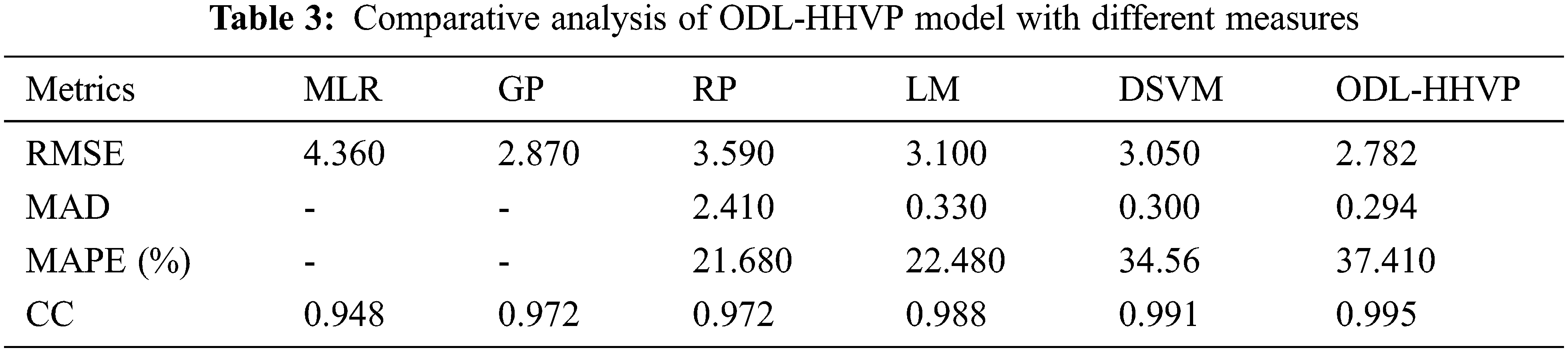
In recent decades, the generation of Municipal Solid Waste (MSW) is steadily increasing due to urbanization and technological advancement. The collection and disposal of municipal solid waste cause considerable environmental degradation, making MSW management a global priority. Waste-to-energy (WTE) using thermochemical process has been identified as the key solution in this area. After evaluating many automated Higher Heating Value (HHV) prediction approaches, an Optimal Deep Learning-based HHV Prediction (ODL-HHVP) model for MSW management has been developed. The objective of the ODL-HHVP model is to forecast the HHV of municipal solid waste, based on its oxygen, water, hydrogen, carbon, nitrogen, sulphur and ash constituents. In addition, the ODL-HHVP model contains a Deep Support Vector Machine (DSVM) regression component that can accurately predict the HHV. In addition, the Beetle Swarm Optimization (BSO) method is utilised as a hyperparameter optimizer in conjunction with the DSVM model, resulting in the highest HHV prediction accuracy. A comprehensive simulation study is conducted to validate the performance of the ODL-HHVP method. The Multiple Linear Regression (MLR), Genetic Programming (GP), Resilient backpropagation (RP), Levenberg Marquardt (LM) and DSVM approaches have attained an ineffective result with RMSEs of 4.360, 2.870, 3.590, 3.100 and 3.050, respectively. The experimental findings demonstrate that the ODL-HHVP technique outperforms existing state-of-art technologies in a variety of respects.Keywords
Municipal Solid Waste (MSW) rates are increasing due to the consequence of fast technological development and urbanization. The disposal and collection of municipal solid waste worsen environmental problems, making MSW management a critical global concern [1]. Waste To Energy (WTE) using thermochemical process appears to yield potential answer in this field. Given their variety and diversity, it is vital to comprehend the components. In reality, there are three independent methods for evaluating composition as follows: ultimate, physical and proximate analyses [2]. Physical analysis of municipal solid waste includes biodegradable components derived from biomass, wood, food, paper, cardboard and cotton and non-biodegradable components derived from fossil fuels, rubber and plastics. The final analysis considers the amount of hydrogen (H), carbon (C), sulphur (S), oxygen (O) and nitrogen (N) (N). Estimating the quantities of volatile matter, moisture, ash and fixed carbon using proximate analysis [3,4]. Similarly, thermal parameters such as heating values, notably the Higher Heating Value (HHV) [5,6], play a significant role in the design of WTE plants. Investigative determinations incur high expenditures [7]. Following that, researchers centred their efforts on developing empirical models for determining the calorific values of an important component. Typically, the HHV model is utilised to determine the fundamental composition of prospective resources such as biomass and coal.
MSW consists of a wide variety of chemicals from which energy may be recovered by various conversion techniques, including biological, thermochemical, anaerobic digestion, pyrolysis and combustion [8–10]. However, designing unique methods for extracting fuels from MSW requires a grasp of the MSW’s important properties, notably its High Heating Value (HHV) and elemental composition, which provide professionals’ insight into the MSW’s value for fuel generation [11–13]. The heating value is used to determine the amount of energy recovered from waste during conversion [14,15]. Even if the heating values are measured experimentally using a bomb calorimeter, the present global economic trend demands assessing the heating value of MSW in order to reduce the cost of energy generation. Routine information, such as the concentration of sulphur, moisture, oxygen, hydrogen, carbon and nitrogen in MSW ash, enables rapid MSW usage decision. This will also give personal knowledge regarding the gaseous emissions and potential for global warming caused by municipal solid waste. Numerous models have been presented [16] based on investigative data from waste moisture content, gravimetric composition and proximal and final studies. However, the bulk of these models fail to account for the nonlinear relationships of MSW. Consequently, a knowledge vacuum exists regarding the HHV prediction of MSW [17]. When a change in one feature does not result in a change in another, MSW has a nonlinear dependence. For instance, a change in the carbon/moisture content of municipal solid waste (MSW) is not proportional to a change in the hydrogen, oxygen, sulphur, or nitrogen contents.
Through final analysis, Boumanchar et al. [18] constructed an empirical model for predicting MSW-HHV. Formalization of genetic programming and multiple regression analysis were used as approaches and produced a superior outcome. In terms of CC and RMSE, genetic programming delivers greater accuracy than earlier research. Sankaralingam et al. [19] proposed a municipality-based technique for calculating trash Lower Heating Value (LHV) that overcomes the shortcomings of generic methodologies by considering the features and idiosyncrasies of locally produced rubbish. The Adaptive Network-based Fuzzy Inference System (ANFIS) and Artificial Neural Networks (ANN) algorithms are provided with input variables with the percentage composition of waste streams such as plastics, paper, glass, organic and textile and output variables of LHV.
During inference, Melinte et al. [20] concentrated on enhancing the generalization, detection speed and accuracy of a pretrained Convolutional Neural Network (CNN) Object Detector. The pipeline consists of data enrichment, box predictor modules and CNN feature extraction for classification and localization at varying feature map sizes. The training models are constructed with deduction in mind. Alotaibi et al. [21] created an MPANN for forecasting HHV in municipal solid waste. The anticipated HHV is related to the investigational data using two separate trained functions, Resilience and Levenberg Marquardt back propagation.
Using an artificial neural network and multivariate linear regression, Prakash et al. [22] predicted LHV. This data-driven model describes the LHV and wet physical components of MSW by using 151 widely dispersed datasets uncovered during a systematic investigation. Ighalo et al. [23] described a novel method for predicting the HHV of biomass in machine learning using a Linear Regression Algorithm (LRA) and a Stochastic Gradient Descent (SGD). The main models integrate 78 lines of proximal and final analytical data. The precision of LRA model is stressed.
Li et al. [24] developed an ANN forecasting model for syngas HHV utilising process parameters (catalyst type, sludge type, pyrolysis temperature, moisture content and catalyst amount). Initially, a three-phase network consisting of one output neuron, eight input neurons and fifteen hidden neurons is determined by boosting various sets of parameters. Using an ANN model, the HHV of syngas is therefore appropriately predicted. Using artificial neural networks, Pattanayak et al. [25] estimated the HHV of bamboo biomass. Using inputs from ultimate, proximal and integrated analysis, the three ANN approaches are introduced. Statistical and graphical comparisons of inquiry data are used to assess the correctness of this model’s predictions. It has been established that ANN methods can predict HHV in biomass with greater precision.
Cubillos [26] examined the benefits of complicated DL models over more conventional prediction methods. Using a long-term database, a multi-site LSTM-NN is employed to predict the residential garbage generation rates. These models are based on historical information on home waste in Herning, Denmark. Prakash et al. [27] examined the prediction of HHV valuations using Multi-Layer Perceptron Artificial Neural Network (MLP-ANN) and Least Squares Support Vector Machine computations (LSSVM).
Recent research identifies municipal solid waste as a significant renewable energy source. The heating value of municipal solid waste is a crucial variable for MSW-based energy solutions. Frequently, heating values are obtained experimentally with a bomb calorimeter. In contrast, the calorimetric method requires time-consuming manual laboratory work. For saving time and reducing costs associated with the operation and construction of MSW-based engineering systems, it is necessary to develop models for reliable estimate of heating values in such situations.
This paper examines the development of an Optimal Deep Learning-based HHV Prediction (ODL-HHVP) model for MSW management, with the objective of predicting the HHV of MSW based on the concentrations of oxygen, water, hydrogen, carbon, nitrogen, sulphur and ash. In addition, the HHV prediction process may be viewed as a regression issue that can be solved using a Deep Support Vector Machine (DSVM). Beetle Swarm Optimization (BSO) is utilised to fine-tune the DSVM model’s parameters, resulting in a significant increase in prediction output. Originality is exemplified by BSO method for fine-tuning the DSVM model for HHV prediction. Extensive experimental validation is conducted and the outcomes are analysed on various levels.
2.1 Characterization of Biomass
The waste biomass gathered in Chennai, Tamil Nadu, India, in a municipal solid waste disposal yard is dried and processed into a fine powder. The carbon, hydrogen, nitrogen, sulphur, water and ash contents of biomass are determined and used as input parameters. The moisture content and ash content of gathered biomasses are determined using ASTM standards. The elemental composition of biomass (carbon, hydrogen, nitrogen, sulphur and oxygen) is determined using an elemental analyzer (Perkin-Elmer 2400 series CHNS analyzer).
2.2 High Temperature Prediction
The amount of energy produced by oxidation of biomass is known as its high heating value (HHV). The High Heating Value is a crucial factor in defining the characteristics of biomass (HHV). Frequently, a Bomb calorimeter is used to estimate the HHV of biomass. For biomass fuels, the Proximate and Ultimate composition-based formulae are utilised. The Proximate Analysis determines the biomass’s fixed carbon, volatile carbon and ash content. In the Final Analysis, the Critical Components are determined (C, H, O, S and N). MSW is a composite substance composed of several different substances. The enthalpy of combustion varies significantly according to the kinds of waste. Several HHV models for biomass have been developed based on the elemental makeup of the biomass. Below are some HHV forecasting formulae.
Kathiravale et al. used the following equation for calculating HHV in KJ/Kg
Meraz et al. used following formula for calculating HHV in MJ/Kg
Shi et al. presented another equation
2.3 The Proposed ODL-HHVP Technique
The objective of this study is to develop a novel ODL-HHVP method for predicting HHV based on the concentrations of oxygen, water, hydrogen, carbon, nitrogen, sulphur and ash. The proposed ODL-HHVP technique comprises of two phases: regression using DSVMs and parameter tuning with BSOs. Fig. 1 displays the procedure of the ODL-HHVP model. The subsequent sections explain in detail how these modules function.
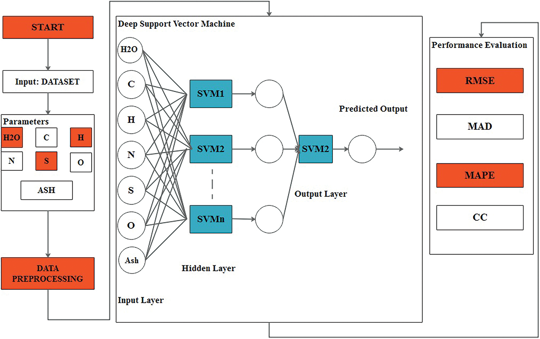
Figure 1: Overall process of ODL-HHVP (Optimal deep learning based HHV Prediction) model
2.3.1 Design of DSVM Based Predictive Model
A collection of input parameters is originally provided to the DSVM model in order to estimate the HHV value. Paper, plastic, fabric, food, wood, yard waste, glass, metals and ash are examples of waste. Carbon (C), hydrogen (H), nitrogen (N), oxygen (O), sulphur (S), ash and water content are used to generate the HHV output parameters. Consider the next regression sample:
That iteratively computes all elements in
It adjusts the SVM coefficient of each SVM via min-max formula of the binary objectives W of the primary SVM [28].
They have proposed a gradient ascent model for training the SVM. The methods adapt the SVMs coefficient α(*) (stands for each
They use RBF kernel in a 2 layered DSVM. The result with another kernel is worsening for the primary SVM.
The model constructs novel datasets for all feature layers of SVM
whereas μ represents the learning rate and
The feature extract SVM is launched pseudo-randomly and the training of the primary and featured layer SVMs is iterated across a number of epochs. Subtracting the average error from the total error yields the bias value. Determine the best learning rate to improve classification accuracy.
2.3.2 Design of BSO Based Parameter Tuning Process
The BSO approach is used for DSVM parameter tuning. BSA is a clever optimization approach that replicates the behaviour of beetles while foraging. After foraging, a beetle will use both of its antennae to determine the potency of a food’s aroma. If the scent intensity obtained by the left antennae is greater, it will fly towards the left; otherwise, it will fly towards the right. The technique outlined below is utilised to model BAS algorithm.
Dim, on the other hand, represents the spatial dimension. The right and left antennae of the beetles’ spatial coordinates are defined by,
t is the step factor, sign specifies a sign function and eta denotes the variable step factor, which is typically 0.95.
The BSO algorithm is utilised to optimise the performance of the BSA. BSO is an optimization strategy that combines the beetle foraging process with the Particle Swarm Optimization (PSO) method. Numerous papers have been devoted to the two antennae used by beetles to discover neighbouring areas. When one antenna senses very intense food odours from one direction, the beetle will travel toward the opposite antennae. The foraging behaviour of beetles was utilised to construct a meta-heuristic optimum model with a basic biological basis. It is described with the location of beetle from S-dimensional space at t as
Here,
The BSO concept is insufficient for high-definition operations and the primary antenna site is the most susceptible. The method by which a beetle increases its speed may be quantified by comparing the tendency of BSO to pursue global extreme rates to each insect’s pursuit of individual extremes. This could not be estimated by increasing the speed of the matching antennae, in contrast to the enhancement of each insect’s location. In order to develop a more intelligent computer model, it employs a method of loosening.
Figure 2: Flowchart of BSO (Beetle Swarm Optimization)
Therefore, the updates of position and speed of BSO framework are provided in the following equations.
where
The BSO algorithm selects an individual based on their fitness levels, then calculates the ideal solution based on the outcome of each individual. MSE is used as a fitness function in this study and the objective is to reduce MSE. It displays an error range between the predicted and actual DSVM values. This is demonstrated by the following example:
where
The suggested model’s performance is validated using the given dataset [30]. Tab. 1 and Fig. 3 illustrate the sample distribution of the dataset. The values provide the maximum, minimum, mean and standard deviation for each component of the dataset.
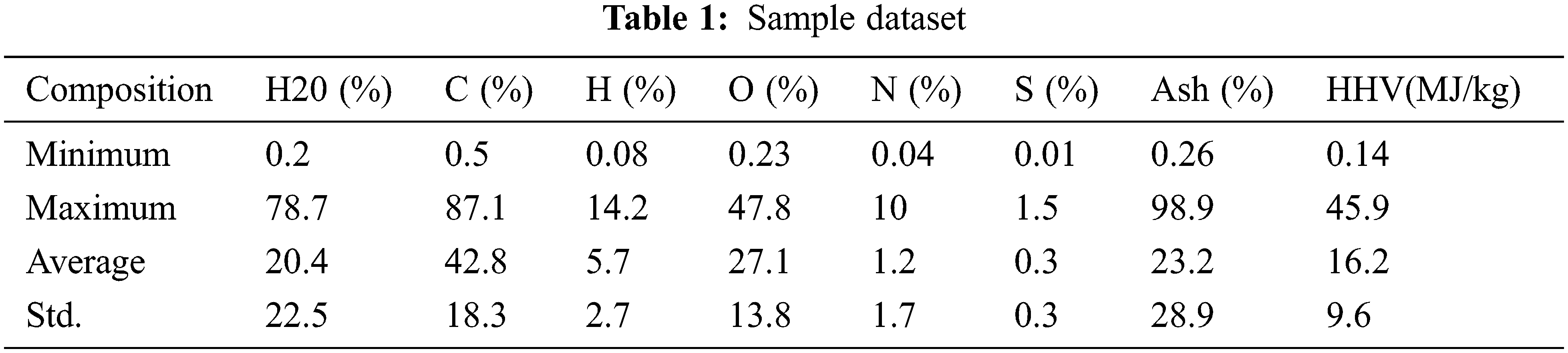
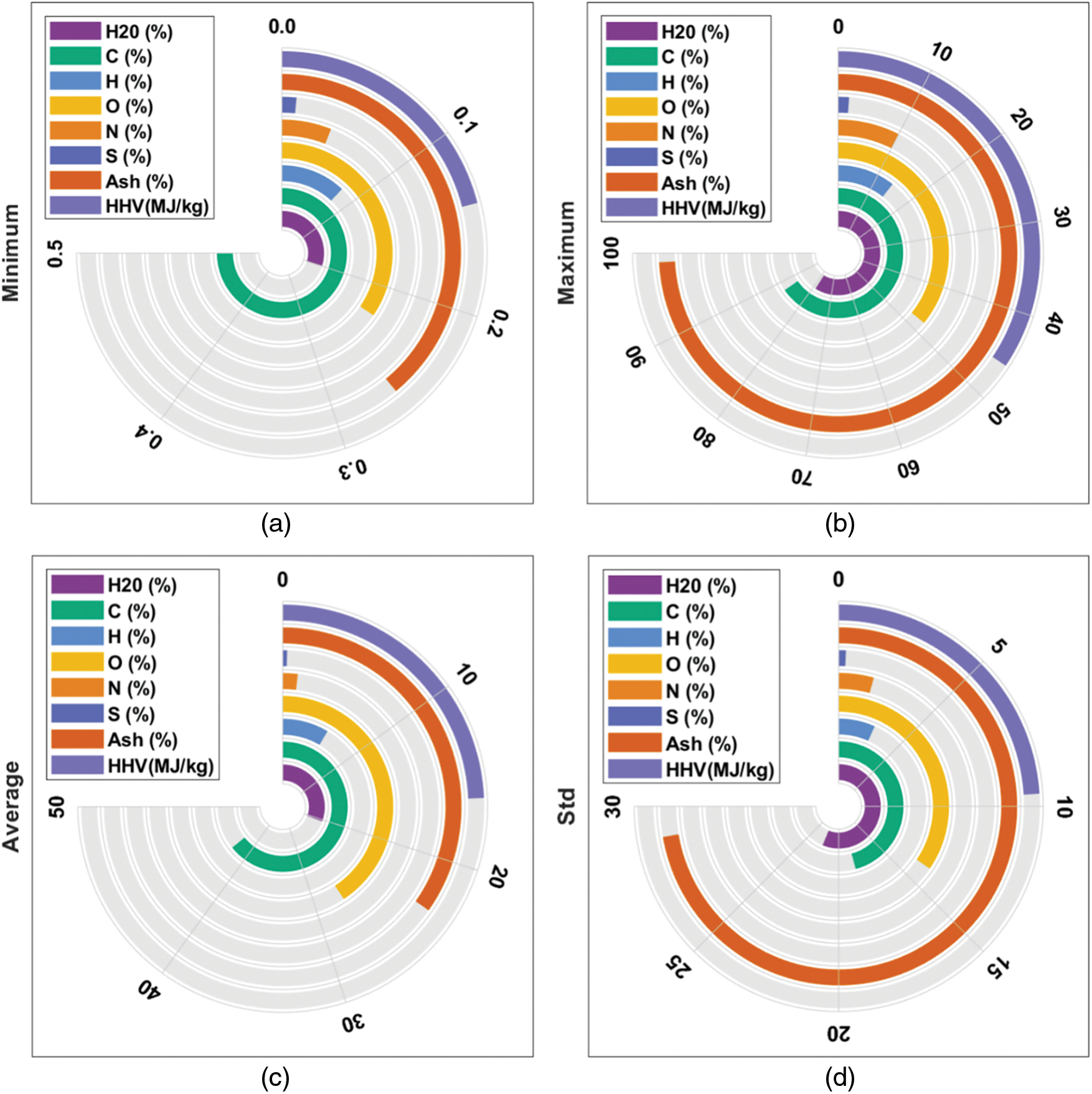
Figure 3: Sample dataset
The HHV outcomes predicted by the DSVM and ODL-HHVP models are evaluated in Tab. 2 and Figs. 4 and 5. On employing unique data indexes, the ODL-HHVP technique yields a small discrepancy between observed and predicted values. Using five data indices, the DSVM and ODL-HHVP techniques have predicted HHV concentrations of 21.81 and 20.37 MJ/kg, respectively, but the actual concentration is 19.54 MJ/kg. The DSVM and ODL-HHVP approaches projected an HHV of 2.33 and 2.36 MJ/kg, respectively, based on 10 data indices, but the actual HHV is 2.40 MJ/kg.
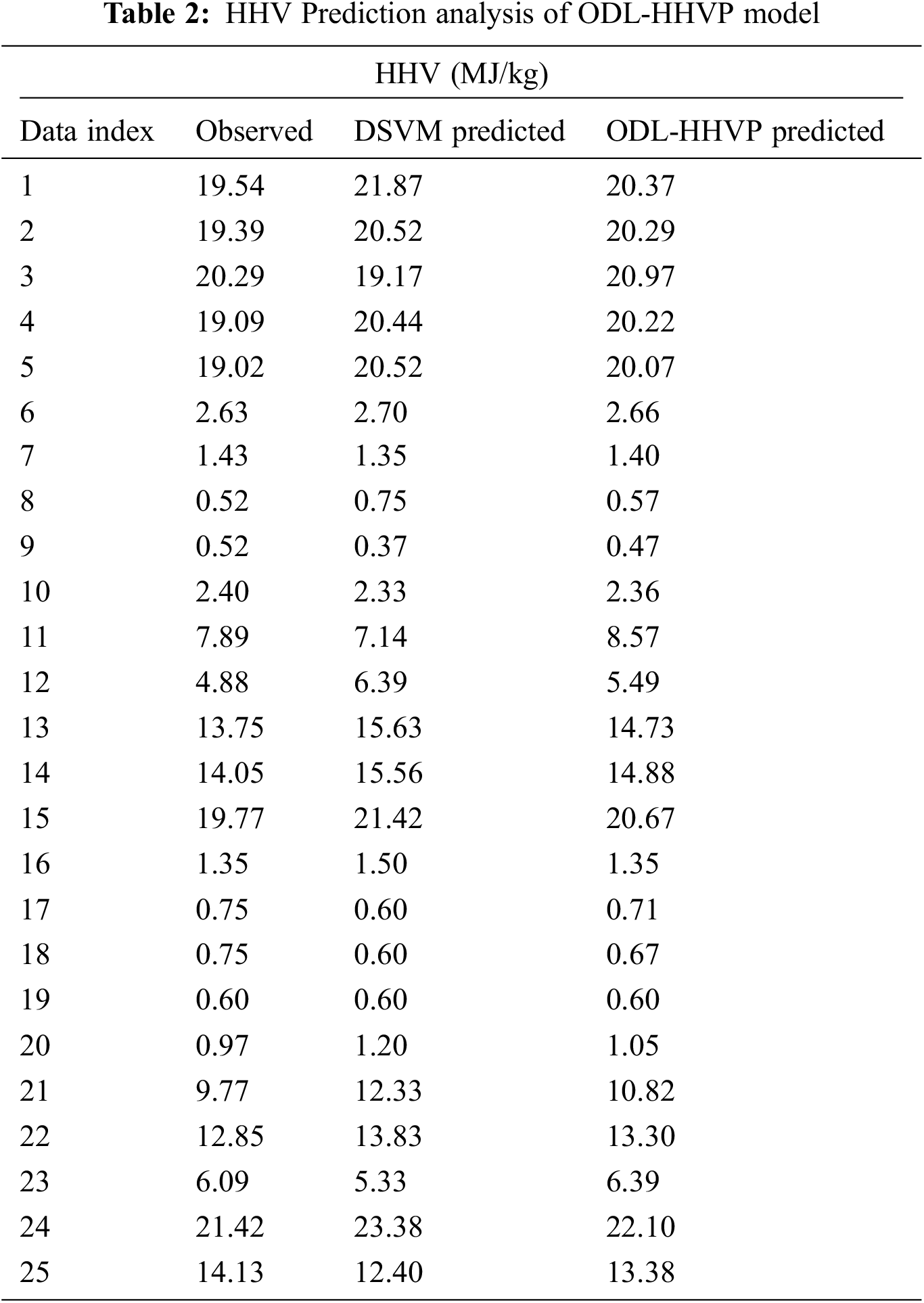
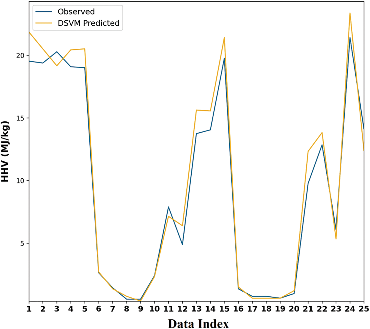
Figure 4: HHV prediction result analysis of DSVM (Deep Support Vector Machine) Model-I
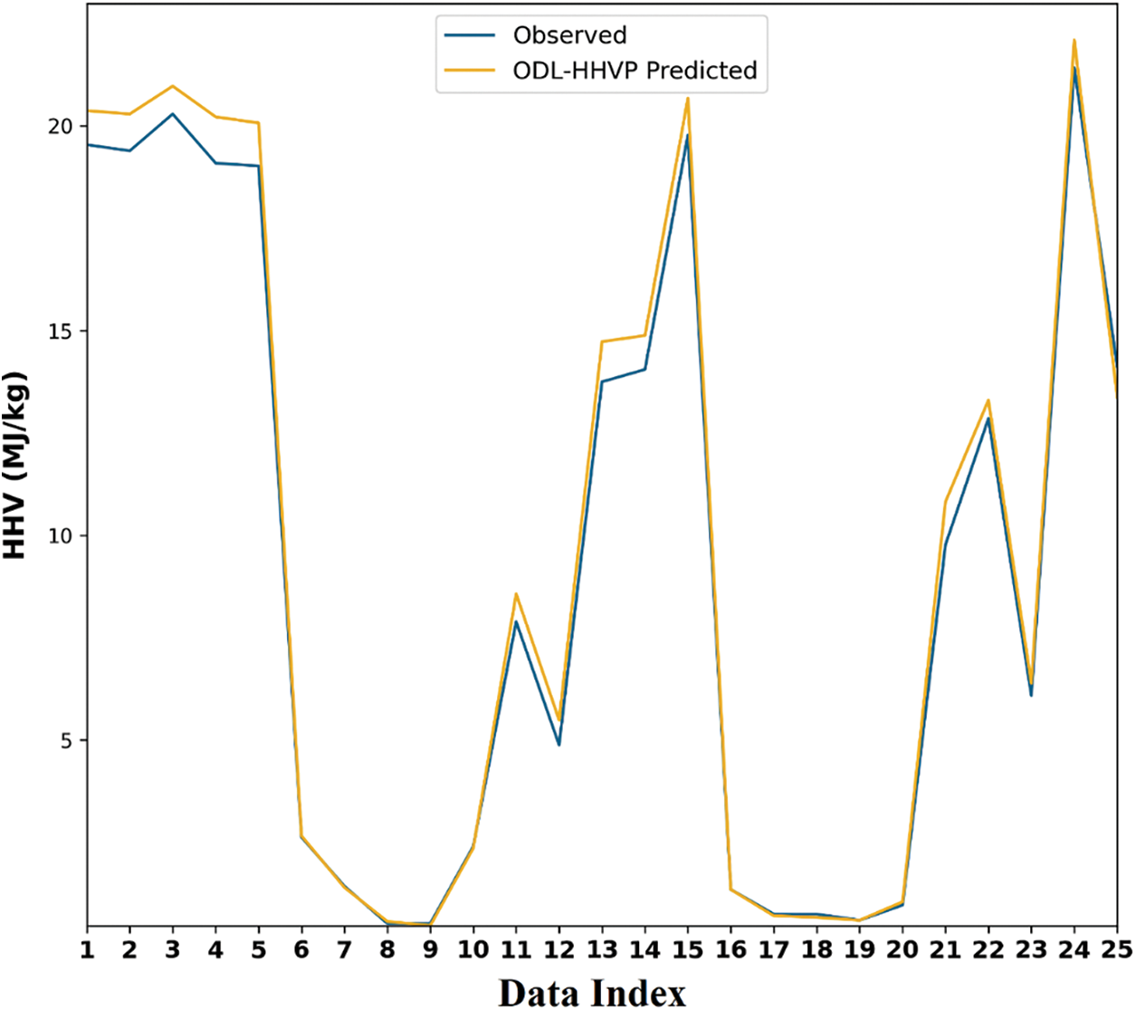
Figure 5: HHV prediction result analysis of DSVM model-II
Using 12 data indices, the DSVM and ODL-HHVP methods predicted HHV concentrations of 6.39 and 5.49 MJ/kg, respectively, but the actual HHV concentration is 4.88 MJ/kg. In addition, the DSVM and ODL-HHVP methods predicted HHV concentrations of 21.42 and 20.67 MJ/kg, respectively, but the actual concentration is 19.77 MJ/kg using 15 data indices. Using 25 data indices, the DSVM and ODL-HHVP methods predicted HHV concentrations of 12.40 and 13.38 MJ/kg, respectively, but the actual HHV concentration is 14.13 MJ/kg as shown in Tab. 3.
The third table provides a thorough comparison of the ODL-HHVP with previous approaches.
Fig. 6 compares the root mean square error of the ODL-HHVP method to that of alternative methods. The figure demonstrates that the ODL-HHVP approach provided an effective outcome with an RMSE of 2.782, whereas the MLR, GP, RP, LM and DSVM strategies have lesser effective outcomes with RMSEs of 4.360, 2.870, 3.590, 3.100 and 3.050, respectively.
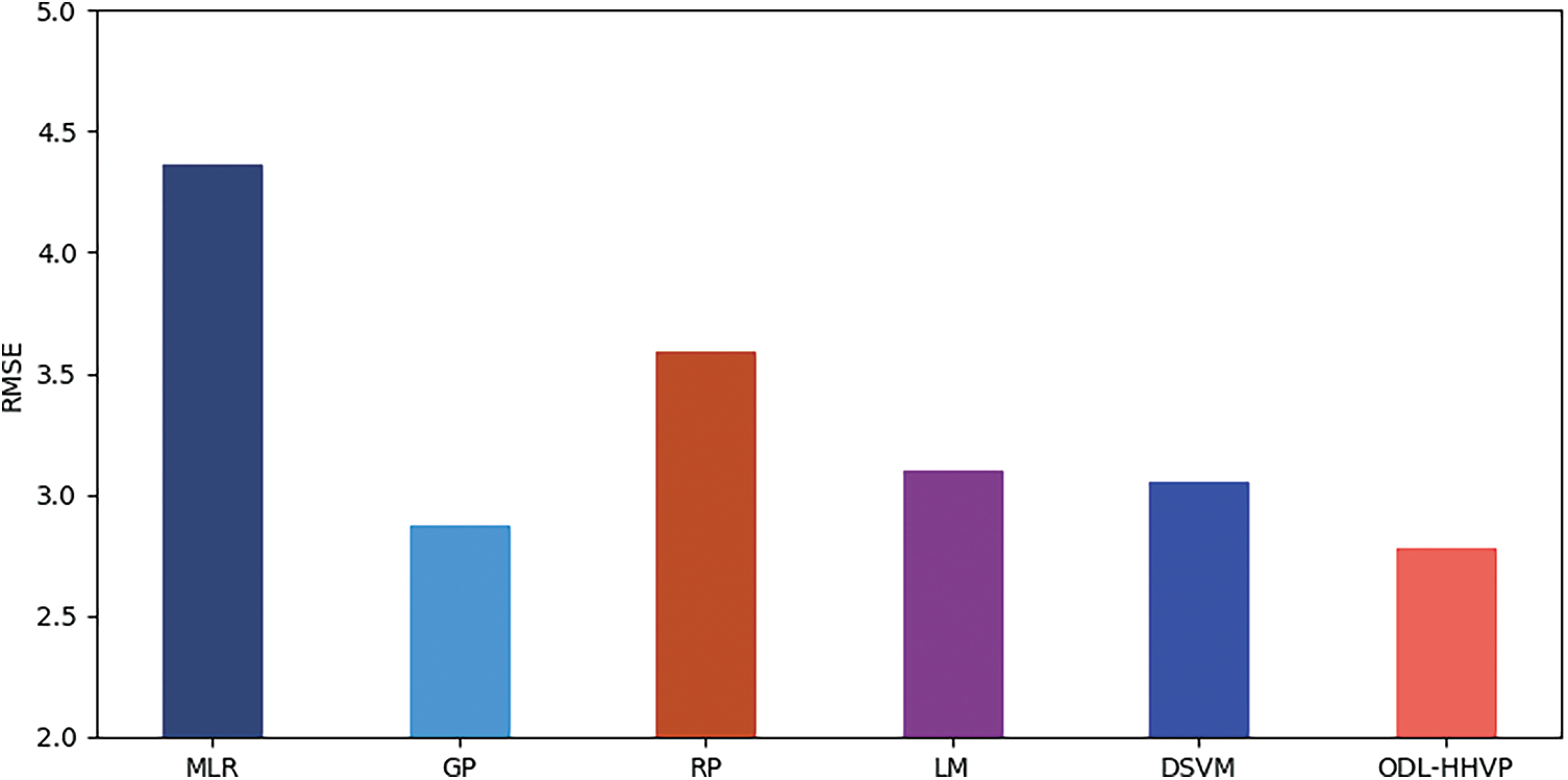
Figure 6: RMSE (Root Mean Square Error) analysis of ODL-HHVP model
Fig. 7 compares the ODL-HHVP method’s MAD analysis to that of other approaches. The graph demonstrates that the ODL-HHVP approach produces a successful outcome with a MAD of 0.294, but the RP, LM and DSVM procedures provide less successful outcomes with MADs of 2.410, 0.330 and 0.300, respectively.
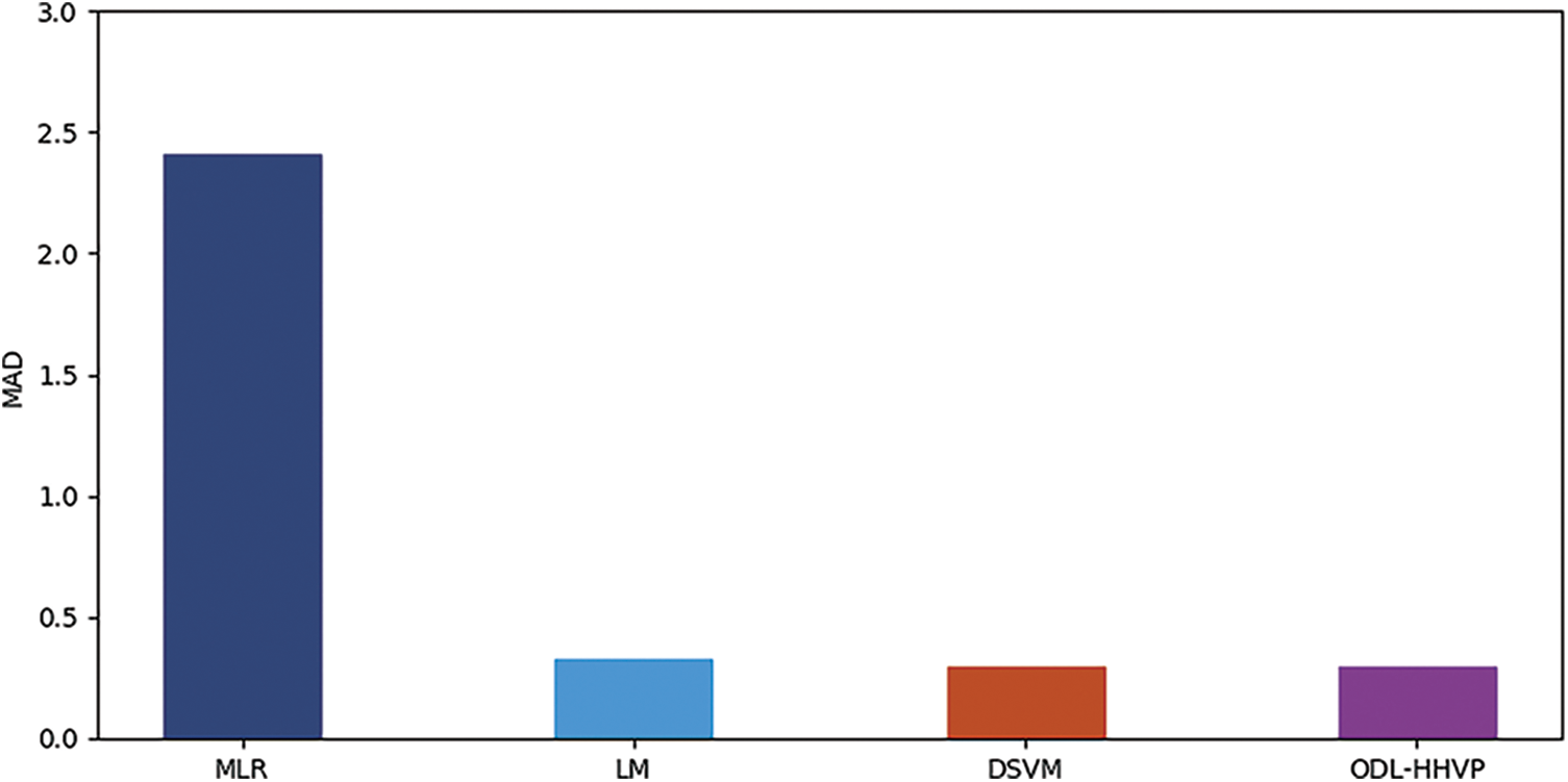
Figure 7: MAD analysis of ODL-HHVP model
Fig. 8 depicts a comparison between the MAPE analysis of the ODL-HHVP technique and earlier models. The ODL-HHVP approach had the highest MAPE at 37.410 percent, followed by the RP, LM and DSVM methods with MAPEs of 21.680%, 22.4800% and 34.560%, respectively.
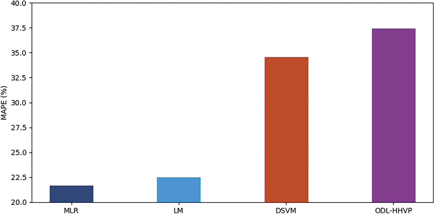
Figure 8: MAPE (Mean Absolute Percentage Error) analysis of ODL-HHVP model
Fig. 9 depicts a CC analysis of the ODL-HHVP strategy with contemporary approaches. The graph demonstrates that the ODL-HHVP approach has the greatest CC with 0.995, while the MLR, GP, RP and LM methods have the lowest CC with 0.948, 0.972, 0.988 and 0.991, respectively.
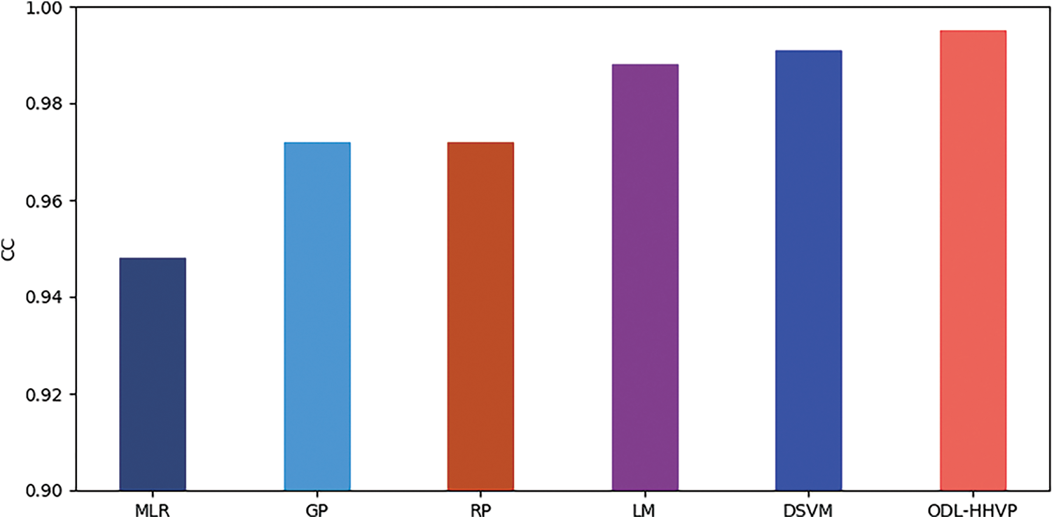
Figure 9: CC analysis of ODL-HHVP model
Tab. 4 and Fig. 10 display the deviation analysis of the ODL-HHVP in a variety of experiments employing established approaches [31–34]. The deviation value should be as low as feasible for best performance. The ODL-HHVP approach provides a deviation of 0.280 for experiment 17.960, whereas the methods of Kathiravale et al., Meraz et al., Shi et al., RP, LM and DSVM yield deviations of 4.204, 2.841, 2.710, 3.991, 0.346 and 0.315, respectively. In addition, for the 16.050 experiment, the ODL-HHVP technique yields the smallest deviation of 0.004, whereas the Kathiravale et al., Meraz et al., Shi et al., RP, LM and DSVM methods yield larger deviations of 3,391, 3,107, 3,134, 12,480, 0.008 and 0.007, respectively. In addition, for the 9.960 experiment, the ODL-HHVP approach yields a deviation of 0.181, whereas the methods of Kathiravale et al., Meraz et al., Shi et al., RP, LM and DSVM provide deviations of 9.213, 5.374, 9.898, 3.096 0.227 and 0.221, respectively. Consequently, the ODL-HHVP method produces a deviation of 0.004 for experiment 5.691, whereas the Kathiravale et al., Meraz et al., Shi et al., RP, LM and DSVM methods yield deviations of 0.210, 0.152, 16.786, 2.254, 0.056 and 0.042, respectively.
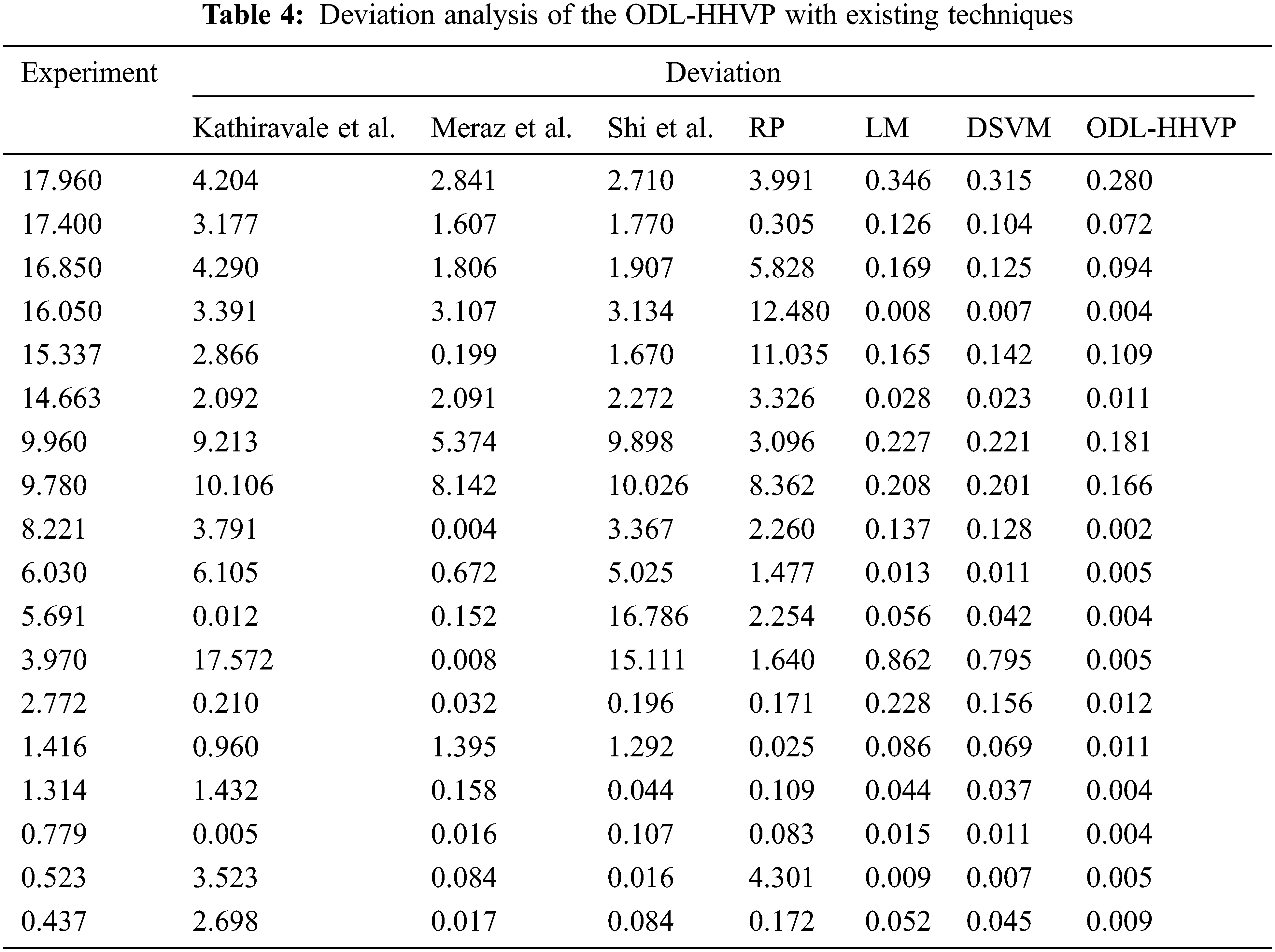
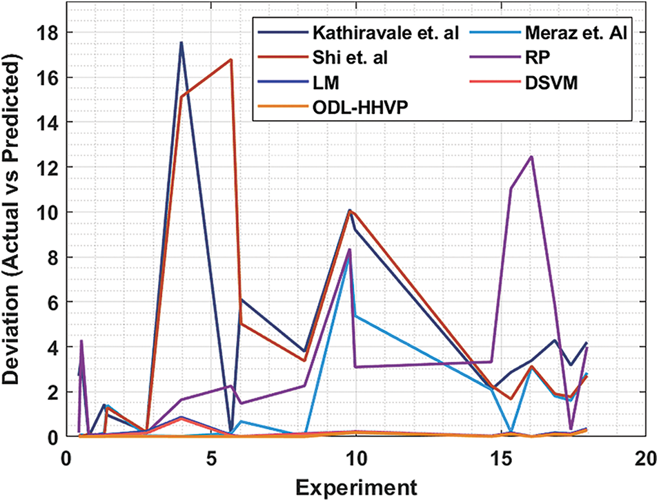
Figure 10: Deviation analysis of ODL-HHVP with existing techniques
In accordance with the experiment, the ODL-HHVP approach has a 0.004 deviation, whereas Kathiravale et al., Meraz et al., Shi et al., RP, LM and DSVM had maximum deviations of 1.432, 0.158, 0.109, 0.044 and 0.037, respectively. The ODL-HHVP method produces a minimal deviation of 0.009 with an experiment of 0.437, whereas the methods of Kathiravale et al., Meraz et al., Shi et al., RP, LM and DSVM achieve deviations of 2.698, 0.017, 0.1721, 0.052 and 0.045, respectively.
Using the contents of oxygen, water, hydrogen, carbon, nitrogen, sulphur and ash, the purpose of this research is to create a new ODL-HHVP approach for determining the HHV value in MSW management. Using the ODL-HHVP method, the DSVM model was developed as a regression strategy for determining the HHV value in MSW management. In addition, by utilising the BSO technique to optimise the DSVM model’s parameters, the prediction performance and MSE are significantly enhanced. To show the enhanced performance of the ODL-HHVP approach, a number of simulations are executed and the generated data is evaluated on a variety of levels. The experimental findings demonstrated that the ODL-HHVP method outperforms the present state-of-art methods. Therefore, the ODL-HHVP method may be applied to accurately predict HHV. Enhanced DL models with hybrid Meta techniques for parameter optimization can be developed in future to improve the performance of HHV prediction.
Funding Statement: The authors received no specific funding for this study.
Conflicts of Interest: The authors declare that they have no conflicts of interest to report regarding the present study.
References
1. G. H. Nordi, R. Palacios-Bereche, A. G. Gallego and S. A. Nebra, “Electricity production from municipal solid waste in Brazil,” Waste Management & Research, vol. 35, no. 7, pp. 709–720, 2017. [Google Scholar]
2. H. Cheng and Y. Hu, “Municipal solid waste (MSW) as a renewable source of energy: Current and future practices in China,” Bioresource Technology, vol. 101, no. 11, pp. 3816–3824, 2010. [Google Scholar]
3. N. Subramani and D. Paulraj, “A gradient boosted decision tree-based sentiment classification of twitter data,” Intl. Journal of Wavelets, Multiresolution and Information Processing, vol. 18, no. 4, pp. 1–15, 2020. [Google Scholar]
4. P. Kasar and M. Ahmaruzzaman, “Correlative HHV prediction from proximate and ultimate analysis of char obtained from co-cracking of residual fuel oil with plastics,” Korean Journal of Chemical Engineering, vol. 38, no. 7, pp. 1370–1380, 2021. [Google Scholar]
5. Y. Maksimuk, Z. Antonava, V. Krouk, A. Korsakova and V. Kursevich, “Prediction of higher heating value based on elemental composition for lignin and other fuels,” Fuel, vol. 263, pp. 116727, 2020. [Google Scholar]
6. R. Amen, J. Hameed, G. Albashar, H. W. Kamran, M. U. H. Shah et al., “Modelling the higher heating value of municipal solid waste for assessment of waste-to-energy potential: A sustainable case study,” Journal of Cleaner Production, vol. 287, pp. 125575, 2021. [Google Scholar]
7. I. Estiati, F. B. Freire, R. Aguado and M. Olazar, “Fitting performance of artificial neural networks and empirical correlations to estimate higher heating values of biomass,” Fuel, vol. 180, pp. 377–383, 2016. [Google Scholar]
8. Q. Li, Y. Long, H. Zhou, A. Meng and Z. Tan, “Prediction of higher heating values of combustible solid wastes by pseudo-components and thermal mass coefficients,” Thermochimica Acta, vol. 658, pp. 93–100, 2017. [Google Scholar]
9. H. Shi, N. Mahinpey, A. Aqsha and R. Silbermann, “Characterization, thermochemical conversion studies and heating value modeling of municipal solid waste,” Waste Management, vol. 48, pp. 34–47, 2016. [Google Scholar]
10. P. Mohan and R. Thangavel, “Resource selection in grid environment based on trust evaluation using feedback and performance,” American Journal of Applied Sciences, vol. 10, no. 8, pp. 924–930, 2013. [Google Scholar]
11. W. Li, K. C. Loh, J. Zhang, Y. W. Tong and Y. Dai, “Two-stage anaerobic digestion of food waste and horticultural waste in high-solid system,” Applied Energy, vol. 209, pp. 400–408, 2018. [Google Scholar]
12. S. Neelakandan and R. Annamalai, “Efficient solution to the waste management process using iot for smart trash can,” Journal of Emerging Technologies and Innovative Research, vol. 5, no. 6, pp. 32–40, 2018. [Google Scholar]
13. I. Boumanchar, Y. Chhiti, F. E. M. H. Alaoui, M. Elkhouakhi, L. Deshayes et al., “Thermo-chemical behavior of biomass, coal, municipal solid wastes and their mixtures,” in 2020 5th Int. Conf. on Renewable Energies for Developing Countries (REDEC), Morocco, pp. 1–5, 2020. [Google Scholar]
14. C. Saravanakumar, R. Priscilla, B. Prabha, A. Kavitha and C. Arun, “An efficient on-demand virtual machine migration in cloud using common deployment model,” Computer Systems Science and Engineering, vol. 42, no. 1, pp. 245–256, 2022. [Google Scholar]
15. R. Krishnan, L. Hauchhum, R. Gupta and S. Pattanayak, “Prediction of equations for higher heating values of biomass using proximate and ultimate analysis,” in 2018 2nd Int. Conf. on Power, Energy and Environment: Towards Smart Technology (ICEPE), State Convention Center (Pine Wood Hotel Annex) European Ward, Rita Road, Shillong, Meghalaya 793001, pp. 1–5, 2018. [Google Scholar]
16. S. Neelakandan and D. Paulraj, “An automated exploring and learning model for data prediction using balanced CA-SVM,” Journal of Ambient Intelligence and Humanized Computing, vol. 12, no. 5, pp. 4979–4990, 2021. [Google Scholar]
17. B. Jaishankar, S. Vishwakarma, S. P. Aditya Kumar and N. Arulkumar, “Blockchain for securing healthcare data using squirrel search optimization algorithm,” Intelligent Automation & Soft Computing, vol. 32, no. 3, pp. 1815–1829, 2022. [Google Scholar]
18. I. Boumanchar, Y. Chhiti, F. E. M’hamdi Alaoui, A. Sahibed-Dine, F. Bentiss et al., “Municipal solid waste higher heating value prediction from ultimate analysis using multiple regression and genetic programming techniques,” Waste Management & Research, vol. 37, no. 6, pp. 578–589, 2019. [Google Scholar]
19. B. P. Sankaralingam and K. K. Dhawan, “Fault tolerance-genetic algorithm for grid task scheduling using check point,” in IEEE Sixth Int. Conf. on Grid and Cooperative Computing, China, pp. 676–680, 2007. [Google Scholar]
20. D. O. Melinte, A. M. Travediu and D. N. Dumitriu, “Deep convolutional neural networks object detector for real-time waste identification,” Applied Sciences, vol. 10, no. 20, pp. 7301, 2020. [Google Scholar]
21. Y. Alotaibi, S. Alghamdi, O. Khalaf and U. Sakthi, “Improved metaheuristics-based clustering with multihop routing protocol for underwater wireless sensor networks,” Sensors, vol. 22, no. 4, pp. 1618, 2022. [Google Scholar]
22. M. Prakash and T. Ravichandran, “An efficient resource selection and binding model for job scheduling in grid,” European Journal of Scientific Research, vol. 81, no. 4, pp. 450–458, 2012. [Google Scholar]
23. J. O. Ighalo, A. G. Adeniyi and G. Marques, “Application of linear regression algorithm and stochastic gradient descent in a machine learning environment for predicting biomass higher heating value,” Biofuels, Bioproducts and Biorefining, vol. 14, no. 6, pp. 1286–1295, 2020. [Google Scholar]
24. H. Li, Q. Xu, K. Xiao, J. Yang, S. Liang et al., “Predicting the higher heating value of syngas pyrolyzed from sewage sludge using an artificial neural network,” Environmental Science and Pollution Research, vol. 27, no. 1, pp. 785–797, 2020. [Google Scholar]
25. S. Pattanayak, L. Hauchhum and L. Sailo, “Application of MLP-ANN models for estimating the higher heating value of bamboo biomass,” Biomass Conversion and Biorefinery, vol. 11, no. 6, pp. 2499–2508, 2021. [Google Scholar]
26. M. Cubillos, “Multi-site household waste generation forecasting using a deep learning approach,” Waste Management, vol. 115, pp. 8–14, 2020. [Google Scholar]
27. M. Prakash, R. Farah Sayeed, S. Princey and S. Priyanka, “Deployment of multicloud environment with avoidance of ddos attack and secured data privacy,” International Journal of Applied Engineering Research, vol. 10, no. 9, pp. 8121–8124, 2015. [Google Scholar]
28. M. Sundaram, S. Satpathy and S. Das, “An efficient technique for cloud storage using secured de-duplication algorithm,” Journal of Intelligent & Fuzzy Systems, vol. 42, no. 2, pp. 2969–2980, 2021. [Google Scholar]
29. J. Deepak Kumar and S. T. Sumarga Kumar, “Metaheuristic optimization-based resource allocation technique for cybertwin-driven 6G on ioe environment,” IEEE Transactions on Industrial Informatics, vol. 18, no. 7, pp. 4884–4892, 2022. [Google Scholar]
30. P. Singh, A. Kaur, R. S. Batth, S. Kaur and G. Gianini, “Multi-disease big data analysis using beetle swarm optimization and an adaptive neuro-fuzzy inference system,” Neural Computing and Applications, vol. 33, no. 16, pp. 10403–10414, 2021. [Google Scholar]
31. O. O. Olatunji, S. Akinlabi, N. Madushele and I. Felix, “Multilayer perceptron artificial neural network for the prediction of heating value of municipal solid waste,” AIMS Energy, vol. 7, no. 6, pp. 944–956, 2019. [Google Scholar]
32. S. Kathiravale, M. N. M. Yunus, K. Sopian, A. H. Samsuddin and R. A. Rahman, “Modeling the heating value of municipal solid waste,” Fuel, vol. 82, no. 9, pp. 1119–1125, 2013. [Google Scholar]
33. M. A. Berlin, S. Tripathi, V. B. Devi, I. Bhardwaj, N. Subramani et al., “IoT-Based traffic prediction and traffic signal control system for smart city,” Soft Computing, vol. 25, no. 18, pp. 12241–12248, 2021. [Google Scholar]
34. L. Meraz, A. Domı́nguez, I. Kornhauser and F. Rojas, “A thermochemical concept-based equation to estimate waste combustion enthalpy from elemental composition,” Fuel, vol. 82, no. 12, pp. 1499–1507, 2003. [Google Scholar]
Cite This Article
 Copyright © 2023 The Author(s). Published by Tech Science Press.
This work is licensed under a Creative Commons Attribution 4.0 International License , which permits unrestricted use, distribution, and reproduction in any medium, provided the original work is properly cited.
 Downloads
 Citation Tools