Precise Multi-Class Classification of Brain Tumor via Optimization Based Relevance Vector Machine

1  Introduction

Image processing is the system to carry out various processes on the images, to get better images as an output, or to dig out some valuable data from it [1]. It takes an input in the form of an image and produces an image as an output, or any characteristics or features associated with that image as an output. The term “brain tumor” refers to a mass of aberrant brain cells that have developed abnormally. Some of the brain tumors are non-cancerous (benign) and others are cancerous (malignant). Computed Tomography (CT), MRI, Angiography, and Skull X-ray are the different modes to identify the tumors. This study is primarily concerned with digital images, which are sometimes known as pixels or groups of pixels, and which have finite or discrete numeric representations of intensity or grey levels [2] that are regarded because of their two-dimensional functions, which are provided as input by its spatial coordinates, indicated by the letters x and y [3]. The basic phases in image processing include Image acquirement, Image enrichment, Color-image processing, morphological, segmentation, Object identification, Wavelets, and multi-resolution and compression [4].

Every year, around 350,000 new instances of brain tumors are discovered across the globe. According to the International Association of Cancer Registries (IARC) in India, more than 1,28, 000 reported cases and 1,21,345 died due to brain tumors. There are various challenges in detecting and diagnosing the tumor as it requires detailed clinical information regarding tumor location, type, and growth speed [5]. This leads to the correct diagnosis and further treatment. The next challenge is that there are no well-defined segmentation algorithms because it’s hard to define the borders of objects. People with cancer of the brain or Central Nervous System (CNS) have a maximum 5-year survival rate of 36% [6]. This paper is going to consider the above challenges as the problem statement. This paper mainly focuses on preprocessing, segmentation, feature selection, and extraction and classification within the application of biomedical image processing and mainly in the area of brain tumors. The brain is a crucial component of the human central nervous system, containing 50–100 billion neurons and forming a massive network structure.

Image processing plays a vital role in various fields. It is mainly used in the medical field for diagnosing various diseases, especially in the brain. They are invasive and are of high resolution. Most imaging tests are used to diagnose a brain tumor. There are different techniques available for diagnosing brain tumors such as Magnetic Resonance Imaging (MRI) scan, Computed Tomography (CT or CAT) scans, Positron Emission tomography, and X-rays. Each of these modalities provides different information about the brain. A positron emission tomography (PET) scan is used to find more about a tumor while a patient is receiving treatment or if the tumor comes back after treatment. The most effective and commonly used tool is the MRI scan. It produces a detailed image of the body and also it is used to measure the size of the tumor. Since, the tumors may vary in size, shape, and location day by day. It has high spatial resolution and high soft-tissue contrast. It does not use any harmful ionizing radiation like a CT scan. The visual evaluation and examination of MRI images by radiologists leads to some difficulties and also may cause errors. Because of its high clinical relevance and its challenging nature, the problem of computational brain tumor segmentation has paved the way for many algorithmic approaches for automated, semi-automated, and interactive segmentation of tumor structures.

In this paper, an algorithmic image processing technique is proposed that can help radiologists diagnose the tumor automatically in multi-parametric MR images since brain tumor detection and segmentation needs to take into account large variations in the appearance and shape of structures. So, we need automated systems for the analysis and classification of the images.

The remainder of this article is organized into five sections. Section 2 discusses the existing techniques analysis. Section 3 provides detailed information about the proposed methodology for the multi-class classification of brain tumors. Section 4 discusses the experimental results and finally, Section 5 concludes the findings of the proposed work with future enhancement.

2  Related Work

There are several algorithms presented in the literature for brain tumor detection. Tab. 1 illustrates the exhaustive study of the existing works on pre-processing, segmentation, feature selection, extraction, and categorization. Moreover, the results of each technique are also discussed in detail.

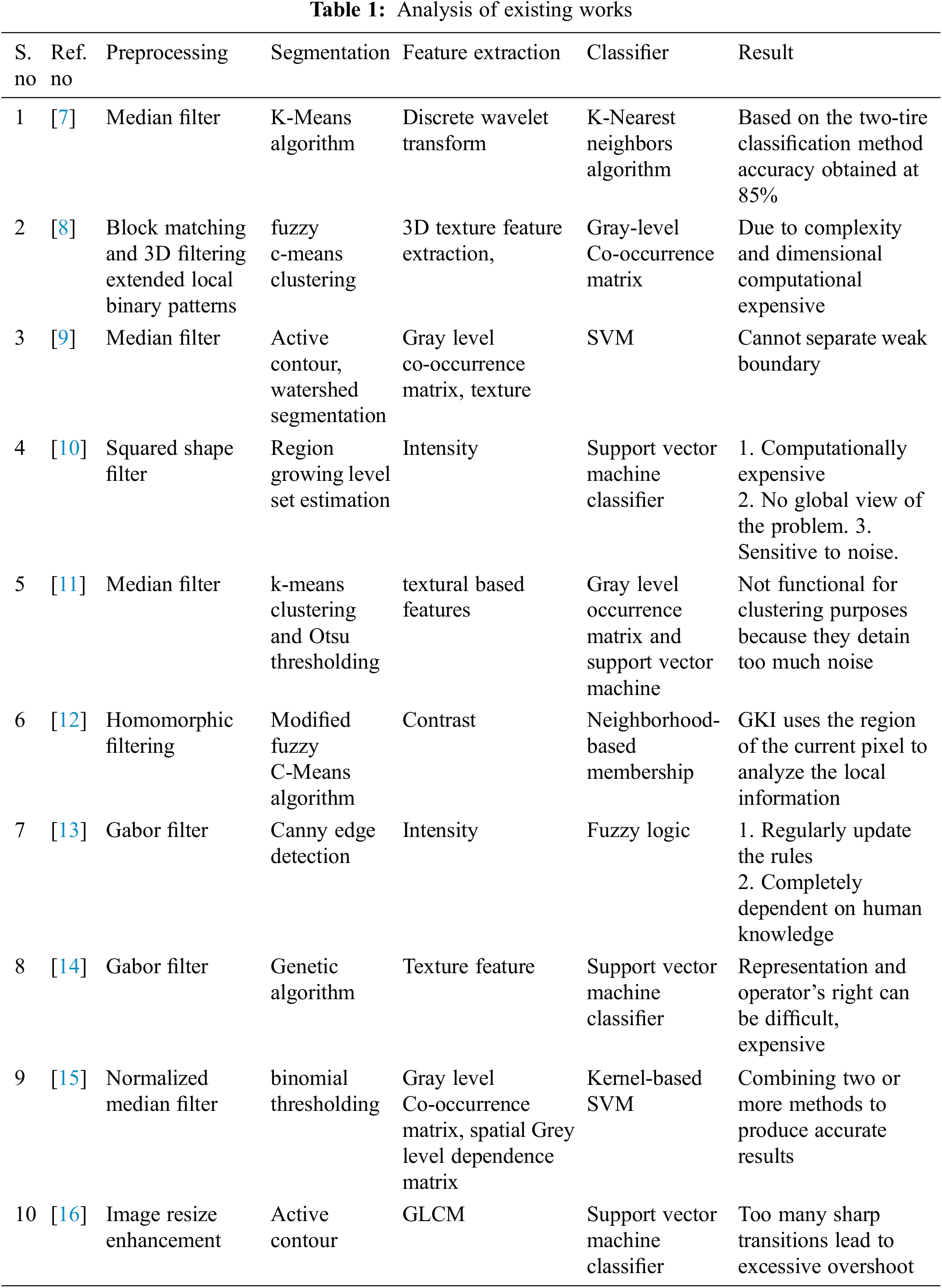
There are several obstacles to image segmentation and classification, such as creating a standardized model that can be extended to all forms of images and purposes. However, choosing the right technique for a particular type of image is a difficult problem. Therefore, for the identification and classification of images, there is no broadly agreed procedure. In the field of computer vision systems, it remains a major obstacle. The approach failed to consider classifying images of various pathological disorders, types, and status of the disease. The system includes a lot of pure nodes that can result in overfitting. Designers suggested a Machine learning and optimization principle to accomplish an automated brain tumor identification using brain MRI images and to evaluate its efficiency to overcome these problems.

3  Relevance Vector Machine Brain Classification

This paper describes the various materials used to bring together and extract the data from brain MRI. The major purpose of this paper is to formulate a methodology for the extraction of features and segments from the data. To produce an accurate result, the MRI images were used in this paper. The schematic architecture of the proposed RVM is depicted in Fig. 1. The preprocessing process is used to get rid of the noise from the input image. After that, segmentation and feature extraction will be performed, and the outcome will be given to the classifier to find out if the sample is affected or not.

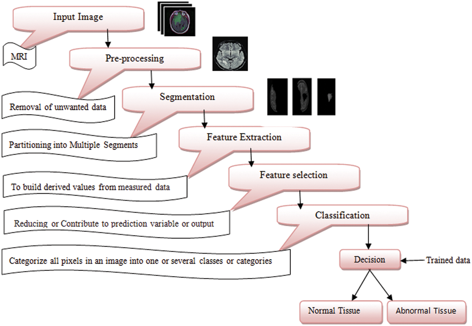
Figure 1: Schematic architecture of proposed RVM for multi-class classification

3.1 Data Set

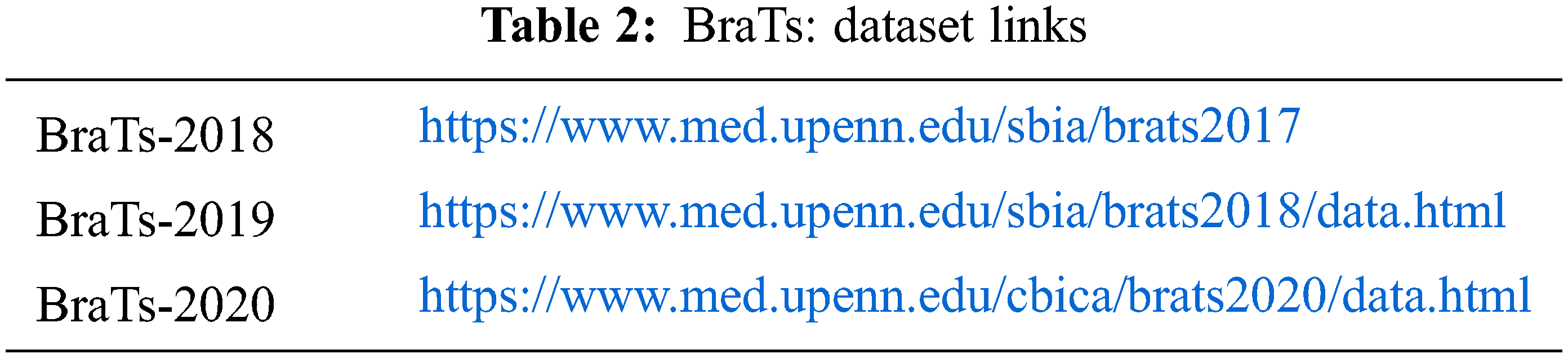
This dataset is provided by Medical image computing and computer-assisted intervention (MICCAI). This is one of the authorized databases for segmenting such brain MRI images as a challenge, and researchers have extensively used it for MRI brain tumor image segmentation [17]. The BraTs databases have been restructured every year since the challenge began in 2012. Tab. 2 BraTs dataset following is the URL for the BraTs database referenced in this paper.

3.2 Image Preprocessing

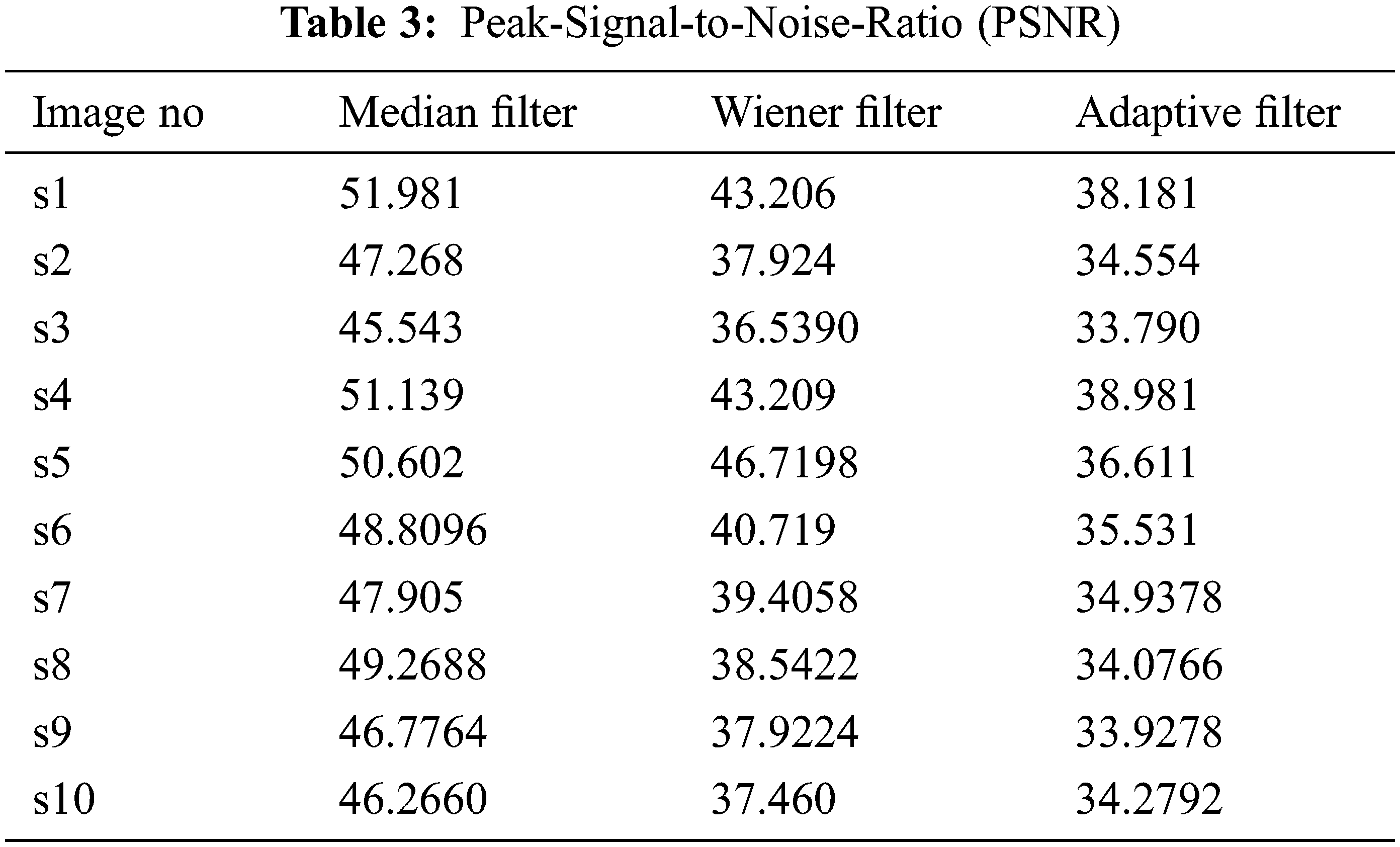
The preprocessing technique used reduces the complexity and increases the accuracy and is also used to reconstruct the image. It converts the binary image to the gray scales (black and white). MRI is one of the most highly developed full-concept imaging modalities for cancer treatment. Getting an accurate MRI is a big challenge because of the Gaussian noise and the speckle noise. The exact brain image is essential for further diagnosis processing [18]. According to, the performance of the filter is evaluated from the PSNR (peak signal-to-noise ratio) value like Tab. 3.

A=10log10(MAX12X) (1)

Eq. (1) is further reduced into Eq. (2) to increase the performance of the machine and used to decrease the computational point in time.

A=log((MaxPixel)/√x) (2)

where the (2) equation represents

X is the mean-square error and collective squared error among the squashed and the new image.

A is the peak-signal-to-noise ratio and is a measure of the peak error.

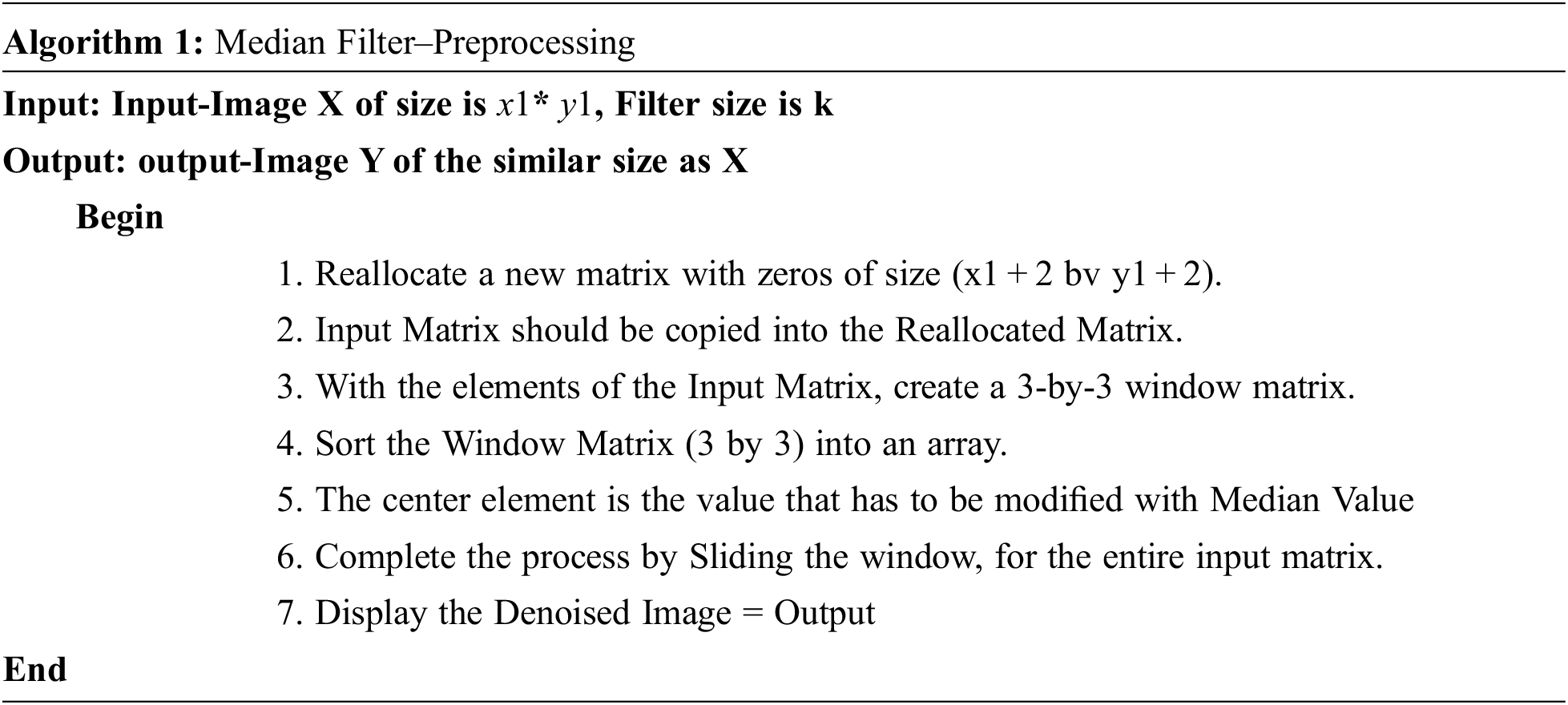
The median filter is the best and high efficient performing filter on comparing with the wiener and adaptive filter [18]. The Median filter is mainly used for smoothening effect particularly best to remove the speckle noise and also it is used to reduce the intensity variation. Median filter for one dimensional let us consider the pixel value a = (2, 3, 80, 6, 2, 3).

As a result, y will be the median filtered output signal:

Ya = med (1, 6, 80) = 6,

Yb = med (2, 80, 4) = med (2, 4, 80) = 4,

Yc = med (70, 6, 1) = med (1, 6, 70) = 6,

Yd = med (4, 1, 3) = med (1, 3, 64) = 3,

Then the output of b = (6, 4, 6, 3).

This paper is based on a two-dimensional image shown in Fig. 2.

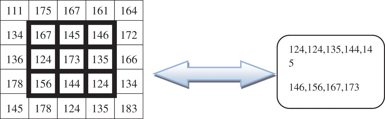
Figure 2: Two-dimensional images

Therefore, the formula is

f^˙(x1, y1)=median(a,b) ∈ sx1,y1{ g(a, b) }(3)

Eq. (3) is used to calculate the median value by restoring the gray level of every pixel by the median of the gray levels in a region of the pixels, in its place of using the average operation. Fig. 3a the Original image input image for the system and Fig. 3b is the Pre-Processed image as the output of the process

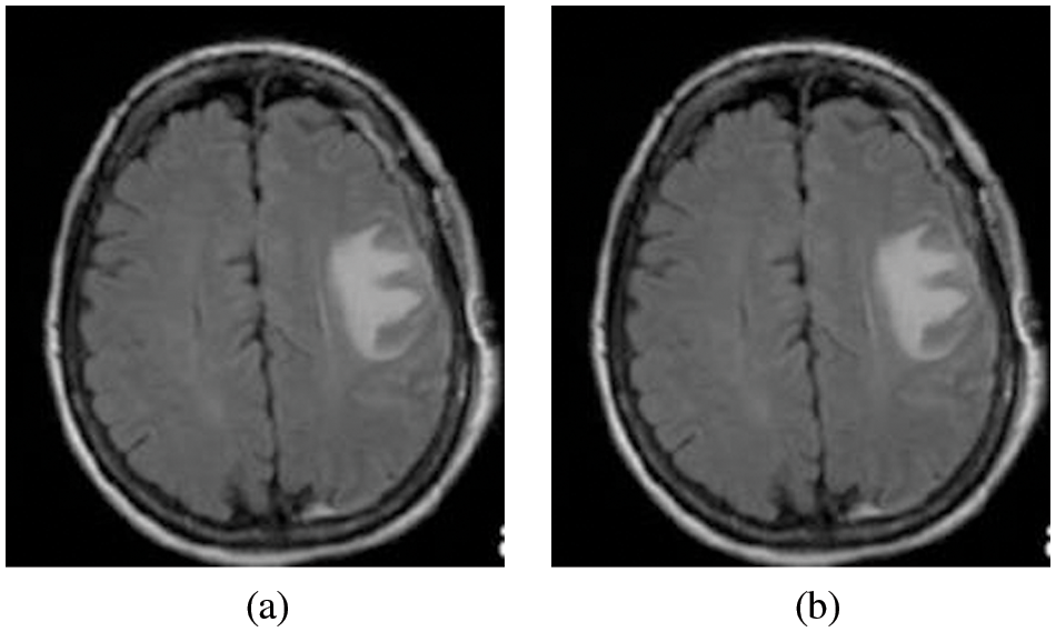
Figure 3: (a) Original image and (b) Pre-processed image

Skull stripping is a crucial practice in brain representation analysis. Skull-stripping or scalp editing to eradicate non-brain areas earlier than normalizing brains, even though this is important to all the normalization techniques [19]. Fig. 4a Pre-Processed image as the input for the skull stripping and Fig. 4b is the Image after skull stripping.

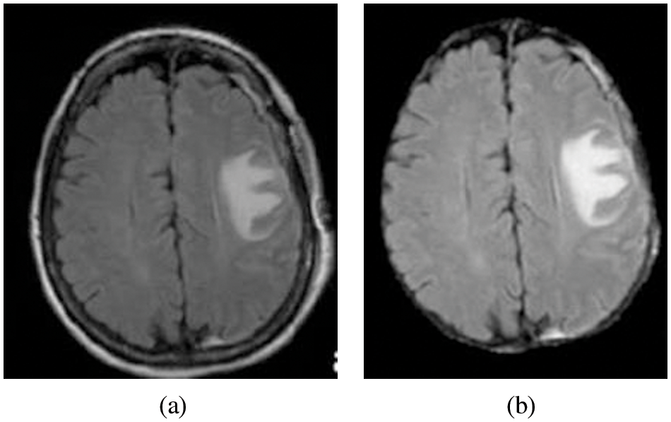
Figure 4: (a) Pre-processed image (b) Image after skull stripping

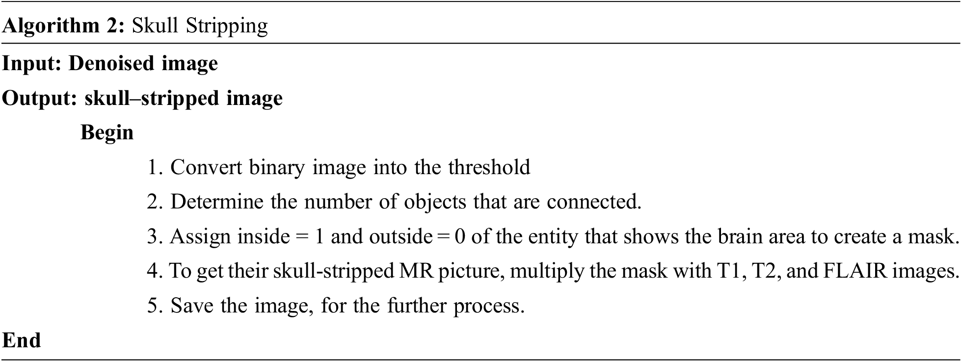
Now, fill in the image by sealing off the absolute bottom of the top. Skull stripping can be done using intensity-based, morphology-based, deformable surface-based, hybrid approaches, or atlas-based. Brain structure and size are not standardized and differ from person to person. This is the main challenge of skull stripping; it also helps to get better speed and accuracy.

3.3 Image Segmentation

Image segmentation is a digital image splitting technique that divides a digital image into multiple sections as a subset in Eq. (4). Segmentation makes it easier for people to interpret an image by decreasing and/or changing its representation. Segmentation methods are employed to separate the necessary items from the picture for object analysis. The technique of conveying a label of each pixel in the images such that the pixel in the image has related properties like Fig. 5 is known as the segmentation process.

ImageA⊆ImageB (4)

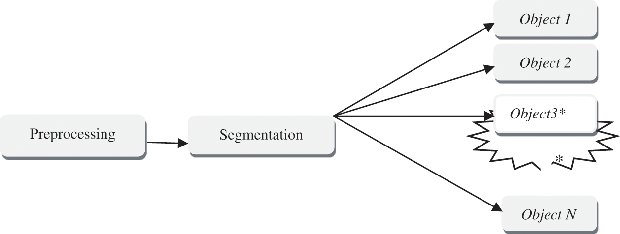
Figure 5: Segmentation process

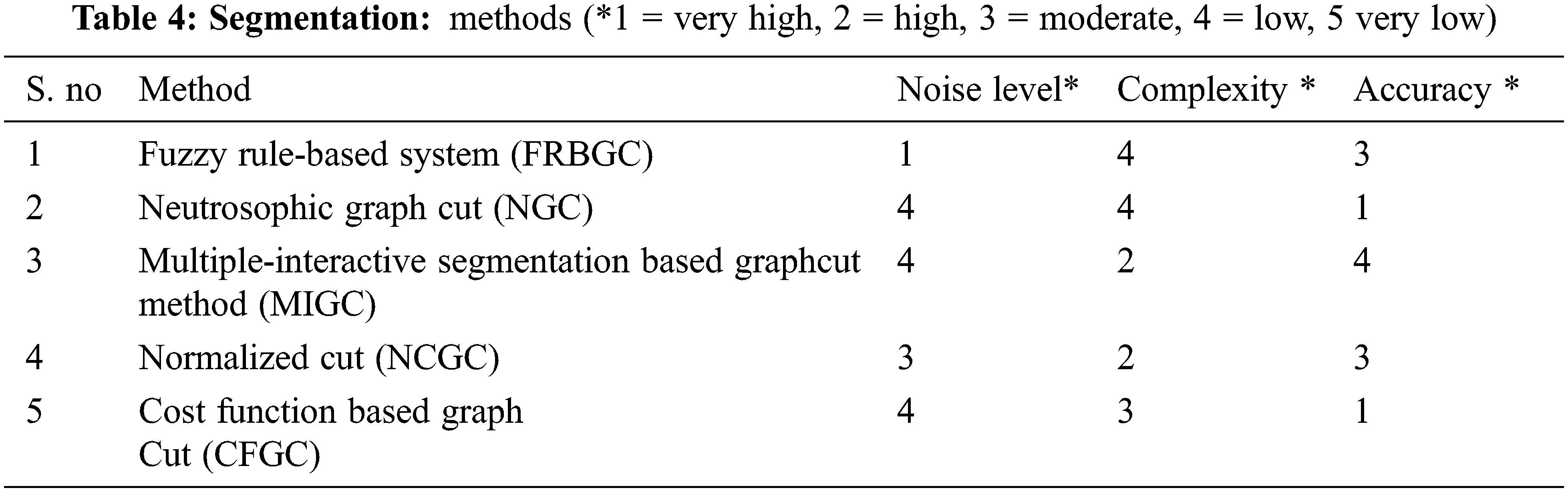
Graph cuts are used to partition grayscale, color, and textured pictures in a fuzzy rule-based system. This system is meant to discover the weight that should be assigned to a certain image characteristic during graph construction, depending on the types of the picture. The normalized graph generated from the fuzzy rule-based weighting factor of several picture characteristics is then employed.

The proposed method Neutrosophic graph cut (NGC) [20] developed an effective picture segmentation technique as compared in Tab. 4. The mathematical formalism value of the output picture is referred to by integrating the intensity and spatial knowledge, and an indeterminacy filter is created using the indeterminacy characteristics of the input image. The indeterminacy kernel lowers the spatial & intensity data and information indeterminacy. Also, because the indeterminacy knowledge in the picture has been appropriately managed in the suggested technique, the findings revealed that the provided technique can split the images clearly and efficiently on both noisy and clean images.

The following are some of the novel features of the proposed method:

•   To eliminate the image’s unclear information, an indeterminate filter is proposed.

•   In the Neutrosophic domain, a new power function in the graph model has been developed and is being utilized to better segment the picture.

To separate the objects from the background, a graph cut theory algorithm is applied. Its efficiency has been examined to that of a Neutrosophic similarity clustering (NSC) segmentation method and a graph-cut-based technique in several trials [20]. The outcomes prove that the hybrid NGC method achieves better primary and secondary data outcomes.

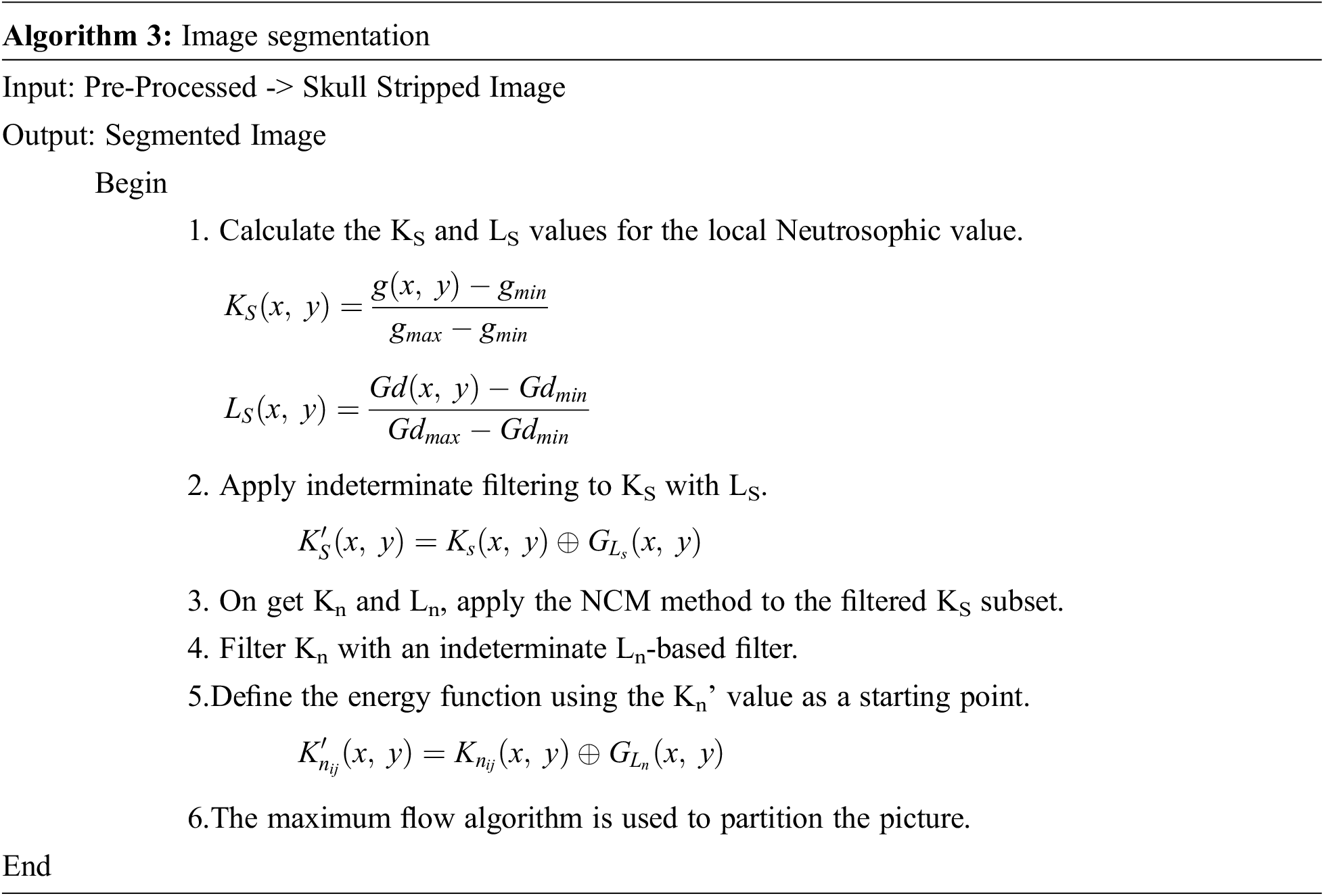
where

Ls(x, y) and Fs(x, y) denote the membership belonging to the foreground, indeterminate set, and background, respectively.

g(x, y) and Gd(x, y) are the intensity and gradient magnitude at the pixel of (x, y) on the images.

3.4 Image Feature Extraction

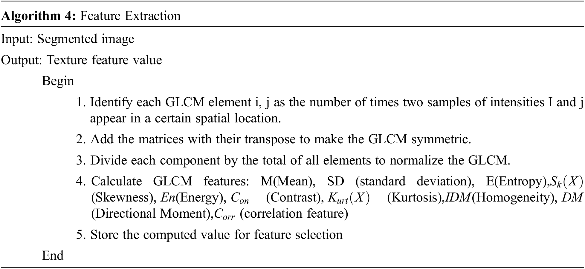
Extraction of features is a type of background subtraction in which a large number of pixels in an image are efficiently recorded so that significant sections of the image can be extracted. The texture is a property that is used to divide, and its standard is a set, into regions of interest. In an image, texture offers information about the surface distribution of colors at various intensities. The spatial pattern of time intervals in a neighborhood defines the texture.

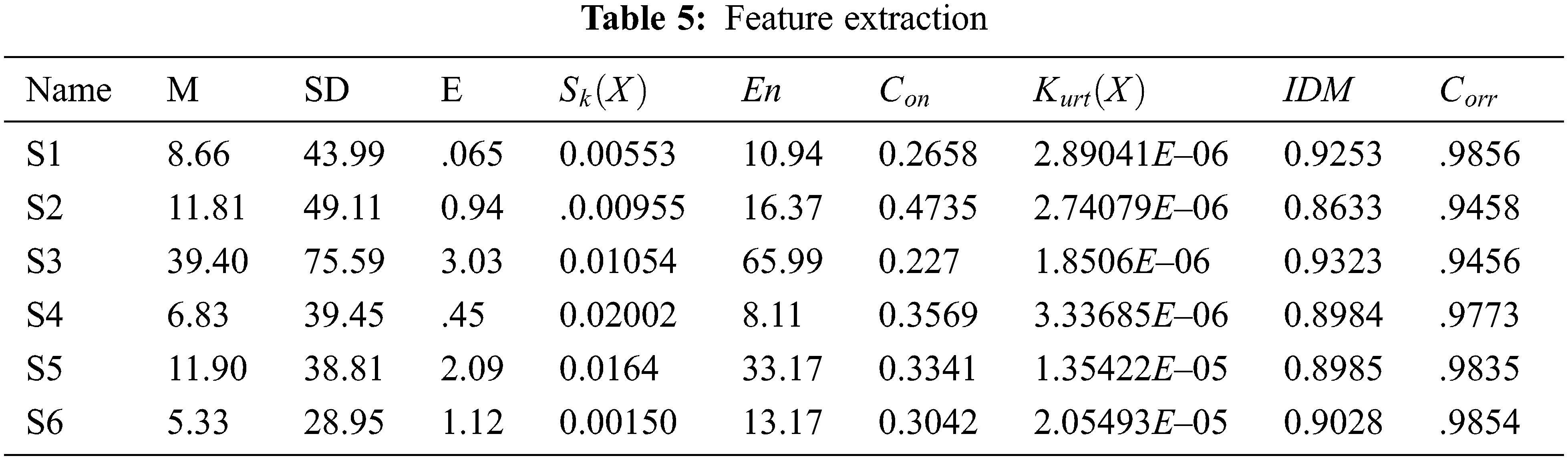
The Gray Level Co-occurrence Matrix (GLCM) analysis is a tool for obtaining statistical texture characteristics of second order. Third and higher-level textures examine the relationships between three or even more pixels, and have been employed in a variety of applications. As a result, the number of grey levels is frequently reduced [21]. The GLCM algorithms analyze how frequently an image pair of pixels with the values acquired and in a specified Euclidean distance exist, produce a GLCM, and then recover statistical metrics from the matrix to characterize an image’s texture. These attributes give information on an image’s texture [21]. Tab. 5 depicts the feature extraction results.

where,

Eq. (5) is defined as the mean of a picture is computed by multiplying all of the object’s intensity values by the entire amount of pixels in the representation.

M=(1m∗n)∑x=0m−1∑y=0n−1f(x,y) (5)

Eq. (6) is defined as the Standard deviation (SD) as the second statistical moment that describes the conditional probability of a measured population and may be used to determine in homogeneity. A greater number indicates that the image edges have a higher level of intensity and contrast.

SD=(1m∗n)∑x=0m−1∑y=0n−1(f(x,y)−M)2 (6)

Eq. (7) is defined as a term that refers to the amount of (E). Entropy is a measure of the unpredictability of a textural picture, and it is defined as

E=−∑x=0m−1∑y=0n−1f(x,y)log2f(x,y) (7)

Eq. (8) is defined Skewness as a metric for symmetry or asymmetry. Sk(X) denotes the skewness of a discrete variable X and is defined as,

Sk(X)=(1m∗n)∑(f(x,y)−M)3SD3 (8)

Eq. (9) is defined as the energy measurable amount of the extent of pixel pair repeats is referred to as energy. Energy is a metric for determining how comparable two images are. If Haralick’s GLCM characteristic is used to describe energy, it is also known as angular second instant, and it is defined as

En=∑x=0m−1∑y=0n−1f2(x,y) (9)

Eq. (10) is defined as the Contrast difference in intensity linking a pixel and its neighbor across the course of a picture.

Con=∑x=0m−1∑y=0n−1((x−y)2f(x,y)) (10)

Eq. (11) is defined as the Kurtosis as a parameter that describes the form of an unsystematic variable’s probability distribution. The Kurtosis is denoted as Kurt(X) for the random variable X and is distinct as

Kurt(X)=(1m∗n)∑(f(x,y)−M)4SD4 (11)

Eq. (12) is defined as the Homogeneity, inverse distinction. The local homogeneity of a picture is measured by its moment. To identify whether a representation is textured otherwise non-textured, IDM is may contain a single otherwise a range of values.

IDM=∑x=0m−1∑y=0n−111+(x−y)f(x,y) (12)

The spatial relationships between pixels are described by the correlation feature, which is defined as Eq. (13)

Corr=∑x=0m−1⁡∑y=0n−1⁡(x,y)f(x,y)−MXMYσXσY (13)

3.5 Feature Selection

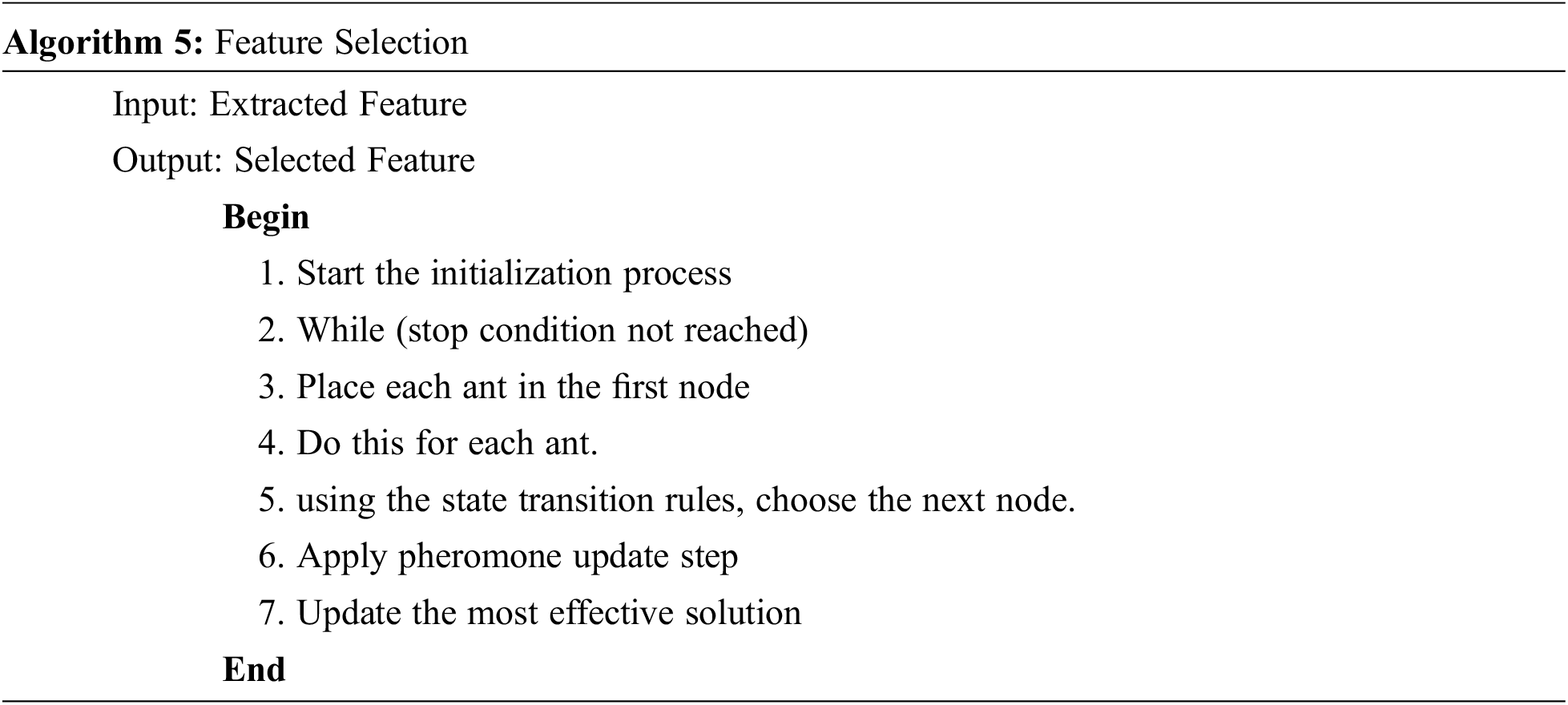
Feature selection (FS) or feature subset selection is a technique for reducing numerous features in a raw data collection by selecting relevant features and removing superfluous ones (FSS).

Ant colony optimization (ACO) is a community heuristic algorithm that may be applied to challenging optimization issues to obtain an exact solution. Artificial ants are computerized agents that look for reasonable solutions to optimization problems in ACO [22]. An Algorithm for the Ant Colony System the following are the various steps of a basic ant colony system algorithm.

1.    Problem Graph Representation

2.    Ants’ distribution Getting Started

3.    Ant’s Distribution Rule

4.    Update Global Trail

When compared to other filtering approaches, the median filter performs better. The improvement of utilizing the Median Filter is that it may eliminate the unwanted noise for preserving the edges. Ant Colony optimization is a new population-based method being proposed for the segmentation of brain tumor images. An optimization algorithm is an extremely accurate technology for forecasting.

3.6 Image Classification

Classification is the procedure designed for categorizing data into a set of categories. A classification problem’s major purpose is to determine which category/class fresh information belongs to. The relevance vector machine model is used to detect patterns. Essentially, the algorithm uses a discrimination line to separate or categories two or more different classes. The different colored dots represent different classes in this scenario and the algorithm attempts to split the groups of points with a line. If there are no points of different colors on the same side of the line, the classification method is considered successful. The RVM method divides classification into two stages. The relevance vectors are computed by the algorithm selecting a few points within each class to assist characterize the distinction line. These points define the path that the line will take between them. The chosen relative vectors are determined by taking into account all the points in the input [23,24]. The RVM method is similar to the SVM method in terms of functionality. Using simply the supports or relevance vectors, they simultaneously derive a discrimination line [25]. The distinctions are in the manner in which those vectors are formed. In the Development of science, support vectors are calculated only for selected points of the classes’ actual boundaries. The rest of the points are then ignored. In RVM learning, relevance vectors are constructed by taking into account all locations in the input [26].

4  Experimental Result Analysis

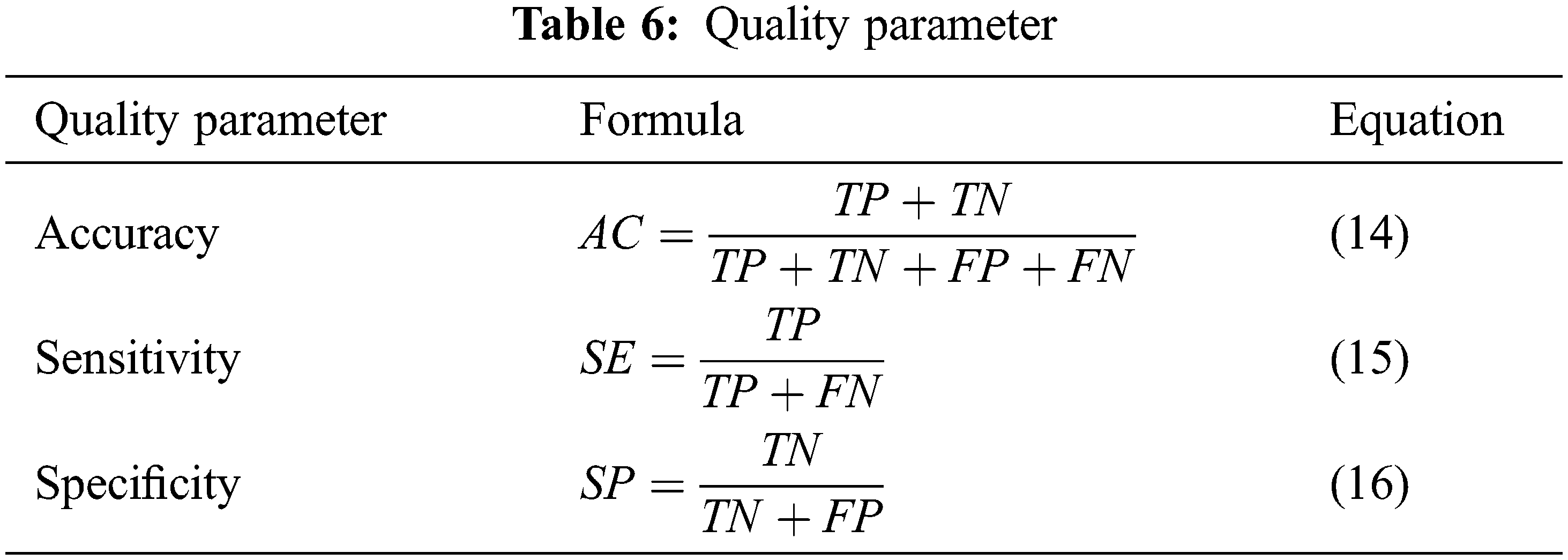
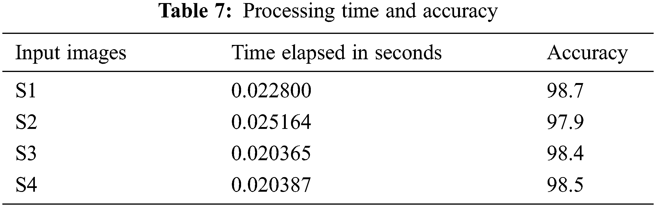
The experimental analysis is done using the MATLAB simulation tool. Performance of the system in every brain tumor MRI picture, there is some mistake rate dependent on whether aberrant tissue is detected. These may be calculated using “True Positive, False Positive, True Negative, and False Negative” numbers. All samples in the database were evaluated to determine the system’s accuracy, sensitivity, and specificity. The following four qualities are used to analyze the existing and the proposed system in accuracy, sensitivity, and specificity. Tab. 6 represents the quality parameter calculated by TP: Test result indicates that the objective deviation exists and was accurately identified. TN: The test result indicates that the objective deviation did not exist and that it was not identified appropriately. FP: Test results are positive for the absence of the objective deviation, which was accurately identified. FN: The test result was incorrectly identified and is negative for the existence of the objective deviation. Finally, the Processing Time and Accuracy are provided in Tab. 7.

The accuracy is calculated and compared to the existing model. The performance of the RVM, data validation and validation loss are computed to assess the effectiveness of the proposed brain tumor classification using the RVM technique. The current strategy for detecting brain tumors is the Support Vector Machine (SVM), which is based primarily on classification. It demands the feature extraction outcome. From the comparison graph Fig. 6, the proposed classification result is created based on the feature value, and the accuracy is estimated to be 98.87%.

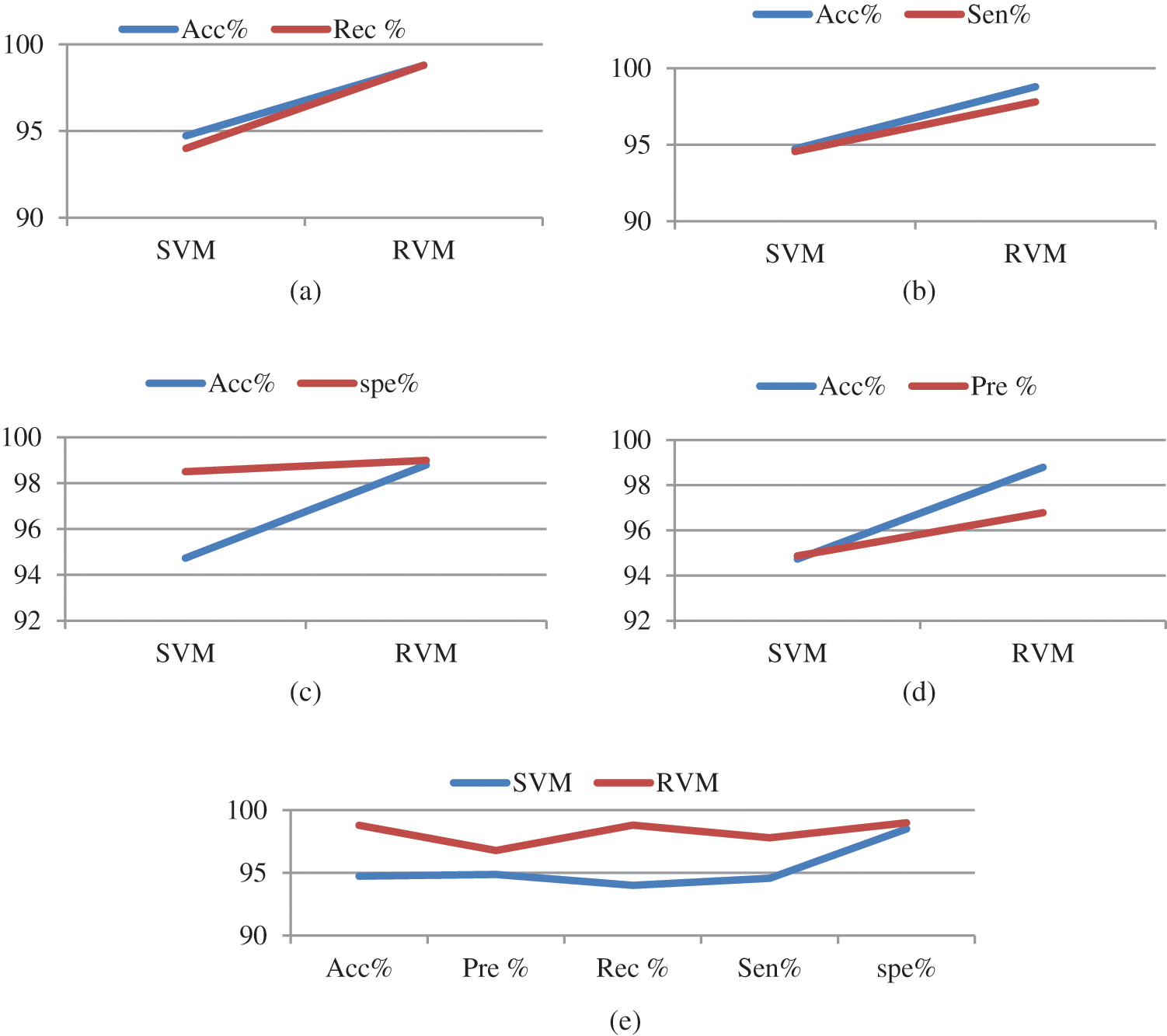
Figure 6: Comparison graph

5  Conclusion

In this paper, the relevance vector machine (RVM) is used for the multi-class classification of brain tumors as normal or anomalous. The proposed model involves pre-processing, segmentation, feature extraction, feature selection, and classification of MRI images. For the classification, the proposed RVM model uses three datasets namely Brats 2018, 2019, and 2020. The complexity and computing time are minimal, yet the accuracy of the system is greater. The graph shows the accuracy with which brain tumors are classified. Finally, the categorization sample is normal or abnormal, depending on the segmentation and classification technique. The performance of the proposed RVM technique is compared to that of the classic SVM based on the specificity, sensitivity, and accuracy rate, in which the proposed RVM technique achieves a better accuracy rate of 98.87%. As a result, the research concludes that the proposed technique distinguishes between normal and abnormal tumors and allows the clinical specialists to make more informed diagnosis decisions; this is the main advantage of the proposed system.

In future work, various classifiers can be utilized to improve accuracy by using more professional segmentation techniques and feature extraction algorithms with real-world and medical data with large datasets placed under various circumstances. In future work, we are aiming to increase the size of the dataset by including more patients of different ages, symptoms, and gender.

Acknowledgement: We express our gratitude to anonymous referees for their useful suggestions.

Funding Statement: The authors did not receive any funding for this study.

Conflicts of Interest: The authors proclaim that they have no conflicting interests to account about this study.

References

1. J. Kuruvilla, D. Sukumaran, A. Sankar and S. P. Joy, “A review on image processing and image segmentation,” in Proc. Int. Conf. on Data Mining and Advanced Computing (SAPIENCE), Ernakulam, India, pp. 198–203, 2016. [Google Scholar]
2. M. Sood and P. K. Singh, “Hybrid system for detection and classification of plant disease using qualitative texture features analysis,” Procedia Computer Science, vol. 167, pp. 1056–1065, 2020. [Google Scholar]
3. P. K. Chahal, S. Pandey and S. Goel, “A survey on brain tumor detection techniques for MR images,” Multimedia Tools and Applications, vol. 79, no. 29, pp. 21771–21814, 2020. [Google Scholar]
4. A. Rehman, M. A. Khan, T. Saba, Z. Mehmood, U. Tariq et al., “Microscopic brain tumor detection and classification using 3D CNN and feature selection architecture,” Microscopy Research and Technique, vol. 84, no. 1, pp. 133–149, 2021. [Google Scholar]
5. E. S. Biratu, F. Schwenker, Y. M. Ayano and T. G. Debelee, “A survey of brain tumor segmentation and classification algorithms,” Journal of Imaging, vol. 7, no. 9, pp. 1–30, 2021. [Google Scholar]
6. A. E. Babu, A. Subhash, D. Rajan, F. Jacob and P. A. Kumar, “A survey on methods for brain tumor detection,” in Proc. Conf. on Emerging Devices and Smart Systems (ICEDSS), Tiruchengode, India, pp. 213–216, 2018. [Google Scholar]
7. S. Raja and K. Nirmala “Detection of brain tumor using K-nearest neighbor (KNN) based classification model and self-organizing map (SOM) algorithm,” International Journal of Neural Networks and Advanced Applications, vol. 7, pp. 42–48, 2020. [Google Scholar]
8. S. Barburiceanu, R. Terebes and S. Meza, “3D texture feature extraction and classification using GLCM and LBP-based descriptors,” Applied Sciences, vol. 11, no. 5, pp. 1–25, 2021. [Google Scholar]
9. S. Bhat and S. Kunte, “A mixed model based on watershed and active contour algorithms for brain tumor segmentation,” in Proc. Int. Conf. on Advances in Recent Technologies in Communication and Computing, Kottayam, India, pp. 398–400, 2010. [Google Scholar]
10. I. Zabir, S. Paul, M. A. Rayhan, T. Sarker, S. A. Fattah et al., “Automatic brain tumor detection and segmentation from multi-modal MRI images based on region growing and level set evolution,” in Proc. IEEE Int. WIE Conf. on Electrical and Computer Engineering (WIECON-ECE), Dhaka, Bangladesh, pp. 503–506, 2015. [Google Scholar]
11. G. Birare and V. A. Chakkarwar, “Automated detection of brain tumor cells using support vector machine,” in Proc. 9th Int. Conf. on Computing, Communication and Networking Technologies (ICCCNT), Bengaluru, India, pp. 1–4, 2018. [Google Scholar]
12. W. Zhang, Y. Wu, B. Yang, S. Hu, L. Wu et al., “Overview of multi-modal brain tumor MR image segmentation,” Healthcare, vol. 9, no. 8, pp. 1–20, 2021. [Google Scholar]
13. N. Gordillo, E. Montseny and P. Sobrevilla, “A new fuzzy approach to brain tumor segmentation,” in Proc. Int. Conf. on Fuzzy Systems, Barcelona, Spain, pp. 1–8, 2010. [Google Scholar]
14. A. Kharrat, K. Gasmi, M. B. Messaoud, N. Benamrane and M. Abid, “A hybrid approach for automatic classification of brain MRI using genetic algorithm and support vector machine,” Leonardo Journal of Sciences, vol. 17, no. 1, pp. 71–82, 2010. [Google Scholar]
15. C. S. Rao and K. Karunakara, “Efficient detection and classification of brain tumor using kernel based SVM for MRI,” Multimedia Tools and Applications, vol. 81, pp. 7393–7417, 2022. [Google Scholar]
16. N. Li and Z. Yang, “Brain tumor segmentation from multimodal magnetic resonance imaging data based on gray-level co-occurrence matrix (GLCM) and an ensemble support vector machine (SVM) classifier,” 2020, https://doi.org/10.21203/rs.3.rs-49212/v1. [Google Scholar]
17. C. Zhou, C. Ding, X. Wang, Z. Lu and D. Tao, “One-pass multi-task networks with cross-task guided attention for brain tumor segmentation,” IEEE Transactions on Image Processing, vol. 29, no. 2, pp. 4516–4529, 2020. [Google Scholar]
18. A. Sarkar, M. Maniruzzaman, M. S. Ahsan, M. Ahmad, M. I. Kadir et al., “Filtering magnetic resonance images to detect brain tumor,” in Proc. Int. Conf. for Emerging Technology (INCET), Belgaum, India, pp. 1–4, 2020. [Google Scholar]
19. D. Das and S. K. Kalita, “Skull stripping of brain MRI for analysis of Alzheimer’s disease,” International Journal of Biomedical Engineering and Technology, vol. 36, no. 4, pp. 331–349, 2021. [Google Scholar]
20. Y. Guo, Y. Akbulut, A. Şengür, R. Xia and F. Smarandache, “An efficient image segmentation algorithm using neutrosophic graph cut,” Symmetry, vol. 9, no. 9, pp. 1–25, 2017. [Google Scholar]
21. Z. Indra and Y. Jusman, “Performance of GLCM algorithm for extracting features to differentiate normal and abnormal brain images,” in IoP Conf. Series: Materials Science and Engineering, vol. 1082, no. 1, pp. 012011, 2021. [Google Scholar]
22. B. Khorram and M. Yazdi, “A new optimized thresholding method using ant colony algorithm for MR brain image segmentation,” Journal of Digital Imaging, vol. 32, no. 1, pp. 162–174, 2019. [Google Scholar]
23. R. Sundarasekar and A. Appathurai, “Efficient brain tumor detection and classification using magnetic resonance imaging,” Biomedical Physics & Engineering Express, vol. 7, no. 5, pp. 055007, 2021. [Google Scholar]
24. B. Devanathan and K. Venkatachalapathy, “Likelihood based probability density function with relevance vector machine and growing convolution neural network for automatic brain tumor segmentation,” European Journal of Molecular & Clinical Medicine, vol. 7, no. 5, pp. 1935–1945, 2020. [Google Scholar]
25. X. R. Zhang, J. Zhou, W. Sun and S. K. Jha, “A lightweight CNN based on transfer learning for COVID-19 diagnosis,” Computers, Materials & Continua, vol. 72, no. 1, pp. 1123–1137, 2022. [Google Scholar]
26. X. R. Zhang, X. Sun, W. Sun, T. Xu and P. P. Wang, “Deformation expression of soft tissue based on BP neural network,” Intelligent Automation & Soft Computing, vol. 32, no. 2, pp. 1041–1053, 2022. [Google Scholar]
Cite This Article
Copyright © 2023 The Author(s). Published by Tech Science Press.
This work is licensed under a Creative Commons Attribution 4.0 International License , which permits unrestricted use, distribution, and reproduction in any medium, provided the original work is properly cited.
Downloads
Citation Tools