Robust Frequency Estimation Under Additive Symmetric α-Stable Gaussian Mixture Noise

1  Introduction

In the real-world applications, impulsive noise is commonly come across, especially in wireless communication or/and image processing [1–7]. Among these heavy-tailed noise models, α-stable [7], Student’s t and Laplace distributions [8–13] are typical ones, whose probability density function (PDF) are usually described by a single known mathematical function. Furthermore, mixture noise models are proposed, which are Gaussian mixture and Cauchy Gaussian mixture [14–18]. However, all these noise models cannot represent the special noise type in some real-world applications like the astrophysical imaging processing [19] and multi-user communication network [20]. Take the astrophysical imaging processing as an example, the encountered noise is described as a variable following symmetric α-stable (SαS) distribution and a Gaussian distributed variable, known as additive symmetric α-stable [21] Gaussian (ASαSG) mixture noise. Here SαS is due to galactic radiation and the Gaussian noise is caused by the antenna of the satellite [22].

In the paper, the estimation problem is investigated for a single sinusoid signal embedded with the ASαSG mixture noise. As the PDF of the SαS noise cannot be written as an closed-form function, the PDF of ASαSG distribution, obtained by the convolution of the PDF of SαS distribution and the PDF of Gaussian distributions, cannot be expressed in an analytical form. Therefore, traditional estimators like maximum likelihood estimator (MLE), cannot provide the optimal and stable estimates. Therefore, to fix the estimation problem, we adopt a Markov chain Monte Carlo (MCMC) method, which can sample from a simple conditional distribution of a stable Markov chain [22], instead of a complicated target PDF. Since the conditional distribution is difficult to choose, the Metropolis-Hastings (M-H) method [23–27] is proposed, which draw samples from any simple distributions with a constraint of an acceptance ratio [28]. As only the conditional PDF of a stable Markov chain corresponds to the target PDF, the convergence of the chain influences the computational complexity of the proposed method. In order to improve computational cost, a proposal covariance reconstruction method is proposed, which iteratively updates the proposal variance with the residuals between adjacent samples. Here we consider an independent-parameter estimation problem, so the proposal covariance is defined as a diagonal matrix, with all non-zero elements being candidate proposal variances. To further reduce the complexity caused by the PDF of the ASαSG, the approximation of the SαS [22,29–33] is utilized, which is a weighted sum of a Cauchy PDF and a Gaussian PDF. And hence the PDF of ASαSG noise can be simplified as the sum of the Voigt profile [34,35] and a normal distribution. It is also worth to point out that our work is a generalization of [36,37], which consider the additive Gaussian and Cauchy noise ( α=1 ).

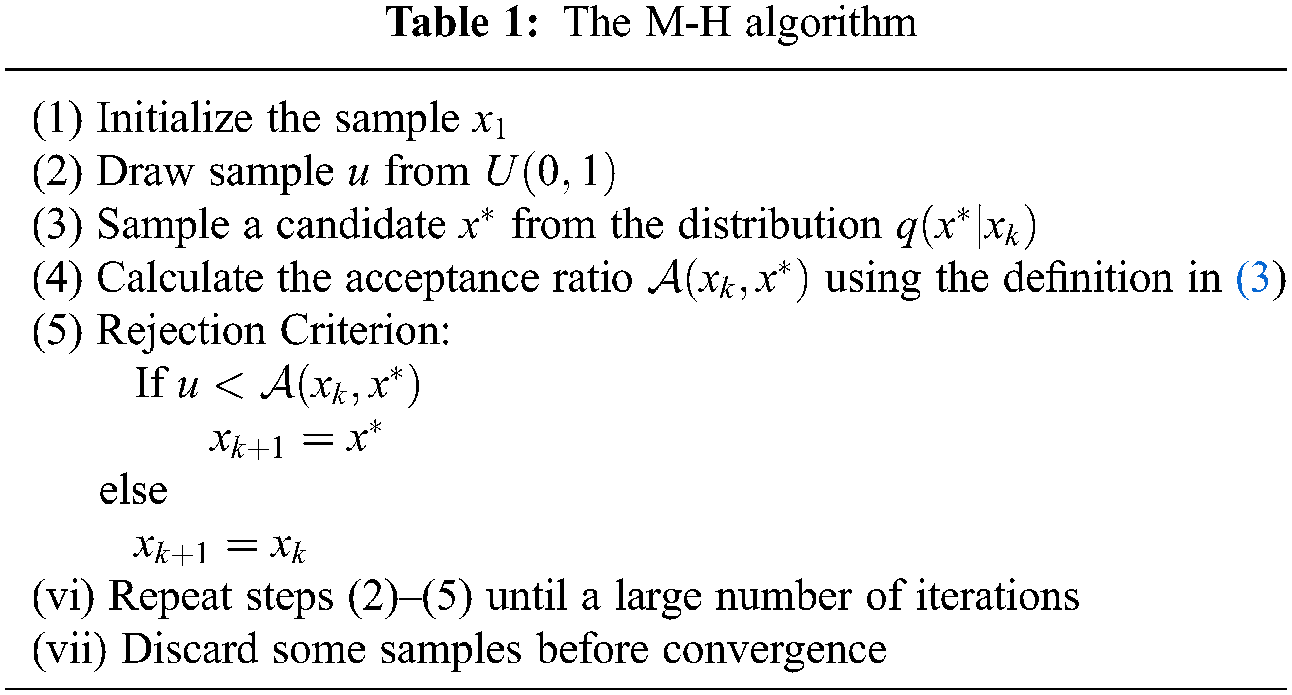
The rest of this paper is organized as follows. Section 2 reviews the main idea of the M-H algorithm. The PDF approximation of the ASαSG is shown in Section 3. In Section 4, the proposed method is then given in detail, where development of the new proposed covariance updating criterion is also provided. Computer simulations are conducted in Section 5 to verify the robust of the proposed scheme. In Section 6, conclusions are drawn.

2  The M-H Sampling Method

A Markov chain [38–41] can be defined by a series of random variables { xk }, which is

x1,x2,⋯,xk,xk+1,⋯, (1)

where xk+1 relies only on xk , and the conditional PDF is expressed as p(xk+1|xk).

Denote the PDF of xk+1 as f(xk+1) . The Markov chain is assumed to be stationary when

f(x)=limk→∞p(xk+1|xk)f(xk), (2)

is satisfied with f(x) being defined as limk→∞f(xk) . That is to say, for a stable Markov chain, with stationary PDF f(x) , the variables produced by p(xk+1|xk) will be eventually tend to be sampled from f(x) . Therefore, to obtain a proper Markov chain, the choice of p(xk+1|xk) is important and difficult in the real-world applications.

However, in some scenarios of complicated target PDF, the proper conditional PDF p(xk+1|xk) of the chain is difficult to be selected. To avoid the choose of the conditional PDF, the M-H algorithm [42,43] is developed, which is to draw samples from a proposal distribution with a constraint of a rejection criterion. Denote the sample from the proposal distribution q(x∗|xk) as x∗ , which is the candidate of the Markov chain. The rejection criterion is also required to determine whether this candidate is accepted as the member of the chain or not. The acceptance probability [28], referred to as A(xk,x∗) is utilized to describe the rejection criteria, with the definition of

A(xk,x∗)=min{1,q(xk|x∗)f(x∗)q(x∗|xk)f(xk)}. (3)

Usually, the q(x∗|xk) are chosen as some simple distributions, such as uniform or/and Gaussian. Then the steps of the M-H method are described in Tab. 1.

3  The PDF Approximation of Mixture Noise

The ASαSG noise q can be modelled as:

q=e+g, (4)

where e denotes the SαS noise with unknown dispersion γ and g follows the normal distribution with unknown variance σ2 [28].

Since the mixture noise is the additive of two random variables with different PDF, the PDF of mixed noise q, is usually calculated according to the convolution of SαS and Gaussian PDFs, which is

f(q|σ2,γ)=fG(q|σ2)∗fα(q|γ)=∫−∞∞fα(q−τ;γ)fG(q|σ2)dτ, (5)

where fG(q|σ2) and fα(q|γ) denote the PDFs of Gaussian and SαS distributions, respectively.

As the SαS process has no closed-from PDF expression, it is usually expressed using characteristic function (CF) [44], which is

φ(t)=exp⁡(jδt−γ|t|α),0<α≤2 (6)

where α is the characteristic parameter [7] reflecting the impulsiveness of the distribution, δ denotes the location parameter setting to 0 in our assumption and γ is the dispersion parameter describing the diffuseness of the process. Noticed that in the case of α=2 , the process is the normal distribution with γ corresponding to the variance. While α=1 , it corresponds to the Cauchy distribution.

Due to the complicated relationship between the CF and PDF, the PDF of ASαSG in (8) cannot be expressed with an analytic form due to the convolution and integral operations. Therefore, to obtain the closed-form PDF expression, we use the approximated PDF of the SαS noise. Because for a SαS variable, α=1 corresponds to the Cauchy distribution, and α=2 is the Gaussian process, its PDF is rewritten as the sum of a Cauchy ( α=1 ) PDF and a Gaussian ( α=2 ) PDF [38]:

fα(e|γ)=ξ(α)f1(e|η)+(1−ξ(α))f2(e|λ2), (7)

where 0≤ξ(α)≤1 is the mixed coefficient, f1(e|η) and f2(e|λ) denote the unnormalized Cauchy and Gaussian processes, with the dispersion η and variance λ2 [38], respectively. For the sake of the analytical form of ξ(α) , f1(e|η) and f2(e|λ2) , previous works [45–47] are developed, among which the most accurate expression is

ξ(α)=2Γ(−p/α)−αΓ(−p/2)2αΓ(−p)−αΓ(−p/2), (8)

f1(e|γ)=γπ(e2+γ2), (9)

f2(e|γ2)=12πγexp⁡(−e24γ2), (10)

where p denotes the fractional moment. According to the investigation in [48], the value of p is usually chosen as −1/4.

Then we express the PDF of the Gaussian variable g as

fG(g|σ2)=12πσexp⁡(−gn22σ2). (11)

With the use of (10)–(14), the PDF of ASαSG distribution in (8) is simplified as

f(q|σ2,γ)=ξ(α)f3(q|γ,σ2)+(1−ξ(α))f4(q|γ2,σ2), (12)

where

f3(q|γ,σ2)=f1(q|γ)∗fG(q|σ2), (13)

f4(q|γ2,σ2)=f2(q|γ2)∗fG(q|σ2). (14)

According to [32], f3(q|γ,σ2) and f4(q|γ2,σ2) are in fact the Voigt profile and Gaussian distribution’s PDF, whose expression are

f3(q|γ,σ2)=Re{ω}σ2π, (15)

f4(q|γ2,σ2)=12π(σ2+2γ2)exp⁡(−q22σ2+4γ2), (16)

where ω=exp⁡(−(q+iγσ2)2(1+2iπ∫0q+iγexp⁡(t2)dt)) .

4  Proposed Method

In general, the observations have the form of:

yn=sn+qn, (17)

where qn denotes the independent and identically distributed (i.i.d.) ASαSG noise term, and

sn=Acos⁡(ωn+ϕ)=a1cos⁡(ωn)+a2sin⁡(ωn), (18)

with a1=Acos⁡(ϕ),a2=−Asin⁡(ϕ) . Here A, ω and φ are amplitude, frequency and phase, respectively. The task of the estimation is to find ω from observations {yn}n=1N .

4.1 Posterior of Unknown Parameters

Let θ=[a1,a2,ω,γ,σ2]T , which is the unknown parameter vector. According to [49], the priors of noise parameter γ and σ2 , are usually considered following the conjugate inverse-gamma distribution. Assuming that the priors for θ and the observed data yn are statistically independent, they can be expressed as

f(yn|θ)=fG(yn−sn|γ,σ2), (19)

f(a1,a2)=12πδexp⁡(−a12+a222δ2), (20)

f(ω)=1π,ω∈[0,π], (21)

f(γ)=β1α1Γ(α1)exp⁡(−β1γ), (22)

f(σ2)=β2α2Γ(α2)exp⁡(−β2σ2), (23)

where β1=β2=0.01 and α1=α2=10−10 according to [50].

By employing Bayes’ theorem [19], we have

f(a1,a2,ω,γ,σ2|y)=f(y|a1,a2,ω,γ,σ2)f(a1,a2)f(ω)f(γ)=CN∏n=2N{ξ(α)Re{ωn}σ2π+(1−ξ(α))exp⁡(−en22σ2+4γ2)2π(σ2+2γ2)}, (24)

where y=[y1y2⋅⋅⋅yN]T , Re{⋅} denotes the real part and

C=β1α1β2α2π2πδΓ(α1)Γ(α2)exp⁡(−β1γ−β2σ2−a12+a222δ2), (25)

ωn=exp⁡(−(en+iγσ2)2)(1+2iπ∫0en+iγσ2exp⁡(t2)dt)), (26)

with en=yn−a1cos⁡(ωn)−a2sin⁡(ωn).

Furthermore, it can be easily seen in (27) that the expectations of posteriors of the unknown parameters are their true values. Therefore, the mean of unknown parameter samples drawn by M-H algorithm are the unbiased.

4.2 Proposed M-H Algorithm

Although we have known the PDF expression of the ASαSG noise, estimators like MLE and the lp-norm methods [51], are not able to be utilized due to poor performance and convergence problems. Furthermore, since the posteriors of unknown parameters are complicated, directly sampling on them is difficult.

Therefore, in order to accurate estimate θ , the M-H algorithm is used to sample all unknown parameters. To draw samples easily, the multivariate Gaussian distribution is chosen as the M-H proposal distribution, whose PDF is

q(x|μ)=12π|∑|exp⁡(−12xT∑−1x), (27)

where x=[x1x2x3x4x5]T with all elements corresponding to the candidates of the a1,a2,ω,γ,σ2 , respectively and Σ denote covariance matrix of the proposal distribution. Since all elements in θ are assumed to be independent, Σ is a diagonal matrix, whose main diagonal entries, namely, are proposal variances. As a hyperparameter, the large value of the proposal variance makes the chain converge faster with a sharp fluctuation around the true value. On the other hand, the smaller value will cause a small-amplitude oscillation but a slower convergence rate [22]. Therefore, for a M-H algorithm, the choice of proposal variance is a difficult and meaningful task, due to its influence of the accuracy and the computational cost.

In this paper, we propose employing a batch-mode samples to update the values of the proposed variance in the proposal covariance matrix. The details of the proposal covariance matrix Σ(k) are shown in Fig. 1. With the use of the k-th estimate, denoted by θ(k) , Σ(k)(m,m) is written as

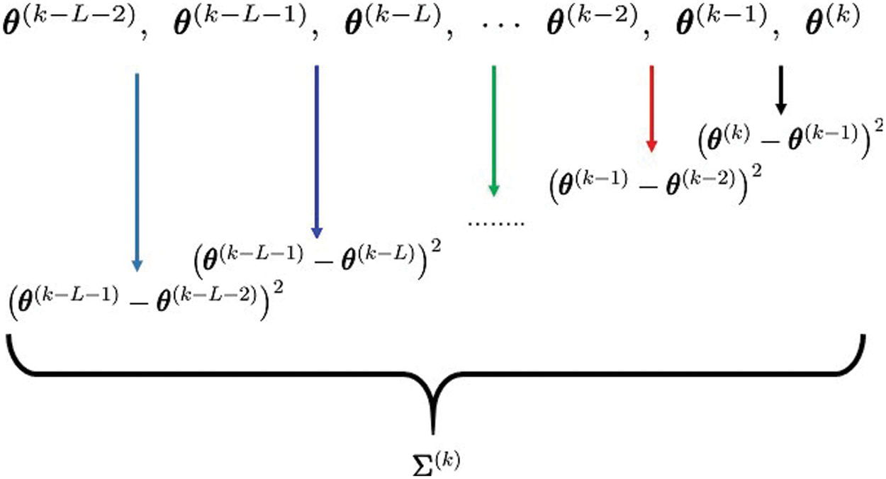
Figure 1: The batch-mode proposed covariance

Σ(k)(m,m)=∑l=0L−1(θ(k−l)−θ(k−l−1))2,m=1,⋯,5, (28)

where L is the length of the batch-mode window.

According to the previous discussion, the initialization of the M-H method, denoted by θ(1) , can be chosen arbitrarily. Then to avoid initial bias [52], we threw away the first P samples before the stable of the Markov chain, which is named the burn-in period. With the using the batch-mode proposal covariance criterion, the k-th iteration θ(k) can be obtained from the θ(k−1) using the steps in Tab. 2.

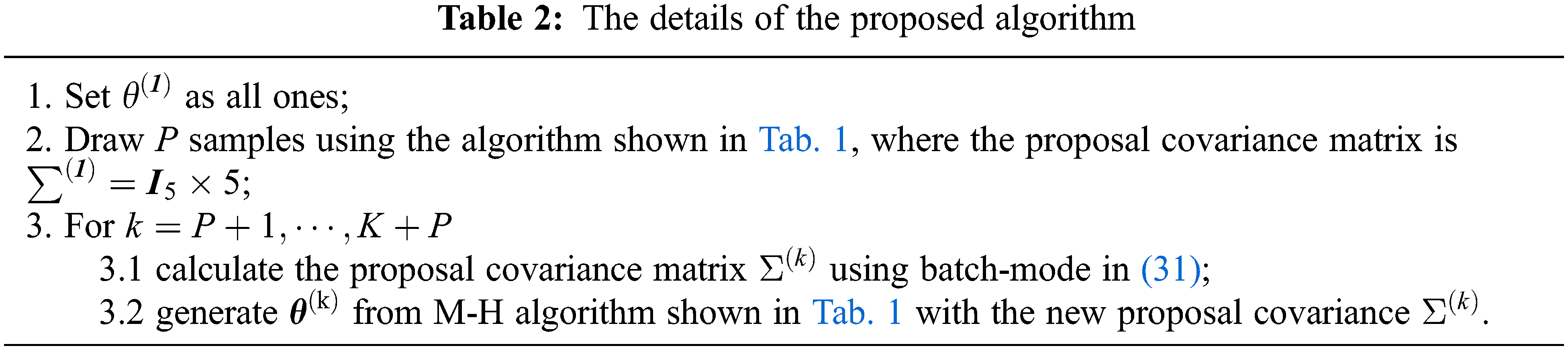
After the the steps in Tab. 2, the chain of a1,a2 and ω will be convergent and tend to their true values. Therefore, the estimates of signal parameters, referred to as a^1,a^2 and ω^ , can be obtained by the mean of θ(k)(1) , θ(k)(2) and θ(k)(3) ( k=P+1,⋯,K+P ), respectively. With the definition of a1 and a2 , the estimates of amplitude and phase, denoted by A∧ and ϕ∧ , are

A∧=a^12+a^22, (29)

ϕ∧=atan(a^2a^1), (30)

where atan(⋅) is the arctangent operator.

5  Cramér-Rao Lower Bound (CRLB)

Let ψ=[Aωϕγσ2]T. According to the definition in [22], the CRLBs of ψ can be obtained by the diagonal elements of F−1 . Here F is called the Fisher information matrix with −1 denoting the inverse operator. The (k,l) entry ( k,l=1,⋯,5 ) of F is

F(k,l)=−E{∂log⁡f(y|ψ)∂ψ(∂log⁡f(y|ψ)∂ψ)T}=−E{∑n=1N∂log⁡f(yn|ψ)∂ψ(∂log⁡f(yn|ψ)∂ψ)T}, (31)

where E{⋅} is the expectation operator and

∂log⁡f(yn|ψ)∂ψ=ξ(α)∂log⁡f3(yn|ψ)∂ψ+(1−ξ(α))∂log⁡f4(yn|ψ)∂ψ, (32)

with

∂log⁡f3(ynψ)∂ψ=1σ2Re{wn}[cos⁡(ωn+ϕ)Re{(yn−sn+iγ)wn}Ansin⁡(ωn+ϕ)Re{(yn−sn+iγ)wn}Asin⁡(ωn+ϕ)Re{(yn−sn+iγ)wn}−Re{i(yn−sn+iγ)wn}+2σ2πRe{(yn−sn+iγ)2wn}+γ2πσ2−Re{wn}2], (33)

∂log⁡f4(yn|ψ)∂ψ=f4(yn|ψ)[(yn−sn)cos⁡(ωn+ϕ)σ2+2γ2−An(yn−sn)sin⁡(ωn+ϕ)σ2+2γ2−A(yn−sn)sin⁡(ωn+ϕ)σ2+2γ2((yn−sn)2(σ2+2γ2)2−1σ2+2γ2)σ2((yn−sn)2(σ2+2γ2)2−1σ2+2γ2)γ], (34)

and sn=Acos⁡(ωn+ϕ) . According to the definition in (29), the Voigt profile is complicated. And hence, the closed-form expressions of CRLBs are not easy to be derived. Therefore, the calculation of the CRLBs in (34) adopts an approximate numerical method:

F^(k,l)≈1M∑m=1M∑n=1N∂log⁡f(ynm|ψ)∂ψ(∂log⁡f(ynm|ψ)∂ψ)T, (35)

where ynm represents the observed signal in the m-th independent trial and M denotes the number of independent runs. It can be easily to prove that (38) can approach (34) with a large M being choosing.

6  Simulation Results

In this section, computer simulations are conducted to verify the effectiveness of our method. Then the mean square frequency error (MSFE), denoted by E{(ω^−ω)2} , was employed to represent the performance measure of the estimation. The sinusoid signal sn is constructed according to (21), with all parameters being A=10.30 , ω=2.14 and φ=0.55 . While for of ASαSG noise, the shape parameter α is chosen as 1.2. The initialization of the proposed algorithm is set to all ones and the iteration number of the M-H chain is K=8000 [28]. To verify the performance, the simulations of the MLE and lp-norm estimator ( p=1.1 ) [52] are included, because they are typical robust estimators for the heavy-tailed noise. Meanwhile, the CRLB is also provided as a benchmark. In our experiments, all results are based on 600 independent runs with a data length of N=100 . Furthermore, all results are obtained by using Matlab on Intel (R) Core (TM) i7-4790 CPU@3.60GHz [22].

First of all, to obtain the proper Σ(k) in (28), the value of L is investigated. The dispersion parameters of ASαSG noise are set to γ=0.05 and σ2=0.5 [28]. Figs. 2 and 3 show the MSFE in different values of L and the computational cost vs. L, respectively. Here the computational time is measured using the stopwatch timer in the simulator. It can be seen in Fig. 2 that the MSFE of our method can be aligned with CRLB when L≥600 . While according to the result in Fig. 3, the computational cost of the proposed algorithm becomes higher for larger L. Take the higher accuracy and lower computational complexity into account, we choose L as 600 [28] in the following test.

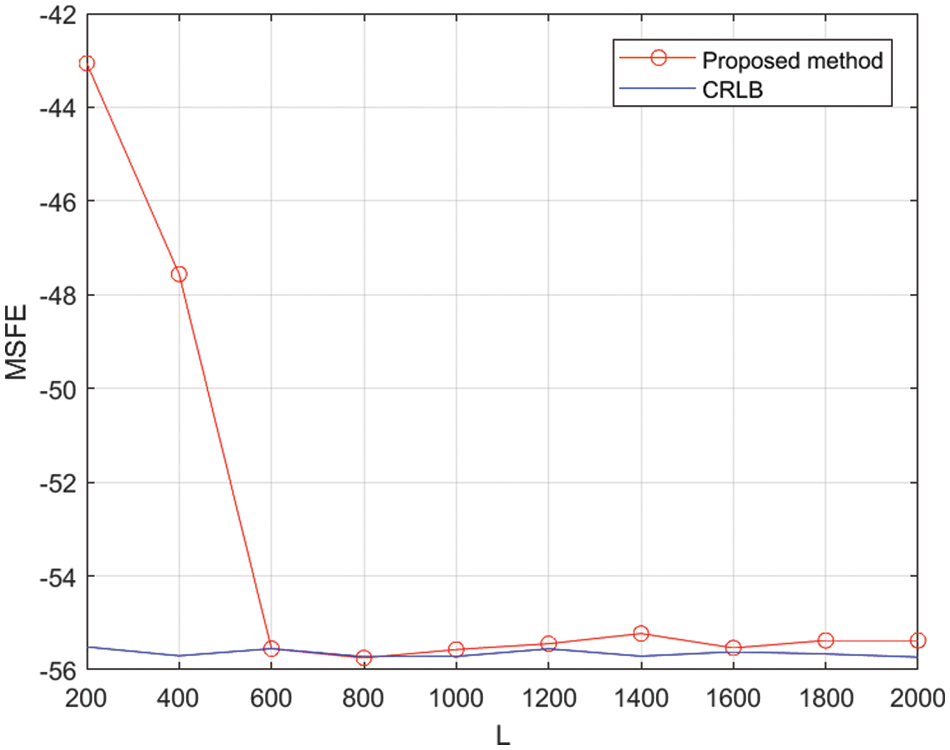
Figure 2: MSFE vs. L

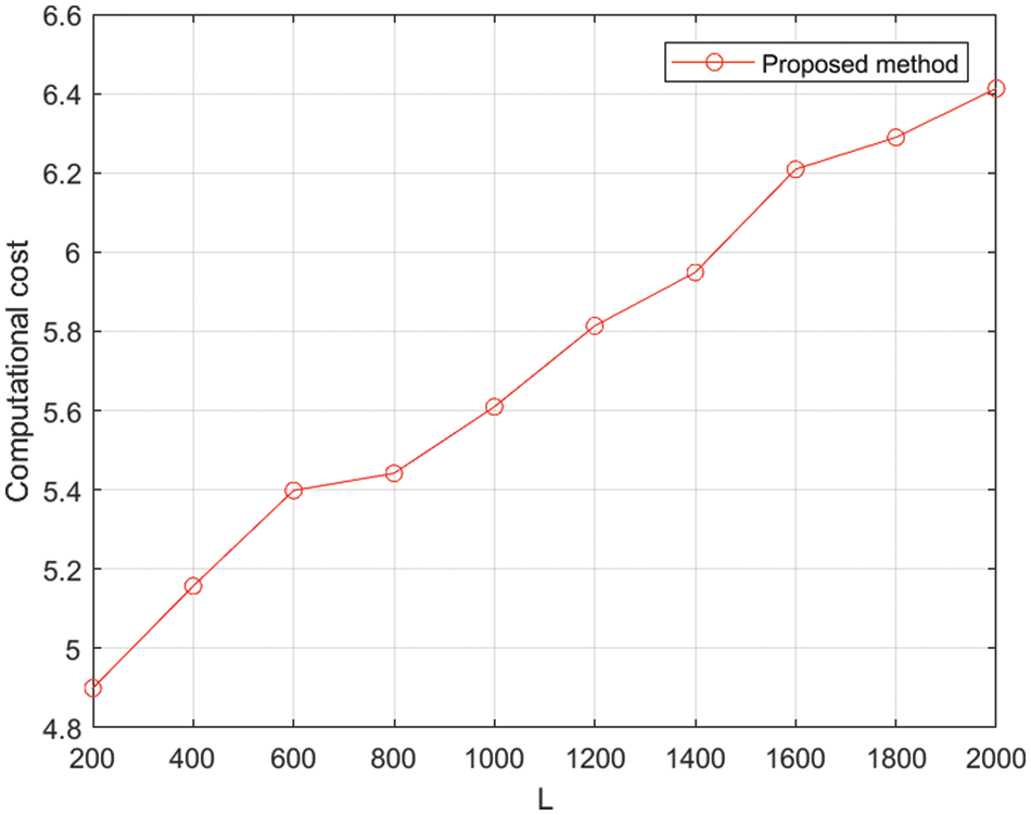
Figure 3: The computational cost of the proposed method vs. L

Second, we study the convergence rate of the M-H chain and the value of the burn-in period P. In this test, the density parameter is the same values to the previous test and the proposal covariance matrix is calculated by (31) with L=600 . Figs. 4 and 5 show the samples of ω,A,φ,γ and σ2 in different iteration k. In these figures, we can see that after the first 2000 samples, the chain of all unknown parameters approaches their true values. In this case, the corresponding burn-in period P in our simulations is 2000 [22].

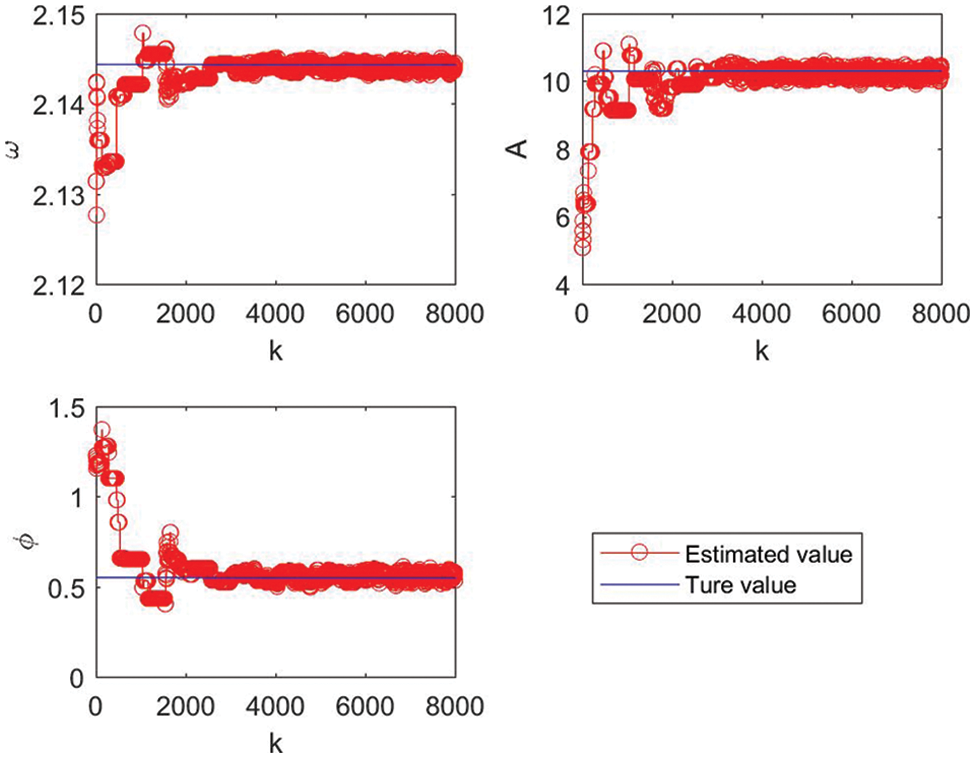
Figure 4: Estimates of unknown parameters vs. iteration number k

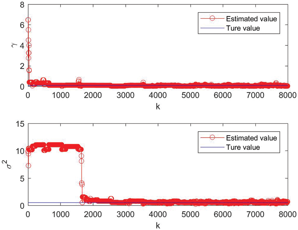
Figure 5: Estimates of density parameters vs. iteration number k

In the following, the MSFE performance of our estimator, MLE and lp-norm estimator are considered. Since there is no signal-to-noise ratio in ASαSG noise, in the proposed method, γ is scaled to generate different noise conditions. With the use of previous tests, we throw away the first 2000 samples to guarantee the stationary of the chain. It is indicated in Fig. 6 that the MSFE of our proposed method can attain the CRLB for the noise conditions γ∈[−30,5] dB [22]. Furthermore, the proposed method performs better than the lp-norm estimator and MLE, because it is much closer to CRLB.

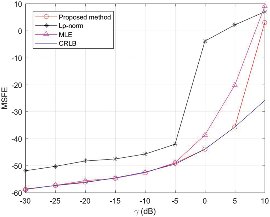
Figure 6: Mean square frequency error of ω vs. γ

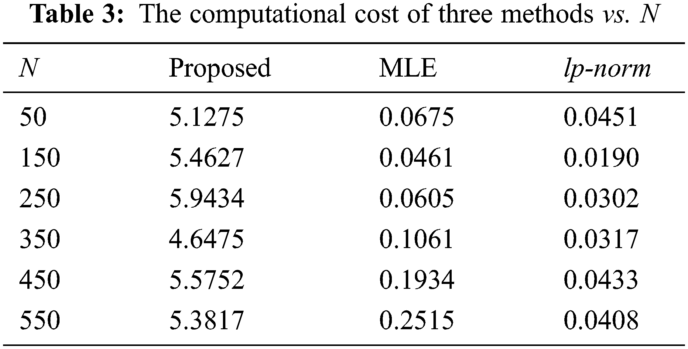
Finally, the computational complexity of our scheme is studied in different data length. It can be seen in the Tab. 3 that the computational cost of MLE and lp-norm is lower than the proposed estimator [38]. However, in the higher data length, our proposed scheme will not increase. This is to say, our method is not sensitive to the data length, indicating the advantage of its application in big data.

7  Conclusion

In this paper, the improved Bayesian method, namely M-H algorithm, is used to study the accurate frequency estimation method of single sinusoidal signal with ASαSG noise. In order to reduce the computational cost, a new proposal covariance matrix reconstruction criterion and an PDF approximation is designed. Simulation results indicate that the developed method can obtain the unbiased estimates with a stable sampling condition. In addition, MSFE of the proposal estimator can obtain CRLB after discarding burn-in period samples. Our method can be also extended to the other complicated signal models.

Funding Statement: The work was financially supported by National Key R&D Program of China (Grant No. 2018YFF01012600), National Natural Science Foundation of China (Grant No. 61701021) and Fundamental Research Funds for the Central Universities (Grant No. FRF-TP-19-006A3).

Conflicts of Interest: The authors declare that they have no conflicts of interest to report regarding the present study.

References

1. P. H. Vincent and T. Lang, Signal Processing for Wireless Communication Systems. The Netherlands: Kluwer Academic, 2002. [Google Scholar]
2. M. Bhoopathi and P. Palanivel, “Estimation of locational marginal pricing using hybrid optimization algorithms,” Intelligent Automation & Soft Computing, vol. 31, no. 1, pp. 143–159, 2022. [Google Scholar]
3. K. Mal, I. H. Kalwar, K. Shaikh, T. D. Memon, B. S. Chowdhry et al., “A new estimation of nonlinear contact forces of railway vehicle,” Intelligent Automation & Soft Computing, vol. 28, no. 3, pp. 823–841, 2021. [Google Scholar]
4. S. M. Kay, Fundamentals of Statistical Signal Processing: Estimation Theory. Prentice-Hall, NJ: Englewood Cliffs, 1993. [Google Scholar]
5. A. M. Zoubir, V. Koivunen, Y. Chakhchoukh and M. Muma, “Robust estimation in signal processing: A tutorial-style treatment of fundamental concepts,” IEEE Signal Processing Magazine, vol. 29, no. 4, pp. 61–80, 2012. [Google Scholar]
6. R. C. Gonzalez and R. E. Woods, Digital Image Processing. New Jersey: Pearson Prentice Hall, 2008. [Google Scholar]
7. Y. Chen, E. E. Kuruoglu and H. C. So, “Estimation under additive Cauchy-Gaussian noise using Markov chain Monte Carlo,” in Proc. of IEEE Workshop on Statistical Signal Processing (SSP 14), Gold Coast, Australia, pp. 356–359, 2014. [Google Scholar]
8. C. L. Nikias and M. Shao, Signal Processing with Alpha-Stable Distribution and Applications. New York: John Wiley & Sons Inc, 1995. [Google Scholar]
9. J. F. Zhang, T. S. Qiu, P. Wang and S. Y. Luan, “A novel cauchy score function based DOA estimation method under alpha-stable noise environments,” Signal Processing, vol. 138, no. 17, pp. 98–105, 2017. [Google Scholar]
10. K. Aas, “The generalized hyperbolic skew student’s t-distribution,” Journal of Financial Econometrics, vol. 4, no. 2, pp. 275–309, 2006. [Google Scholar]
11. B. Jorgensen, Statistical Properties of the Generalized Inverse Gaussian Distribution. Heidelberg, Germany: Springer-Verlag, 1982. [Google Scholar]
12. T. Zhang, A. Wiesel and M. S. Greco, “Multivariate generalized Gaussian distribution: Convexity and graphical models,” IEEE Transactions on Signal Processing, vol. 61, no. 16, pp. 4141–4148, 2013. [Google Scholar]
13. J. J. Shynk, Probability, Random Variables, and Random Processes: Theory and Signal Processing Applications. Hoboken, N.J: Wiley, 2013. [Google Scholar]
14. T. Poggio and K. K. Sung, Finding Human Faces with a Gaussian Mixture Distribution-based Face Model. Berlin Heidelberg, Germany: Springer, 1995. [Google Scholar]
15. J. T. Flam, S. Chatterjee, K. Kansanen and T. Ekman, “On mmse estimation: A linear model under Gaussian mixture statistics,” IEEE Transactions on Signal Processing, vol. 60, no. 7, pp. 3840–3845, 2012. [Google Scholar]
16. J. Zhang, N. Zhao, M. Liu, Y. Chen and F. R. Yu, “Modified Cramér-Rao bound for M-FSK signal parameter estimation in Cauchy and Gaussian noise,” IEEE Transactions on Vehicular Technology, vol. 68, no. 10, pp. 10283–10288, 2019. [Google Scholar]
17. C. Gong, X. Yang, W. Huangfu and Q. Lu, “A mixture model parameters estimation algorithm for inter-contact times in internet of vehicles,” Computers, Materials & Continua, vol. 69, no. 2, pp. 2445–2457, 2021. [Google Scholar]
18. J. N. Hwang, S. R. Lay and A. Lippman, “Nonparametric multivariate density estimation: A comparative study,” IEEE Transactions on Signal Processing, vol. 42, no. 10, pp. 2795–2810, 1994. [Google Scholar]
19. D. Herranz, E. E. Kuruoglu and L. Toffolatti, “An α-stable approach to the study of the P(D) distribution of unresolved point sources in CMB sky maps,” Astronomy and Astrophysics, vol. 424, no. 3, pp. 1081–1096, 2004. [Google Scholar]
20. J. Ilow, D. Hatzinakos and A. N. Venetsanopoulos, “Performance of FH SS radio networks with interference modeled as a mixture of Gaussian and alpha-stable noise,” IEEE Transactions on Communications, vol. 46, no. 4, pp. 509–520, 1998. [Google Scholar]
21. D. S. Gonzalez, E. E. Kuruoglu and D. P. Ruiz, “Finite mixture of α-stable distributions,” Digital Signal Processing, vol. 19, no. 2, pp. 250–264, 2009. [Google Scholar]
22. X. L. Yuan, W. Bao and N. H. Tran, “Quality, reliability, security and robustness in heterogeneous systems,” in 17th EAI International Conf., QShine 2021, Virtual Event, Springer, 2021. [Google Scholar]
23. G. Kail, S. P. Chepuri and G. Leus, “Robust censoring using metropolis-hastings sampling,” IEEE Journal of Selected Topics in Signal Processing, vol. 10, no. 2, pp. 270–283, 2016. [Google Scholar]
24. W. Aydi and F. S. Alduais, “Estimating weibull parameters using least squares and multilayer perceptron vs. bayes estimation,” Computers, Materials & Continua, vol. 71, no. 2, pp. 4033–4050, 2022. [Google Scholar]
25. M. Zichuan, S. Hussain, Z. Ahmad, O. Kharazmi and Z. Almaspoor, “A new generalized weibull model: Classical and bayesian estimation,” Computer Systems Science and Engineering, vol. 38, no. 1, pp. 79–92, 2021. [Google Scholar]
26. C. Siddhartha and G. Edward, “Understanding the metropolis-hastings algorithm,” The American Statistician, vol. 49, no. 4, pp. 327–335, 1995. [Google Scholar]
27. K. M. Zuev and L. S. Katafygiotis, “Modified metropolis-hastings algorithm with delayed rejection,” Probabilistic Engineering Mechanics, vol. 26, no. 3, pp. 405–412, 2011. [Google Scholar]
28. Y. Chen, Y. L. Tian, D. F. Zhang, L. T. Huang and J. G. Xu, “Robust frequency estimation under additive mixture noise,” Computers, Materials & Continua, vol. 72, no. 1, pp. 1671–1684, 2022. [Google Scholar]
29. C. M. Grinstead and J. L. Snell, Introduction to Probability. Rhode Island: American Mathematical Society, 2012. [Google Scholar]
30. G. James, D. Witten, T. Hastie and R. Tibshirani, An Introduction to Statistical Learning. New York: Springer, 2013. [Google Scholar]
31. X. Li, C. Peng, L. Fan and F. Gao, “Normalisation-based receiver using bcgm approximation for α-stable noise channels,” Electronics Letters, vol. 49, no. 15, pp. 965–967, 2013. [Google Scholar]
32. Y. Chen and J. Chen, “Novel SαS PDF approximations and their applications in wireless signal detection,” IEEE Transactions on Wireless Communications, vol. 14, no. 2, pp. 1080–1091, 2015. [Google Scholar]
33. X. T. Li, J. Sun, L. W. Jin and M. Liu, “Bi-parameter CGM model for approximation of α-stable PDF,” Electronics Letters, vol. 44, no. 18, pp. 1096–1097, 2008. [Google Scholar]
34. Z. Hashemifard and H. Amindavar, “PDF approximations to estimation and detection in time-correlated alpha-stable channels,” Signal Processing, vol. 133, no. 10, pp. 97–106, 2017. [Google Scholar]
35. F. W. J. Olver, D. M. Lozier and R. F. Boisvert, NIST Handbook of Mathematical Functions. Cambridge: Cambridge University Press, 2010. [Google Scholar]
36. I. S. Gradshteyn and I. M. Ryzhik, Table of Integrals, Series, and Products. Salt Lake City: Academic Press, 2007. [Google Scholar]
37. Y. Chen, E. E. Kuruoglu, H. C. So, L. -T. Huang and W.-Q. Wang, “Density parameter estimation for additive Cauchy-Gaussian mixture,” in Proc. of IEEE Workshop on Statistical Signal Processing (SSP 14), Gold Coast, Australia, pp. 205–208, 2014. [Google Scholar]
38. Y. Chen, E. E. Kuruoglu and H. C. So, “Optimum linear regression in additive Cauchy-Gaussian noise,” Signal Processing, vol. 106, no. July (4), pp. 312–318, 2015. [Google Scholar]
39. J. C. Spall, “Estimation via Markov chain Monte Carlo,” IEEE Control Systems, vol. 23, no. 2, pp. 34–45, 2003. [Google Scholar]
40. C. Andrieu, N. D. Freitas, A. Doucet and M. I. Jordan, “An introduction to MCMC for machine learning,” Machine Learning, vol. 50, no. 1/2, pp. 5–43, 2003. [Google Scholar]
41. C. Robert and G. Casella, Introducing Monte Carlo methods with R. New York: Springer Verlag, 2009. [Google Scholar]
42. S. Chib and E. Greenberg, “Understanding the metropolis-hastings algorithm,” The American Statistician, vol. 49, no. 4, pp. 327–335, 1995. [Google Scholar]
43. P. S. R. Diniz, J. A. K. Suykens, R. Chellappa and S. Theodoridis, Academic Press Library in Signal Processing: Signal Processing Theory and Machine Learning, vol. 1. New York: Academic Press, 2013. [Google Scholar]
44. E. E. Kuruoglu, “Density parameter estimation of skewed α-stable distributions,” IEEE Transactions on Signal Processing, vol. 49, no. 10, pp. 2192–2201, 2001. [Google Scholar]
45. J. F. Kielkopf, “New approximation to the Voigt function with applications to spectral-line profile analysis,” Journal of the Optical Society of America B, vol. 63, no. 8, pp. 987–995, 1973. [Google Scholar]
46. Y. Y. Liu, J. L. Lin, G. M. Huang, Y. Q. Guo and C. X. Duan, “Simple empirical analytical approximation to the Voigt profile,” Journal of the Optical Society of America B, vol. 18, no. 5, pp. 666–672, 2001. [Google Scholar]
47. H. O. Dirocco and A. Cruzado, “The Voigt profile as a sum of a Gaussian and a Lorentzian functions, when the weight coefficient depends on the widths ratio and the independent variable,” Acta Physica Polonica A, vol. 122, no. 4, pp. 670–673, 2012. [Google Scholar]
48. H. O. Dirocco and A. Cruzado, “The Voigt profile as a sum of a Gaussian and a Lorentzian functions, when the weight coefficient depends only on the widths ratio,” Acta Physica Polonica A, vol. 122, no. 4, pp. 666–669, 2012. [Google Scholar]
49. X. T. Li, J. Sun, L. W. Jin and M. Liu, “Bi-parameter CGM model for approximation of α-stable PDF,” Electronics Letters, vol. 44, pp. 1096–1097, 2008. [Google Scholar]
50. R. Kohn, M. Smith and D. Chan, “Nonparametric regression using linear combinations of basis functions,” Statistics and Computing, vol. 11, no. 4, pp. 313–322, 2001. [Google Scholar]
51. T. H. Li, “A nonlinear method for robust spectral analysis,” IEEE Transactions on Signal Processing, vol. 58, no. 5, pp. 2466–2474, 2010. [Google Scholar]
52. Y. Chen, H. C. So, E. E. Kuruoglu and X. L. Yang, “Variance analysis of unbiased complex-valued lp-norm minimizer,” Signal Processing, vol. 135, pp. 17–25, 2017. [Google Scholar]
Cite This Article
Copyright © 2023 The Author(s). Published by Tech Science Press.
This work is licensed under a Creative Commons Attribution 4.0 International License , which permits unrestricted use, distribution, and reproduction in any medium, provided the original work is properly cited.
Downloads
Citation Tools