A Novel Approach to Design Distribution Preserving Framework for Big Data

1  Introduction

Big Data (BD) is a massive collection of data [1], which is being used in a variety of application domains such as financial trading, business, education, medical, and so on [2]. Big Data is also referred to as “big data analytics.” This BD is extremely beneficial to both individuals and businesses; nevertheless, the exploitation of this BD is a difficult task since the investigation, evaluation, and data retrieval are quite complex, require a large amount of memory, and are time-consuming [3,4]. Furthermore, the data size is large, and the data structure is intricate; as a result, a larger calculation cost is required for the implementation of BD [5]. For an effective BD Analysis (BDA), the following steps must be completed: pre-processing, data structuring, partitioning phase, and data preservation phase [6–8]. In the first place, by applying the map-reduce function, the data are processed in the pre-processing phase, which reduces repetition by a factor of seven [7]. Following that, the data that was missing from the dataset is substituted or ignored [8] depending on the circumstances. Following that, the data is transformed into a normalised format. Following that, in order to improve the performance, the dimensionalities of the data are reduced [9]. Reference [10] After then, the pre-processed data is transformed into a structured format. Then, during the partitioning step, the data that is being structured is partitioned and grouped into clusters in addition to being categorised. Once this phase is completed, the clusters are sent into the classification phase, where they are processed by the classifier, allowing the user to have immediate access to the data [11,12]. Despite this, a greater correlation error is observed in BD [13], which can be attributed to the unstructured data supplied. Many techniques, such Naive Bayes [14], Gaussian Discriminant Analysis [15], and others, are proposed to address the aforementioned concerns. Other neural networks are also proposed to overcome the aforementioned issues. Despite the fact that these approaches lessen the likelihood of such issues occurring, they have some disadvantages [16]. And the drawbacks are that it is not capable of resolving aberrant situations in BD Exploration (BDE) [17], and that in order to acquire the best classification outcomes, a large number of essential criteria must be considered [18]. Certain commonly used classification approaches are not appropriate for huge datasets because, when the target classes overlap, the performance of the technique is poor [19]. The learning approaches do not address the BD issues, particularly when the material is presented in a sequential manner [20,21].

1.1 Contribution of the Research Work

A distribution preserving framework for BD is proposed utilizing the MD-PAM along with CG–ANN to conquer such difficulties. The paper’s remaining part is structure as: the related works regarding the proposed methodology are surveyed in Section 2; the proposed model of distribution Preserving Framework for BD using MD-PAM and CG–ANN is explicated in Section 3; the results together with discussion is demonstrated in Section 4. Lastly, the paper is winded up with future scope in Section 5.

2  Literature Survey

Michele Ianni and colleagues [21] pioneered the application of BDE approach. It was through this system, which operated in an unsupervised manner, that higher-quality data clusters, which were clustered around their centroids, were made available to users. The results revealed that the performance of the proposed methodology outperformed the other techniques in terms of increased accuracy and scalability, respectively. However, when the dataset had a significant amount of noise, the performance would suffer. Hernandeza et al. [22] introduced a hybrid neural architecture that combined morphological neurons with perceptrons in an integrated fashion. There were several other types of neural networks before the Morphological-Linear Neural Network (MLNN), which was the first architecture to integrate an output layer of classical perceptrons coupled with a hidden layer of morphological neurons.

Banchhor et al. [23] developed an approach for BD classification that is based on the Correlative Naive Bayes classifier and the Map Reduce Model, with the Cuckoo–Grey wolf classifier serving as the basis for the methodology (CGCNBMRM). The Cuckoo–Grey Wolf-based Optimization (CGWO) was designed through the effective incorporation of the Cuckoo Search (CS) Algorithm into the Grey Wolf Optimizer (GWO); in addition, the optimal selection of model parameters optimised the CNB model. The experience outcome shown that the approach attained accuracy, sensitivity, and specificity of 80.7 percent, 84.5 percent, and 76.9 percent, respectively, using this approach. BDE regarding data relevance was made easier by Ada Bagozi and colleagues [24], who built an IDEA as a Service (Interactive Data Exploration As-a-Service) to aid in the BDE process. In this scheme, various methodologies had been presented, including: (a) an incremental clustering approach, which provided a summarised representation of the amassed data streams; (b) for BDE, a multi-dimensional organisation of summarised data regarding various analysis dimensions; and (c) data relevance analysis methodologies, which concentrated on relevant data at the time of BDE. The MOANOFS (Multi-Objective Automated Negotiation centred Online Feature Selection) system, developed by Fatma BenSaid and colleagues [25], investigated the current enhancements of online machine learning methodologies in conjunction with a conflict resolution scheme for the improvement of classification performance in ultra-higher dimensional databases. Selcuk Aslan and colleagues [26] developed an improved Artificial Bee Colony (ABC) method that took into account the characteristics of BD optimization issues, as well as a variant known as genetic BD ABC.

2.1 Identified Drawbacks from Existing Systems

The outcomes displayed that a better outcome was attained by the scheme than the other BD optimization methodologies. Nevertheless, a poor accuracy rate was achieved by the system over the unstructured data. The existing systems consumes more time was consumed to process data; in addition, it wasn’t sensitive towards attacked data. The system was not efficient towards the correlation errors.

3  Proposed Methodology

The structured and unstructured forms data are included in the BD, which is a collection of a massive amount of data [27]. Consequently, it is a complicated task for the user to retrieve along with to recognize the appropriate data as of the larger amount of data [28]. Thus, to design the distribution preserving framework for BD, a methodology has been proposed utilizing MD-PAM and CG–ANN. Firstly, from the NSL-KDD dataset, the data are amassed and are given to the pre-processing step. In the pre-processing step, to enhance the clustering performance, the data is processed by mitigating data redundancy, dealing with the missing data, converting the data into a machine-understandable format, along with minimizing the data’s dimensionalities by employing GK–FDA. Next, the data being processed is transmuted into a structured format, which is then inputted to the partitioning phase. In the partitioning phase, by utilizing the MD-PAM, the cluster formation is performed; thus, the data with minimal distance along with minimum dissimilarities is placed in a single cluster. After that, the preserving phase is executed following the completion of data clustering. In this, the clustered data is classified by giving to the CG–ANN classifier. Thus, the data desired by the users is offered by the classification process over a big transactional database in an effortless way. Fig. 1 exhibits the proposed methodology’s architecture.

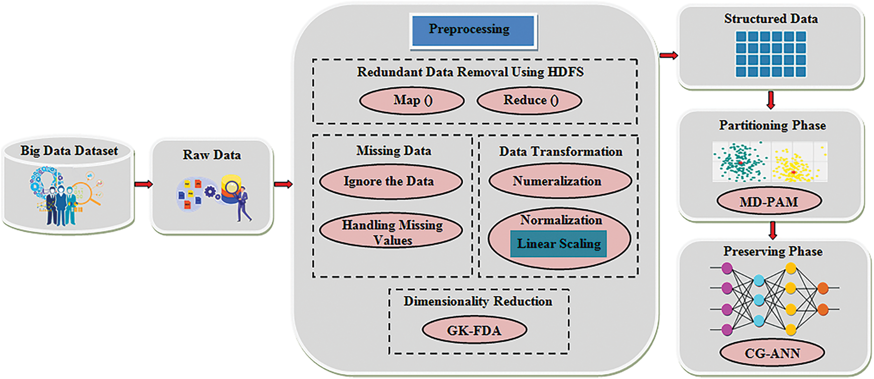
Figure 1: The architecture of the proposed work

3.1 Input Source

In the proposed system, the openly accessible NSL-KDD dataset is utilized as the input source. A massive amount of data is included in the NSL-KDD dataset, which is a classified dataset. The data values of the attacked along with non-attacked data are contained in it. Here, 80% and 20% of data are provided for the training and testing phase, respectively.

3.2 Preprocessing

In this phase, the original input data is transmuted into a supportive along with effectual format. (i) Redundant Data Removal utilizing Hadoop Distributed File System (HDFS), (ii) Missing data (iii) Data Transformation, and (iv) Dimensionality Reduction are the ‘4’ steps included in this phase. The pre-processing function is given as,

ℑ=ℑp{xdt} (1)

where, the pre-processing function’s output is specified as ℑ , the input data is signified as χdt and the pre-processing function is denoted as ℑp , which is formulated as,

ℑp={ℑrd,ℑmd,ℑdt,ℑdr} (2)

where, the redundant data removal function is indicated as ℑrd , the missing data function is specified as ℑmd , the data transformation function is proffered as ℑdt , along with the dimensionality reduction function is denoted as ℑdr .

3.2.1 Redundant Data Removal Using HDFS

Eliminating the duplicate data together with avoiding the repetition of identical data amassed in various locations are the procedures done here. Thus, it significantly mitigated the training along with execution time. The HDFS is utilized to remove the redundant data efficiently. Map as well reduce are the ‘2’ major tasks included in the HDFS. Fig. 2 displays the map-reduce function’s general structure.

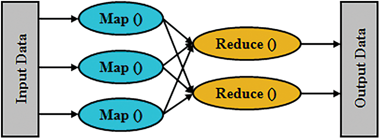
Figure 2: The general structure of the map-reduce function

(a) Map Stage

Firstly, the input data in the form of a file or directory is amassed in the HDFS. The input files are transferred to the mapper line by line. In the mapper, the input data is broken into smaller sets of data after being processed. The mapping function is given as,

ρmap(g1,δ1)=list(g2,δ2) (3)

where, ρmap specifies the mapping function, which is implemented in parallel to every pair (g1, δ1) in the dataset; in addition, creates the list of pairs (g2, δ2).

(b) Reduce Stage

The data are moved to the Reduce stage after breaking it into smaller data. The data obtained as of the mapper is processed by the reducer. A new set of outputs is produced after processing the data. These data are amassed in the HDFS. The mathematical formulation for the reduce stage is,

Rreduce(g1,list(δ2))→list((g3,δ3)) (4)

Here, the reducing function for the pair (g1,list(δ2) is signified as Rreduce and transmutes the pair into another list of ( g3,δ3) airs.

3.2.2 Missing Data

In this phase, the data is checked whether missed or not. The data being missed is substituted or rearranged. (i) Ignore the data, and (ii) Handling of missing values are the ‘2’ steps included in this phase. The missing data phase is mathematically given as,

ℑmd={h1id,h2hm} (5)

where, the missing data function is denoted as ℑmd , the ignore data function and handling missing value function are represented as h1id and h2hm, respectively.

(a) Ignore the Data

When larger numbers of data are missed or numerous values are missed then, the whole data or row is ignored. It is expressed as,

ƛ1op=h1id[xdt] (6)

where, the ignoring data function’s outcome is specified as ƛ1op .

(b) Handling Missing Values

Handling of missing values is opposite to that of the data ignoring step. Here, the missing values are substituted by random variables or average or mean regarding the missing attribute. It expressed as,

ƛ2op=h2hm[xdt] (7)

where, the outcome of handling of the missing value function is exhibited as ƛ2op .

3.2.3 Data Transformation

The procedure of transforming the data format into another needed format is termed data transformation. In this, the transformed data format is highly suitable along with machine-understandable. The ‘2’ steps included in this phase are numeralization together with normalization, which are expressed mathematically as,

ℑdt={λn,λt} (8)

where, the data transformation function is signified as ℑdt , the numeralization function is denoted as λn and the normalization function is indicated as λt.

(a) Numeralization

The string values or characters that are existed in the dataset are transmuted into a numerical format in this process. It is given as,

∅n=λn[xdt] (9)

where, the numeralization function’s outcome is specified as Øn.

(b) Normalization

In this, the data values are adjusted into a particular range betwixt 0 to 1 or −1 to 1utilizing the minimum along with a maximum of feature values to scale the data. Highly effectual access to data is provided by this approach. The data are normalized by employing Linear Scaling methodology in the proposed work. The linear scale normalization is expressed as,

λ=xtd−min(xtd)max(xtd)−min(xtd) (10)

where, the original value is indicated as χdt and the normalized value is represented as λ .To rescale the ranges betwixt the arbitrary set of values α and β , the rescaling function is formulated as,

λ=α+[xtd−min(xtd)](β−α)max(xtd)−min(xtd) (11)

where, the min-max values are signified as α and β.

3.2.4 Dimensionality Reduction

The data is converted as of a higher-dimensional space into a lower-dimensional space in the dimensionality reduction; thus, the lower-dimensional data is calculated effortlessly [29]. The GK-FDA is utilized to mitigate the data’s dimensionalities. The GK approach is hybrid to the FDA algorithm with an intention to alleviate the complications in the FDA since it is unstable under several conditions. Therefore, the reduction accuracy is enhanced considerably by the GK-FDA. Following the algorithmic steps included in GK-FDA.

Step 1: FDA is an efficient dimensionality reduction methodology that performs as maximization of various classes. In this, the data are constructed into a m×n matrix format. It is expressed as,

λ=[λ1x1λ1x2λ1xnλ2x1λ2x2λ2xnλmx1λmx2λmxn] (12)

where, mth rows specify the data, and the nth columns indicate the specific features.

Step 2: To enhance the dimensionality reduction accuracies, the input values are altered by employing GK. The mathematical formulation for GK is provided as,

f(λ)=1σ2πe−(λ−μ)22σ2 (13)

where, the input values are represented as λ , the standard deviation is specified as σ , and the mean value is signified as μ .

Step 3: The total scatter matrix δt for the mth row of the matrix with the row vector λm , is expressed as,

δt=∑n=1N⁡(λm−λmean)(λm−λmean)T (14)

where, the total mean vector is proffered as λmean.

Step 4: Λj is regarded as the set of class outcomes from the row vectors λm . It specifies the scatter δm within the matrix Λ for the class j and it is mathematically formulated as,

δm=∑λm=1N⁡(λm−λl.mean)(λm−λl.mean)T (15)

where, the mean vector for the event outcome of the class l is illustrated as λl.mean , and the transpose of matrix is illustrated as T .

Step 5: If the total number of classes is L and that are differentiated for the complete data set, the within-class scatter δw for the matrix is expressed as,

δw=∑l=1L⁡δl (16)

Step 6: The between-class scatter δb for the matrix Λ is gauged as,

δb=∑l=1L⁡nl(λl.mean−λmean)(λl.mean−λmean)T (17)

where, the between-class scatter matrix is specified as δb , the total observations within the class l is denoted as ηl .

Step 7: By considering the summation of the between-class scatter δb and within-class scatter δw for the matrix, the total scatter matrix δm is formulated as,

δm=δb+δw (18)

Step 8: The first FDA vector ϖ1 is signified as,

ω1=maxω1Tδbω1ω1Tδwω1 (19)

Step 9: The second FDA vector ϖy maximizes the scatter betwixt the L classes; however, minimizes the scatter within each class. The generalized eigen value expression’s eigenvectors ϖy is elucidated by the FDA vectors.

δbωy=elδwωy (20)

where, the extent of overall separation among the L classes is signified as el.

3.3 Structured Data

Lastly, the pre-processed data is transmuted into a structured format. The data’s reduced normalized form is mentioned as the data’s structured format. Consequently, the classification accuracy is enhanced by this structured data.

3.4 Partitioning Phase

The structured data is submitted to the partitioning phase. In this phase, regarding the data’s characteristics along with similarities, the data are partitioned and arranged into different groups or clusters [30].

Therefore, a significant impact is possessed by the classification function on the fast processing of larger data [31]. The PAM is utilized to attain the formation of the finest cluster. The PAM is nothing but a kind of K-Medoid Algorithm, which is a clustering technique pertinent to the k-means clustering algorithm. In k-medoids clustering, every single cluster is signified by one of the data points in the cluster. These points are termed cluster medoids. K-medoid is a strong alternative to k-means clustering. The K-medoid-based PAM algorithm utilized medoids as cluster centers rather than means that are used in k-means and so they are lesser sensitive to noise along with outliers than the k-means. By employing MD, the minimum distance is gauged in the PAM. Consequently, the clustering accuracy is enhanced by the MD-PAM. The Fig. 3 illustrates the pseudo-code for the MD-PAM. The following steps explicate the procedures in the cluster formation.

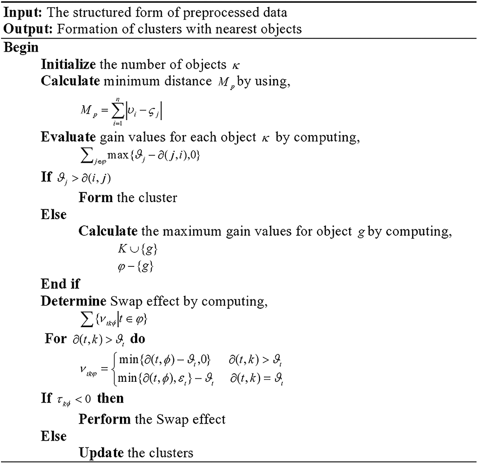
Figure 3: Pseudo-code for the MD–PAM algorithm

Step 1: Initially, by adding the number of objects with minimum distance to all other objects, the optimal medoid K is initialized. The distances betwixt the objects i and j at vi and ζj respectively are measured by the MD formula as,

Mp=∑i=1N⁡|vi−δi| (21)

Step 2: When an object i(iєA) is regarded as a candidate, then that is appended to K. After that, a total gain vi is calculated for every single object, which is given as,

γi=∑jεφ⁡max{ρj−∂(i,j),0} (22)

where, the object of Ø except I is signified as j. In case ρj > σ(I,j) then the quality of the clustering is ameliorated.

Step 3: After computing the total gain of all objects in φ , the object g that has maximum γg is chosen. It is mathematically expressed as,

K=K∪{g} (23)

φ=φ−{g} (24)

These steps are repeated until the k objects are chosen.

Step 4: The clustering quality is enhanced in the swap phase by optimizing the set of selected objects; subsequently, they are terminated by considering all swap pairs (k,ϕ)∈K∪φ and calculating the effect τkϕ on the sum of dissimilarities betwixt objects and their cluster centres by swapping k and ϕ , and then transmitting ϕ from φ to K . τkϕ is calculated as,

τkφ=∑{vtkφ|tεφ} (25)

where, the contribution of every single objects t in φ to swap k and φ is denoted as νtkϕ . If ∂(t,k)>ϑt or ∂(t,k)=ϑt , then νtkφ can be measured as.

vtkφ={min{∂(t,φ)−ρt,0);∂(t,k)>ρtmin{∂(t,φ),ϵt−ρt);∂(t,k)=ρt (26)

Step 5: To estimate whether the swapping is done or not, the pair (k,ϕ) with the minimum τkϕ is chosen. If τkϕ<0 , then, the swapping process is executed along with returned to the swap’s beginning phase. Or else, record the medoids.

Step 6: After that, the objects that are nearer to the medoids and with minimum dissimilarities betwixt the objects are grouped into the clusters, which is expressed as,

ζp={ζ1,ζ2…..ζn} (27)

3.5 Preserving Phase

The clusters formed in the partitioning phase are inputted to the preserving phase. Here, by utilizing the CG-ANN, the clustered data are classified into various classes so that the needed data can be accessed by the user effortlessly from a larger dataset. In general, owing to the need for higher memory space, higher computational complexities are faced by the ANN. Thus, to mitigate the higher memory consumption; in addition, to minimize the data’s training time, the CG is utilized in the activation function of ANN. Fig. 4 exhibits the ANN’s general structure.

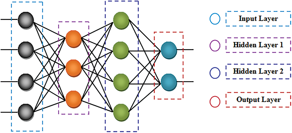
Figure 4: The general structure of the ANN

Following are the procedures included in CG-ANN.

(a) Input Layer

The input data is acquired by the input layer; subsequently, they are transmitted to the hidden layer. The input data and the respective weight values are given as,

ζi={ζ1,ζ2…..ζn} (28)

ωi={ω1,ω2…..ωn} (29)

(b) Hidden Layer

The input layer’s output is inputted to the hidden layer. In the hidden layer, input features are trained by aggregating with weight values along with bias value; subsequently, activated by the CG activation function. The classifier’s memory usage along with training time is mitigated enormously by the CG activation function, which is formulated as,

Zi=∑i=1N⁡wiτi+ba (30)

ϵh∗=Ωcg(∑i=1N⁡wiτi+ba) (31)

where, the weight values are signified as wi , the bias values that are initialized randomly are illustrated as ba , and the activation function is signified as Ωcg . Here, to activate the neurons, the CG activation function is utilized and are expressed as,

Ωcg(i+1)=k(i+1)+Ω(i)∗Δ(i);for1=0,1,2,… (32)

where, the conjugate parameter is specified as Δ(i) .

(c) Output Layer

The respective outcomes as of the classifier are delivered by the output layer. By adding all the weights of the input signal, the output unit is computed, which is expressed as,

Ψi=fs(∑ϵh∗wi+ba) (33)

where, the output unit is signified as Ψi, the hidden layers’ weights are denoted as wi, the value of the layer that precedes the output layer is defined as ξh∗ , together with the softmax function is indicated as fs. Lastly, by evaluating the target outcome with the actual outcome, the output’s loss values are calculated. Thus, the overall loss value is gauged as,

ϵrt∗=∑i=1n⁡ϵi−Ψit (34)

where, the error value is specified as ϵrt∗ , the actual outcome is signified as ξi , along with the targeted outcome is denoted as ψi . The model provides the appropriate solution if the value of the error ϵrt∗=0 ; however, the back propagation is executed by updating the weight values if the error value ϵrt∗≠0 . Lastly, the data is accessed as of the big transactional dataset effortlessly with the assist of the classification technique.

4  Result and Discussion

In this, regarding several performance metrics, the proposed framework’s final outcome is evaluated with the prevailing methodologies. The performance along with the comparative evaluation is performed to confirm the work’s efficiency. The proposed model is implemented in the working platform of JAVA and the data are acquired from the NSL-KDD dataset.

4.1 Performance Analysis of Proposed Classification Technique

The performance of the CG-ANN is evaluated with the prevailing ANN, decision tree, Naïve Bayes, along with CNN methodologies regarding performance metrics like accuracy, sensitivity, specificity, precision, recall, together with F-measure to establish the model’s efficiency.

The performance appraisal of the CG-ANN with the prevailing ANN, decision tree, naïve bayes, and CNN methodologies regarding accuracy, sensitivity, together with specificity is demonstrated in Tab. 1. The accuracy, sensitivity, and specificity attained by the CG-ANN are 97.23%, 97.34%, and 96.84%, respectively, which are ranged betwixt 96.84%–97.34%. The average rates of accuracy, sensitivity, and specificity acquired by the prevailing ANN, decision tree, naïve Bayes, and CNN methodologies are 93.58%, 93.4%, and 93.7%, correspondingly, which are comparatively lower than the proposed methodology. Thus, an accurate outcome is provided to the user by the proposed methodology.

The comparative evaluation of the CG-ANN with the prevailing ANN, decision tree, naïve bayes, and CNN methodologies regarding the accuracy, sensitivity, along with specificity is elucidated in Fig. 5. In accordance with the graphical representation, higher rates of accuracy, sensitivity, and specificity are acquired by the proposed system. However, the rates of accuracy, sensitivity, and specificity attained by the prevailing methodologies are lower than the proposed one. Therefore, the CG-ANN surpasses the existent methodologies and provides better outcomes under complicated situations.

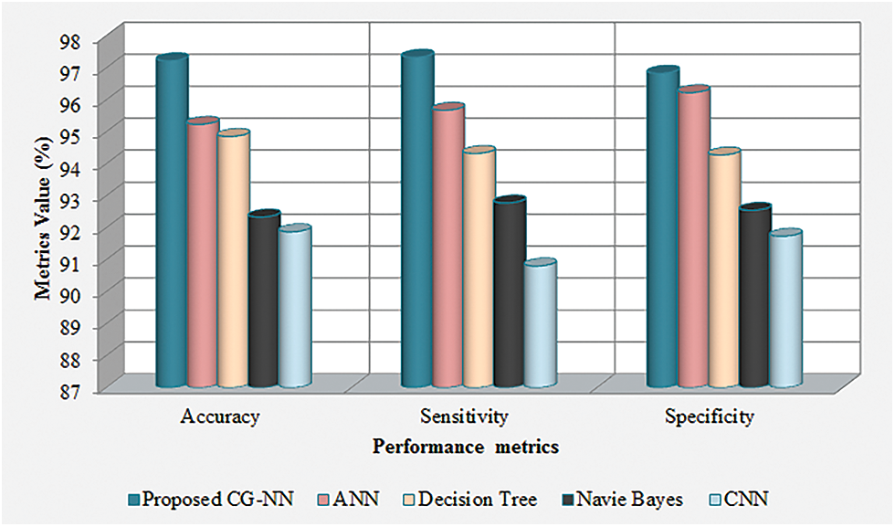
Figure 5: Graphical representation of the proposed CG-ANN based on accuracy, sensitivity, and specificity

The performance metrics like precision, recall, along with F-measure for the CG-ANN and the prevailing ANN, decision tree, naïve bayes, and CNN methodologies are illustrated in Tab. 2. The precision, recall, and F-measure obtained by the proposed model are 96.57%, 97.34%, and 96.84% whereas the prevailing ANN, decision tree, naïve bayes, and CNN methodologies acquires the precision that overall ranges betwixt 91.84%–95.26%, recall rate that overall ranges betwixt 90.81%–95.68%, and F-measure ranges betwixt 91.33%−94.68%. Thus, higher precision, recall, and F-measure values are achieved by the proposed than the prevailing models. Fig. 6 exhibits the graphical representation of Tab. 2.

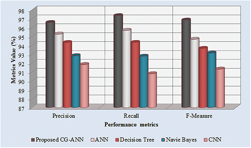
Figure 6: Graphical representation of the proposed CG-ANN based on precision, recall, and F-measure

The precision, recall, along with F-measure rates attained by the CG-ANN and the prevailing ANN, decision tree, naïve Bayes, and CNN methodologies are analogized in Fig. 6. The method should have higher precision, F-measure, together with recall rates to get better efficiency. Accordingly, the precision, recall, and F-measure attained by the CG-ANN are 96.57%, 97.34%, and 96.84%, respectively, which are higher than the prevailing methodologies. Thus, the CG-ANN alleviated the complications along with ameliorates the strength of the methodology.

4.2 Comparative Analysis of Proposed Technique in Terms of Dimensionality Reduction Time and Clustering Time

The proposed methodology’s dimensionality reduction along with clustering time is analogized with several other prevailing methodologies like Linear Discriminant Analysis (LDA), FDA, Principle Component Analysis (PCA), Singular Value Decomposition (SVD), Fuzzy C-Means (FCM), K-Means, Brich, and Mean Shift to illustrate the model’s efficiency.

The graphical assessment of the dimensionality reduction time of the GK-FDA with the existent methodologies like FDA, LDA, SVD, and PCA is demonstrated in Fig. 7. To complete the dimensionality reduction process, the time consumed by the GK-FDA is 9652 ms whereas the time utilized by the prevailing FDA, LDA, SVD, and PCA methodologies are 12354, 16874, 20145 and 24157 ms, correspondingly. Thus, it is noticed that the proposed model ameliorates the entire methodology’s running time by completing the dimensionality reduction process rapidly. Consequently, the GK-FDA’s performance is better than the prevailing methodologies.

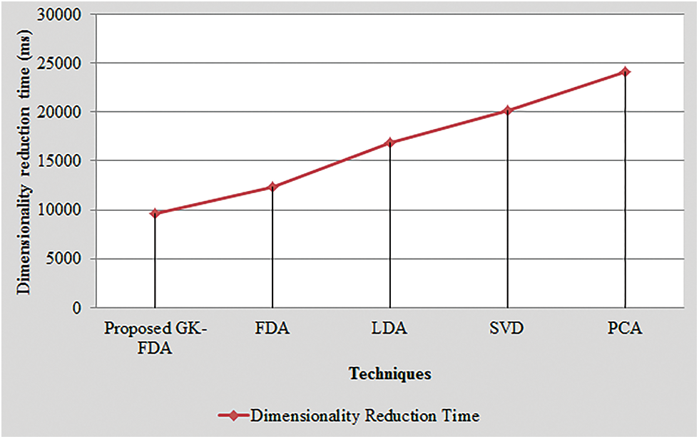
Figure 7: Graphical representation of the proposed GK-FDA based on dimensionality reduction time

The graphical view of clustering time of the MD-PAM with prevailing methodologies like FCM, K-means, Mean shift, along with Brich is depicted in Fig. 8. 17524 ms is needed by the MD-PAM to form cluster efficiently whereas the prevailing-means, FCM, Mean shift, and Brich methodologies required 22168, 26841, 30247 and 33268 ms, respectively. The existent models consume more time for cluster formation than the proposed model; thus degrading the overall system performance. Consequently, the proposed methodology consumes limited time to complete the whole process than the prevailing techniques.

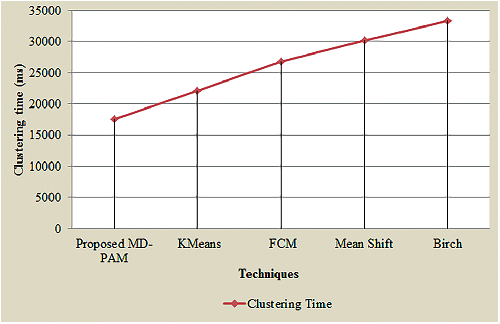
Figure 8: Graphical representation of the proposed MD-PAM based on clustering time

5  Conclusion

The proposed design the distribution preserving framework for BD, a novel technique has been proposed here utilizing MD-PAM along with CG–ANN. To certify the proposed model’s efficiency, the proposed along with the prevailing methodologies’ performance and comparative analysis are conducted regarding certain performance metrics. Several uncertainties are addressed by this methodology, which in turn provides a promising outcome. Here, the openly accessible datasets are utilized in which the accuracy, sensitivity, and specificity attained by the proposed model are 97.23%, 97.34%, and 96.84%, respectively. On the whole, the proposed methodology has better reliability along with robustness than the prevailing state-of-art methodologies. In the upcoming future, the research will be concentrated on the BD’s distribution preserving together with privacy-preserving with enhanced algorithms along with neural networks.

Funding Statement:The authors received no specific funding for this study.

Conflicts of Interest:The authors declare that they have no conflicts of interest to report regarding the present study.

References

 1.  Z. C.Dagdia, “A scalable and distributed dendritic cell algorithm for big data classification,” Swarm and Evolutionary Computation, vol. 50, pp. 1–47, 2018. [Google Scholar]

 2.  J. Ranjan and C. Foropon, “Big data analytics in building the competitive intelligence of organizations,” International Journal of Information Management, vol. 56, no. 2, pp. 1–13, 2021. [Google Scholar]

 3.  R. B. Dain, I. J. Miller, N. W. Kwiecien, D. J. Pagliarini, S. Michael et al., “Argonaut a web platform for collaborative multi omic data visualization and exploration,” Patterns, vol. 1, no. 7, pp. 1–8, 2020. [Google Scholar]

 4.  S. S. Nicolaescu, A. Florea, C. V. Kifor, U. Fiore, N. Cocan et al., “Human capital evaluation in knowledge based organizations based on big data analytics,” Future Generation Computer Systems, vol. 111, no. 4, pp. 654–667, 2020. [Google Scholar]

 5.  D. G. Rosado, J. Moreno, L. E. Snchez, A. S. Olmo, M. A. Serrano et al., “MARISMA-BiDapattern Integrated risk analysis for big data,” Computers & Security, vol. 102, no. 102255, pp. 1–25, 2020. [Google Scholar]

 6.  A. Jabbar, P. Akhtar and S. Dani, “Real time big data processing for instantaneous marketing decisions a problematization approach,” Industrial Marketing Management, vol. 90, no. 2, pp. 558–569, 2020. [Google Scholar]

 7.  A. Ekambaram, A. O. Sorensen, H. B. Berg and N. O. E. Olsson, “The role of big data and knowledge management in improving projects and project based organizations,” Procedia Computer Science, vol. 138, no. 3, pp. 851–858, 2018. [Google Scholar]

 8.  P. Lu and S. Nie, “The strength distribution and combined duration prediction of online collective actions big data analysis and BP neural networks,” Physica a Statistical Mechanics and its Applications, vol. 535, no. 3, pp. 1–16, 2019. [Google Scholar]

 9.  H. Wang, W. Wang, L. Cui, H. Sun, J. Zhao et al., “A hybrid multi objective firefly algorithm for big data optimization,” Applied Soft Computing, vol. 69, no. 1, pp. 806–815, 2017. [Google Scholar]

10. C. A. Marino and M. Marufuzzaman, “A microgrid energy management system based on chance-constrained stochastic optimization and big data analytics,” Computers & Industrial Engineering, vol. 143, pp. 1–14, 2020. [Google Scholar]

11. J. Song, Z. Ma, R. Thomas and G. Yu, “Energy efficiency optimization in big data processing platform by improving resources utilization,” Sustainable Computing Informatics and Systems, vol. 21, pp. 1–13, 2018. [Google Scholar]

12. C. B. Gonzalez, J. G. Nieto, A. J. Nebro, J. A. Cordero, J. J. Durillo et al., “JMetalSP a framework for dynamic multi objective big data optimization,” Applied Soft Computing, vol. 69, no. 4, pp. 737–748, 2017. [Google Scholar]

13. N. Krishnaraj, B. Sivakumar, R. Kuppusamy, Y. Teekaraman and A. R. Thelkar, “Design of automated deep learning based fusion model for copy-move image forgery detection,” Computational Intelligence and Neuroscience, vol. 2022, no. 8501738, pp. 1–13, 2022. [Google Scholar]

14. N. Sun, B. Sun, J. D. Lin and M. Y. C. Wu, “Lossless pruned naive bayes for big data classifications,” Big Data Research, vol. 14, pp. 27–36, 2018. [Google Scholar]

15. Y. Zhuo and Z. Ge, “Gaussian discriminative analysis aided GAN for imbalanced big data augmentation and fault classification,” Journal of Process Control, vol. 92, no. 11, pp. 271–287, 2020. [Google Scholar]

16. Y. Abdi and M. R. F. Derakhshi, “Hybrid multi objective evolutionary algorithm based on search manager framework for big data optimization problems,” Applied Soft Computing, vol. 87, no. 5, pp. 1–18, 2020. [Google Scholar]

17. N. Krishnaraj, M. Elhoseny, E. Laxmi Lydia, K. Shankar and O. ALDabbas, “An efficient radix trie-based semantic visual indexing model for large-scale image retrieval in cloud environment,” Software: Practice and Experience, vol. 51, no. 3, pp. 489–502, 2021. [Google Scholar]

18. D. Prabakaran and S. Ramachandran, “Multi-factor authentication for secured financial transactions in cloud environment,” Computers, Materials & Continua, vol. 70, no. 1, pp. 1781–1798, 2022. [Google Scholar]

19. B. Zhang, X. Wang and Z. Zheng, “The optimization for recurring queries in big data analysis system with Mapreduce,” Future Generation Computer Systems, vol. 87, no. 1, pp. 549–556, 2017. [Google Scholar]

20. A. Ahmad, M. Khan, A. Paul, S. Din, M. M. Rathore et al., “Toward modeling and optimization of features selection in big data based social Internet of Things,” Future Generation Computer Systems, vol. 82, no. 2, pp. 715–726, 2017. [Google Scholar]

21. M. Ianni, E. Masciari, G. M. Mazzeo, M. Mezzanzanica and C. Zaniolo, “Fast and effective big data exploration by clustering,” Future Generation Computer Systems, vol. 102, pp. 84–94, 2020. [Google Scholar]

22. G. Hernandez, E. Zamora, H. Sossa, G. Tellez and F. Furlan, “Hybrid neural networks for big data classification,” Neurocomputing, vol. 390, no. 1, pp. 327–340, 2019. [Google Scholar]

23. C. Banchhor and N. Srinivasu, “Integrating cuckoo search grey wolf optimization and correlative naive bayes classifier with map reduce model for big data classification,” Data & Knowledge Engineering, vol. 127, no. 11, pp. 1–14, 2020. [Google Scholar]

24. A. Bagozi, D. Bianchini, V. De Antonellis, M. Garda and A. Marini, “A relevance based approach for big data exploration,” Future Generation Computer Systems, vol. 101, no. 1, pp. 51–69, 2019. [Google Scholar]

25. F. BenSaid and A. M. Alimi, “Online feature selection system for big data classification based on multi objective automated negotiation,” Pattern Recognition, vol. 110, no. 1, pp. 1–12, 2021. [Google Scholar]

26. S. Aslan and D. Karaboga, “A genetic artificial bee colony algorithm for signal reconstruction based big data optimization,” Applied Soft Computing, vol. 88, no. 1, pp. 1–19, 2020. [Google Scholar]

27. K. S. Prakash and P. M. Joe Prathap, “Bitmap indexing a suitable approach for data warehouse design,” International Journal on Recent and Innovation Trends in Computing and Communication, vol. 3, no. 2, pp. 680–683, 2015. [Google Scholar]

28. K. S. Prakash and P. M. Joe Prathap, “Tracking pointer and look ahead matching strategy to evaluate iceberg driven query,” Journal of Computer Sciences, vol. 13, no. 3, pp. 55–67, 2017. [Google Scholar]

29. K. S. Prakash and P. M. Joe Prathap, “Efficient execution of data warehouse query using look ahead matching algorithm,” in Int. Conf. on Automatic Control and Dynamic Optimization Techniques (ICACDOT), Pune, India, pp. 9–10, 2016. [Google Scholar]

30. K. S. Prakash and P. M. Joe Prathap, “Priority and probability based model to evaluate aggregate function used in iceberg query,” International Journal of Applied Engineering Research, vol. 12, no. 17, pp. 6542–6552, 2017. [Google Scholar]

31. K. S. Prakash and P. M. Joe Prathap, “Evaluating aggregate functions of iceberg query using priority based bitmap indexing strategy,” International Journal of Electrical and Computer Engineering (IJECE), vol. 7, no. 6, pp. 3745–3752, 2017. [Google Scholar]