Intelligent Automation & Soft Computing DOI:10.32604/iasc.2023.029210
Article

Fault Diagnosis in Robot Manipulators Using SVM and KNN

D. Maincer1,*, Y. Benmahamed2, M. Mansour1, Mosleh Alharthi3 and Sherif S. M. Ghonein3

1Laboratoire de Robotiques Parallélisme et Systèmes Embarquer, Département Automatique et Control, Université des Sciences et Technologie Houari Boumediene, Algiers, Algeria
2Laboratoire de Recherche en Electrotechnique, Ecole Nationale Polytechnique, B.P 182, El-Harrach, 16200, Algiers, Algeria
3Electrical Engineering Department, College of Engineering, Taif University, P. O. Box 11099, Taif, 21944, Saudi Arabia
*Corresponding Author: D. Maincer. Email: dmaincer@usthb.dz
Received: 27 February 2022; Accepted: 14 April 2022

Abstract: In this paper, Support Vector Machine (SVM) and K-Nearest Neighbor (KNN) based methods are to be applied on fault diagnosis in a robot manipulator. A comparative study between the two classifiers in terms of successfully detecting and isolating the seven classes of sensor faults is considered in this work. For both classifiers, the torque, the position and the speed of the manipulator have been employed as the input vector. However, it is to mention that a large database is needed and used for the training and testing phases. The SVM method used in this paper is based on the Gaussian kernel with the parameters γ and the penalty margin parameter “C”, which were adjusted via the PSO algorithm to achieve a maximum accuracy diagnosis. Simulations were carried out on the model of a Selective Compliance Assembly Robot Arm (SCARA) robot manipulator, and the results showed that the Particle Swarm Optimization (PSO) increased the performance of the SVM algorithm with the 96.95% accuracy while the KNN algorithm achieved a correlation up to 94.62%. These results showed that the SVM algorithm with PSO was more precise than the KNN algorithm when was used in fault diagnosis on a robot manipulator.

Keywords: Support Vector Machine (SVM); Particle Swarm Optimization (PSO); K-Nearest Neighbor (KNN); fault diagnosis; manipulator robot (SCARA)

1  Introduction

Modern robots are highly susceptible to faults during their execution due to the highly complex nature of new-generation robotic systems and the uncertain environments they occupy [1]. However, even well-designed robotic equipment will be subject to defects during its service life. For this purpose, numerous diagnostic techniques in the literature have been investigated to solve these problems [2–6]. The detection of emerging sensor/actuator failures has been given limited attention in the literature, which is important for the operation of the robot [7]. Indeed, detecting and isolating the defect sensor/ actuator in a manipulator is not easy during the operation of the robot. Sensor measurements describe the features of the monitored system and the sensor itself. For example, any abnormal deviation in sensor readings could be caused by a change in the monitoring system.

The system is also becoming more complex as the number of interconnected sensors and subsystems increases. This increase may cause defects to appear independently or concurrently. Furthermore, the measurements can be noisy because of the imperfect nature of the sensor [7].

Therefore, isolation and defect detection estimation (FDIE) methods are important for the diagnosis of manipulation defects [2,3]. Many studies have been developed based on artificial intelligence (AI) methods such as K-Nearest Neighbor (KNN) algorithm, artificial neural networks (ANNs), linear and nonlinear regression analyses, fuzzy logic, discriminant analysis and the combination of the Sequential Floating advance quest and Fisher Projection technique [8–13]. Artificial intelligence techniques were employed to derive affective states. Then they are adapted to such diagnostic issues. In addition to the aforementioned methods, Time Delay Control (TDC), Sliding Mode Control (SMC), tolerant control of faults which are applied to contract the fault effect based on fault detection, and neural networks with TDC [14–20].

In other words, the machine learning method was used for the automatic diagnosis of failures in many industries [21,22]. In particular, SVM is a significant machine learning method widely supported in many applications [23–25]. The SVM performance is highly dependent on the selection of certain parameters (such as kernel function and the parameters of regulation), the selection of kernel function and regulation parameters are important for SVM technique [26]. Even though, v-fold cross validation is the usually used procedure to establish the SVM model [2–4]. It requires t-times training, which in its turn needs a lot of computation (which is CPU-intensive). The SVM algorithm can be hybridized with other algorithms such as the Convolutional Neural Network (CNN) [27]. The aim of the combination is to achieve an accurate diagnosis.

The aim contribution of this paper is to approve the effectiveness of the machine learning method in diagnosing faults in a manipulator arm, it would be useful to do a comparative study between PSO-SVM and KNN algorithms. Recognizing that, the manipulating arm used here has three degrees of freedom and has been affected by defects on the three successive articulations. The proposed algorithms will be capable of detecting, isolating and identifying affected articulations, depending on the x-axis, y-axis, z-axis, xy-axis, xz-axis, yz-axis and xyz-axis. SVM parameters have been selected automatically by the PSO algorithm to improve diagnosis accuracy. In decree to have a dependable model, the Cross Validation (CV) method has been used. The application of PSO-SVM and the contrastive tests reveal the efficiency and the supremacy of the suggested technique compared to the KNN algorithm.

The remainder of the paper is organized as follows. Section 2 offers an overview of the dynamic model of the robot. Section 3 presents some reminders on KNN and SVM-PSO algorithms. Section 4 specifies the simulation results and discussions. Finally, Section 5 concludes the document and provides guidance for future work.

2  Problem formulations

Manipulative robots are represented by dynamic equations that are found thanks to the Lagrangian formulation, so the equation of a manipulator is written as follows [28]:

M(q)q¨+C(qt,q˙t)q˙t+G(q)=τ (1)

where G(q) is the vector of gravitational force, C(q,q˙) is the matrix of centrifuge and Coriolis, M(q) the inertia matrix, τϵRn is the vector torque, qϵ¨⁡Rn,q˙ϵRn,qϵRn are angular acceleration, the angular velocity, and the angle of the joints, respectively [28]. In this paper, the dynamic equations of the SCARA robot have been utilized for the simulation.

The additive fault sensors signified by:

qt=q+Δq (2)

where:

•    qt is the sensor’s joint measurement;

•   q is the sensor’s joint fault-free measurement;

•    Δq is the supposed sensor fault;

Then the dynamic Eq. (3) can be obtained by replacing Eq. (2) in Eq. (1).

M(qt)q¨t+C(qt,q˙t)q˙t+G(qt)=τt (3)

Where:

•    M(qt) is the inertia matrix;

•    C(qt,q˙t) is the matrix of Coriolis and centrifuge;

•    G(qt) is the vector of gravitational force;

•    τt is the control input torque;

3  K-Nearest Neighbor (KNN)

KNN, which is a supervised learning algorithm, usually applied to signal processing, pattern recognition, image processing, medical, etc. [29]. The algorithm assumes that the closest position for acquisitions falls into the same category. The technique is developed to compute the distance between the test point and the drive samples [30]. Thus, the nearest neighbors are found from the training dataset to determine which class label is the most common. The k closest data points are studied with the aim of assigning to the data points being analyzed [31].

The value of k is chosen so that it is not too small, thus that the noise effect is minimized in the training dataset. On the other hand, when the value of k is large, this influences the increase in the computation time. This consists in choosing for an example x the class y=ωj of its closest neighbor j [31]:

DKNN(x)=ωj|j=argmin1≤i≤md(x,xi) (4)

With d(x,xi) is a metric allowing to measure the distance between two examples. To avoid being too sensitive to noisy data, we often search for the KNN. Let us denote by NN(x,k,ωi,Zm) the function returning the number of examples of the class ωi among the k nearest neighbors of x . The selected class is the one which is the majority among these k neighbors, which corresponds to the following decision function:

DkNN(x)=argmaxωi∈yNN(x,k,ωi,Zm) (5)

The pseudo code of KNN algorithm can be established as follows:

Begin

For each example(x,c)ϵA

Calculate the distance d(x′,x)

End

For each xϵKNN(x′) do

Count the number of occurrences of each class

End

Assign to x′ the most frequent class

End

4  Support Vectors Machine (SVM)

The SVMs are a pioneer machine learning tool suited for classification, prediction and regression. The purpose of using SVM is to find the optimal solution between two classes. When the number of samples is infinitely large one obtains the optimal solution. In particular, it has a good generalization even when the samples are few [32].

The SVM decision function can be written as follows:

f(x)=wx+b=∑k=1m⁡wkxk=0 (6)

where f(x) results Classifications of test data, wweight , bbiase , x Kernel test data calculation [33]. In order to satisfy the constraints, the hyperplane must be definitely separated. In other words:

f(xk)≥1 if yk=1 => xk be owned by to class 1 and

f(xk)≤−1 if yk=−1 => xk be owned to class -1

The merging of these constraints gives the following result:

yk(wxk+b)≥1fork=1,2,…,m (7)

In the case of non-linear separation of two classes, the variable ξk is introduced in Eq. (7), and it then becomes:

yk(wxk+b)≥1−ξkfork=1,2,…,m,and0<ξk (8)

The conditions below must be satisfied by the separating hyperplane:

{yk(wxk+b)≥1min12‖w‖2 (9)

Obviously, ‖w‖2=wTw , minimizing the norm makes the margin maximum.

In order to get the optimal solution of the hyperplane, the Lagrangian principle has been utilized:

L(w,b,∝)=12‖w‖2−∑k=1m⁡αk[yk(wTxk+b)−1] (10)

∝ is a set of Lagrnage coefficients (∝k)>0

By introducing the following optimal conditions

{∂L(w,b,a)∂w=0∂L(w,b,a)∂b=0 (11)

We obtain:

{w=∑k=1m∝kxkyk∑k=1m∝kxk=0 (12)

We solve the problem using the following form:

{maxL(w,b,a)w=∑k=1m∝kxkyk∑k=1m∝kxk=0∀k,∝k≥0 (13)

This is equivalent to the following equation:

{max∑k=1m∝k−12∑k,j∝k∝jykyj(xk,xj)∑k=1m∝kxk=0∀k,∝k≥0 (14)

We integrate the deviation variable k as follows:

yk(wxk+b)≥1−ξksuchask=1,2,…,m∀k,0<ξ<1 (15)

We obtain the following optimization problem:

{min12‖w‖2+C∑k=1m⁡ξkyk(wxk+b)≥1−ξksuchas∀k,0<ξk<1k=1,2,…,m (16)

where C is the margin parameter.

The lagrangian is defined as follows:

L(w,b,ξ,x)=12‖w‖2+c∑k=1m⁡ξk−∑k=1m∝k[yk(wTxk+b)−1+ξk (17)

If we apply the Karush-Kuhn-Kucker conditions which are the second order optimization conditions:

{∂L(w,b,ξ,∝)∂w=0∂L(w,b,ξ,∝)∂b=0∂L(w,b,ξ,∝)∂ε=0 (18)

We obtain:

{max∑k=1m⁡αk−12∑k,j⁡αkαjykyj∅(xk)∅(xj)suchas∀k,αk≥0∑k=1m∝kxk=0 (19)

In the SVM networks, the product ∅(xk)∅(xj) may be supplanted by the positive kernel function. In our case, the following Gaussian kernel function has been selected:

k(xk,xj)=exp⁡(−γ||x−x′||2) (20)

w and b define the position of the separating hyperplane as explained in the Fig. 1:

Figure 1: Separation of two classes: (a) Linear separation (b) Non-linear separation

4.1 SVM Parameters Optimization using PSO algorithm

The PSO algorithm has been developed by Kennedy and Eberhart [34] since 1995. The parameters (C,γ) of the SVM model have been optimized for the progression of the PSO algorithm, in order to increase the diagnostic precision. This algorithm was built after having had a long observation about a flock of birds and also a school of fish, while they are in search of their food. Every fish has its way between food and itself. This action is a social behavior, intelligence in swarms, leads all natural processes to find a shorter path to their walls [35].

The PSO algorithm ensures auto-selection of the SVM parameters which achieve the best diagnostic accuracy.

The optimization procedure of the SVM parameters through PSO technique is interpreted in different step as follows:

1. Initialization: N particles of populations are randomly generated by PSO, each particle with a position and a velocity in the d dimensional search space.

Moreover, the particles are named thus, Pi=(Pi1,Pi2,…,Pid) position and Vi=(Vi1,Vi2,…,Vid) speed, knowing that, Pi and Vi are matrices of N∗d . (C,γ) conditioning parameter for SVM variables

2. Training: The SVM model is trained using 90% of the database, for each particle

3. Testing: 10% of the database has been reserved to test the SVM model. The evaluation criteria representing the accuracy of each particle are calculated through Eq. (21).

fi=yt−yfiyt×100 (21)

Where yfi is the total number of false classified data, yt is the total number of testing data.

4. Updating: each particle updates the position and speed using the following equations:

Vid(t+1)=WVid(t)+C1r1(t)(pbestd(t)−pid(t))−C2r2(t)(gbestd(t)−pid(t) (22)

pid(t+1)=pid(t)+Vid(t+1) (23)

•    C1andC2 are acceleration coefficients;

•    Pi represents the position of the “i” particle;

•    Vi represents the velocity of the “i” particle;

•    r1 and r2 are random number in the range [0,1];

•    V is the inertia weight.

5. Stop criterion: Steps 2 to 4 are duplicated until reaching the maximum number of iterations.

6. Exploitation: The SVM optimal parameters acquired are utilized for classification.

The calculation process of SVM model can be summarized by the flowing flowchart in Fig. 2:

Figure 2: The SVM model with the calculation process [36]

5  Cross Validation

V-fold cross validation is a procedure for ranking or comparing the robustness of a classification algorithm on a set of data. The classification algorithm is randomly distributed by a bend dataset of equal size, and each fold is used to test the induced pattern of the other folds. Evaluating the mean of the precisions of v leads the cross-validation of v-fold to better performance of the classification algorithm, implying the level of averaging is supposedly to be in the fold. Knowing that each fold contains the same number of instances [37].

6  Simulations and results

A robot manipulator arm has been considered in this work with 3 degrees of freedom, called SCARA as described in Section 2. The robot manipulator parameters used in the simulations are introduced as follows, in order to diagnose the manipulator faults: the moments of inertia are I1 = 0.02, I2 = 0.03 and I3 = 0.05 (rad/s), m1 = 0.5, m2 = 0.3, m3 = 0.1 Kg, the length of the links is L = 1m and the sampling time is equal to ts=0.01s . In order to test the diagnosis of faulty joints, 7 classes have been supported on the x-axis, y-axis, z-axis, xy-axis, xz-axis, yz-axis and xyz-axis. One on the x-axis (D1), 10 additive samples faults have been applied with a 0.001 sampling step over an interval [0,0.02]. The second class (D2) on the y-axis, also 10 additive samples faults with a 0.001 have been introduced over the interval [0,0.02]. On the interval [0,0.03], the 10 additive samples faults have been injected on the z-axis and considered as the third class (D3). In the fourth class (D4), the 10 additive faults have been implanted on the xy-axis, on the x-axis over the interval [0,0.02] and along the y-axis on the interval [0,0.02]. On the interval [0,0.02] and [0,0.03] according to the x-axis and z-axis, the 10 additives faults have been inserted to create the D5 class. However, in the sixth class (D6), and in the intervals [0,0.02] and [0,0.03] interposed to the y-axis and z-axis, we apply 10 additive samples faults. The last class D7 (xyz-axis) which includes three variation intervals [0,0.02], [0,0.02] and [0,0.03], we introduce 10 additive samples faults. Thus, the output vector consists in: [D1 D2 D3 D4 D5 D6 D7]. The whole of the injected faults according to the 7 classes have been established with a database of 63000 samples.

Concerning the input vector, the composition consists of: the torque vector τ(τx,τy,τz), position vector q(qx,qy,qz) and manipulator speed vector q˙(q˙x,q˙y,q˙z) , and it will be represented by: [τxτyτyqxqyqzq˙xq˙yq˙z] . For classifiers, the cross validation method has been used.

The simulations have been carried out using the MATLAB software. The results are presented below.

6.1 KNN results

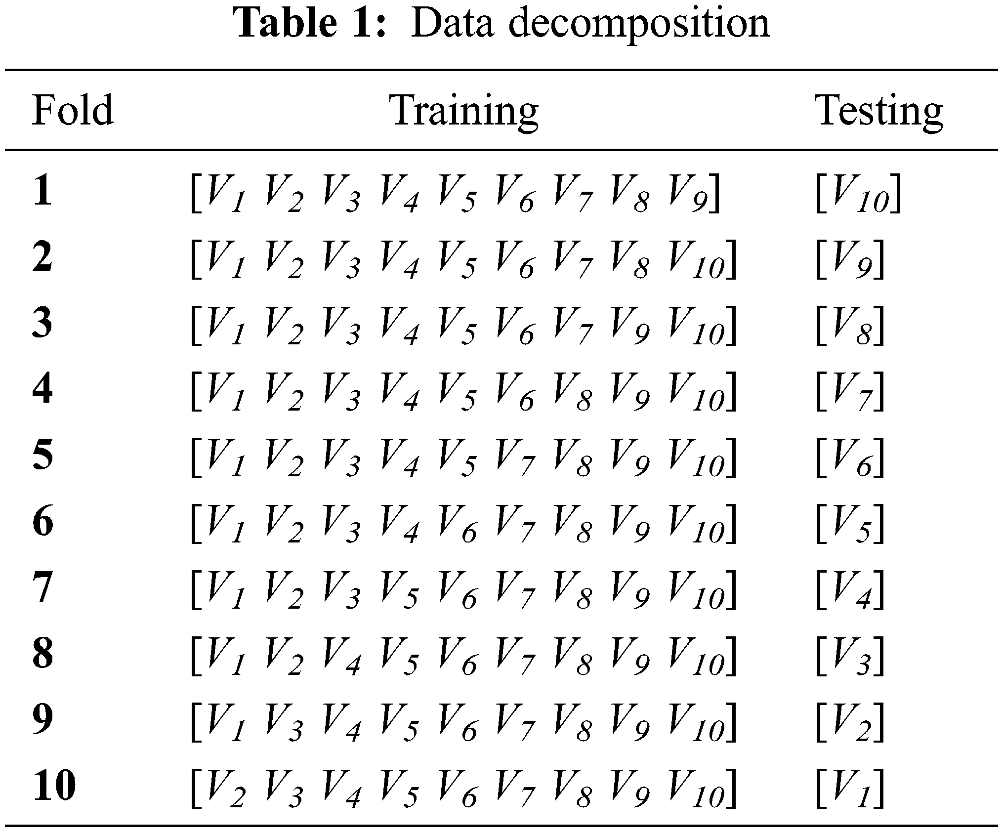
For both classifiers, the training and test procedures were initiated using the cross-validation method. 10-fold cross validations have been chosen and the database D is composed of : D = [V1 V2 V3 V4 V5 V6 V7 V8 V9 V10]. The accuracy diagnosis is assessed 10 times and the grader is assessed on the basis of the average value. Every time, for the ith test Vi is used, and the remaining of the database is reserved for the training process. Then, all accuracies rates have been evaluated on the tenth of samples population (63 000 samples) for the testing phase and on ninth of the samples population (56 700) for the training phase. Tab. 1 explains the decomposition of the data of the 10-fold cross validation method.

To obtain the highest possible diagnostic accuracy, several types of distance were used for the KNN algorithm, namely Cityblock, Cosine, Correlation and Euclidean. For the training phase, the number of neighbors k has been varied from 1 to 100 where the value corresponding to the better accuracy rate is maintained. The effect of the number of neighbors was also investigated, Fig. 3 shows clearly this influence (the first cross validation taken as example).

Figure 3: The impact of the distance type and number of neighbors on accuracy diagnosis

From the obtained results in Fig. 3 of the first fold validation, it becomes clear the extent of the effect of the number of neighbors on the diagnosis accuracy. An accuracy diagnosis of 99.69% has been obtained for correlation distance with k = 1, the cosine comes in second place with an accuracy of 99.55 and k = 1. Accuracy of 99.50% and 99.03% have been achieved for the Euclidian and city block respectively with k = 1 for both distances. The results of the 10 folds validation are summarized in Tab. 2. For each validation, it is clear the extent of the impact of distance type and neighbors value.

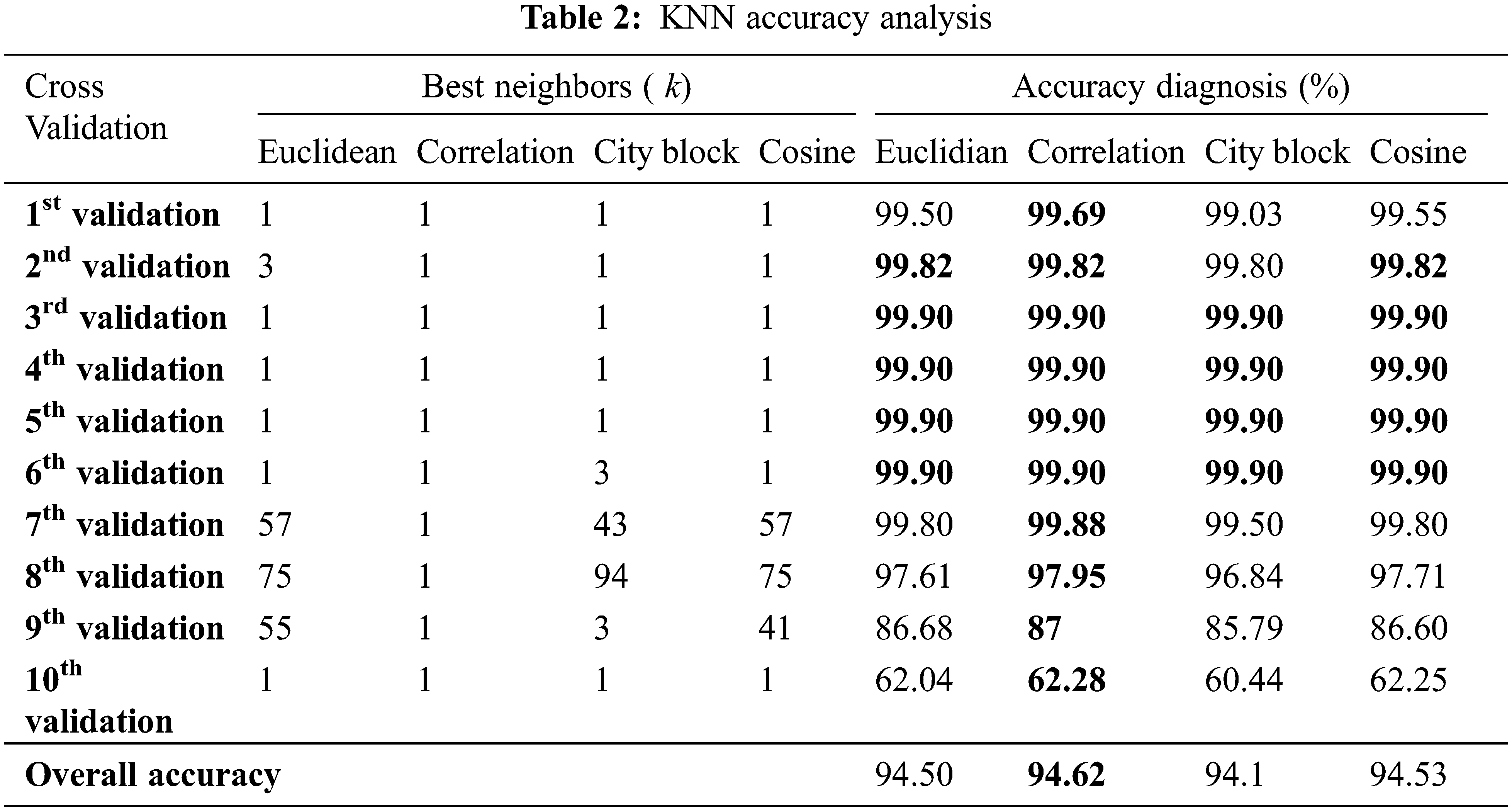
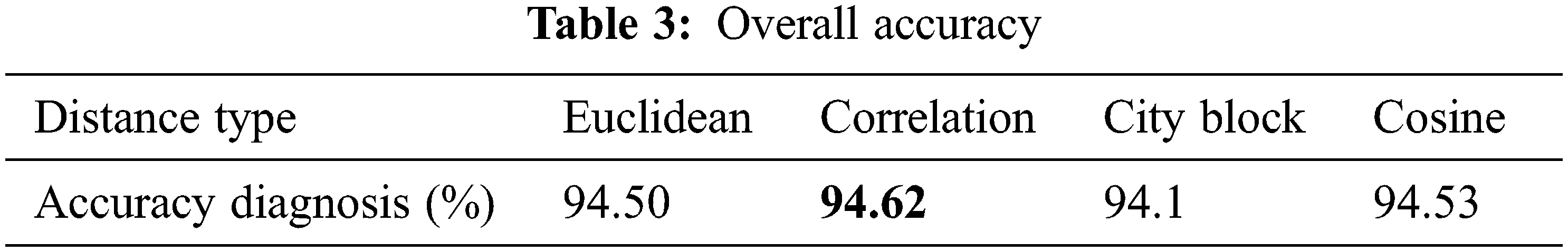
The overall accuracy of each distance type is represented in Tab. 3. The results are given for the four distance types, such as, Euclidean, Correlation, City block and cosine. It was found that the best accuracy of the KNN algorithm was 94.62% with a correlation distance type against 94.53 for cosine distance type. The Euclidean and the City block distances have achieved 94.50% and 94.10% respectively.

6.2 SVM results

The SVM parameters C and ɣ are adjusted using PSO. The results of the simulations show that the approach makes it possible not only to select important characteristics, but also to obtain high precision for the classification of faults. PSO affects the precision of the SVM after hybridization of SVM-PSO. The SVM-PSO method performs better than the SVM on the benchmark dataset of the reviewer’s dataset. Fig. 4 shows the evolution performance of the SVM classifier during optimization process using PSO algorithm for the first validation. The PSO algorithm has been employed to the auto selection of parameters (C, γ) for the gaussian kernel. Fig. 4 proves the influence of parameters values on the accuracy results.

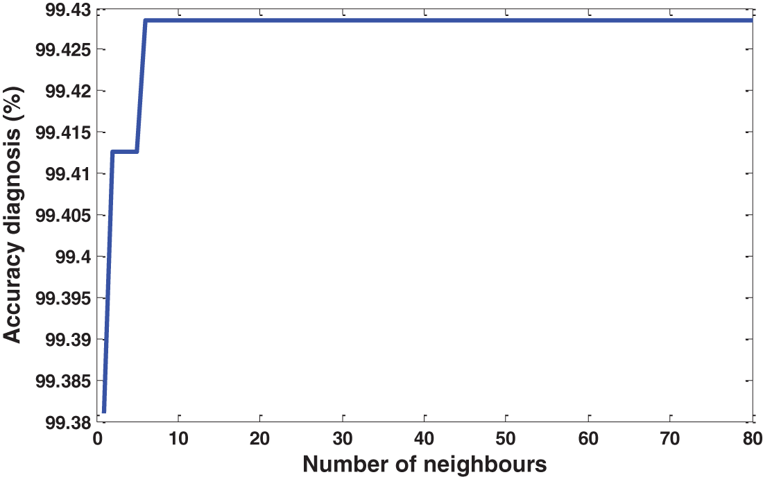
Figure 4: Performance of PSO-SVM classifiers

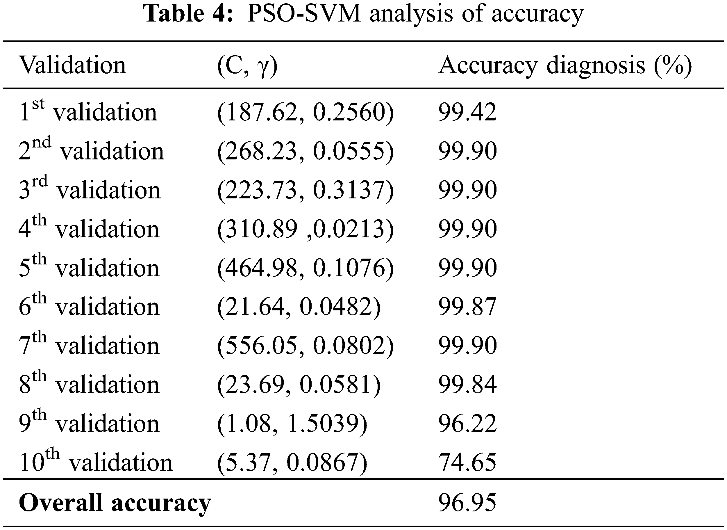
The results presented in Tab. 4 for cross-validation 10; in each cross-validation, the parameters (C, γ) that provided the highest possible accuracy are different. Subsequently, the PSO algorithm was helpful in adjusting the C and γ parameters.

Tab. 5 presents the dataset used in the simulations. In fact, has been finding 7 classes of faults in which the value of the fault for each input is given.

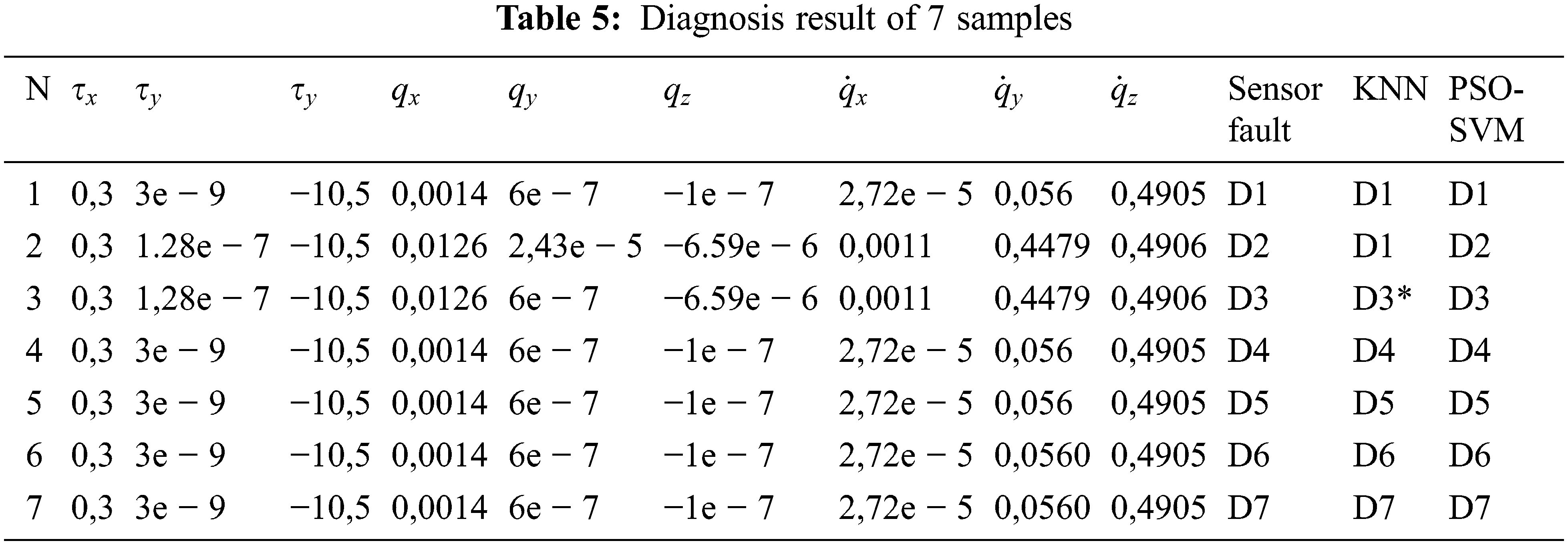
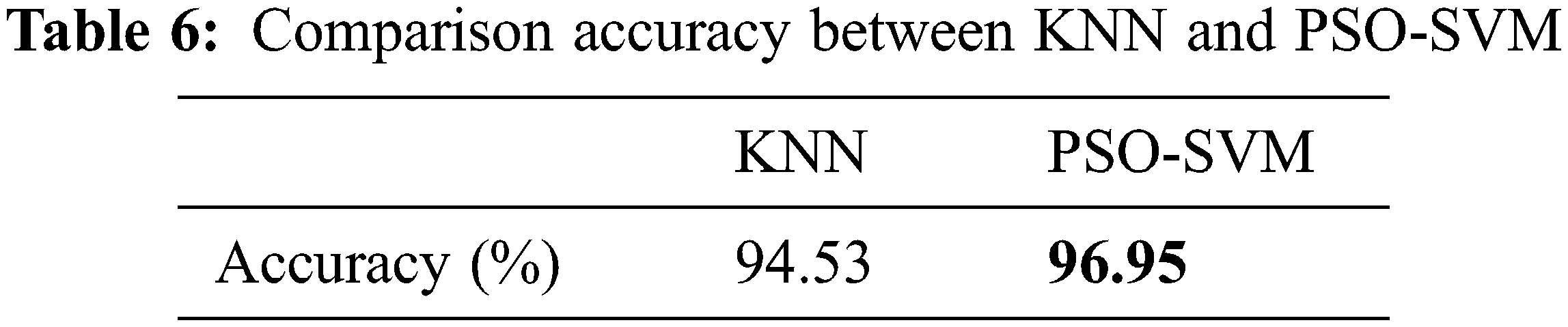
The simulation results illustrate that the PSO-SVM and KNN algorithms detect immobilization in various faults. The test result presented in Tab. 6 shows that the PSO-SVM method could diagnose errors correctly and efficiently with an accuracy of 96.95%. On the other hand, the KNN algorithm has a fault diagnosis with a precision of 94.53%. In this regard, we conclude that the PSO-SVM algorithm provides a better accuracy for the error classification, compared to the KNN algorithm.

7  Conclusions

In this paper a comparative study was made between the PSO-SVM and KNN methods for the classification of faults in a manipulator robot arm. In addition to the classification-based approach for fault detection, a fault detection method based on a dynamic model of the interaction of the SCARA robot was also introduced. Various parameters are considered as input vectors for classifying seven classes of faults within the manipulator. The diagnostic accuracy of the two classifiers was estimated using 63,000 samples from the associated database. The classification method by SVM has a strong capability of learning the characteristics of the system (manipulator), which avoids the problems of low exemplary and poor distinction of traditional manual uprooting of the characteristics, and improves the diagnostic accuracy of the characteristics faults. In order to improve the SVM method, a PSO algorithm has been proposed in this paper to perform automatic optimization of the SVM parameters, which facilitates the efficiency of optimization of these parameters. Extensive simulations were conducted to demonstrate the efficacy of the proposed method. The numerical optimization simulations were carried out based on 7 widely applied fault classes and simulation results indicated that the proposed PSO variant has better performance in terms of search accuracy and speed of convergence. The results also demonstrate that the PSO-SVM algorithm offers a more accurate diagnosis than the KNN algorithm. The SVM algorithm may be a promising technique to diagnose defects in robotic manipulators. In the future, it is recommended that the SVM algorithm be linked to other optimization techniques in order to achieve better results.

Acknowledgement: The authors acknowledge the financial support received from Taif University Researchers Supporting Project (Number TURSP-2020/122), Taif University, Taif, Saudi Arabia.

Funding Statement: This work was supported by Taif University Researchers Supporting Project (Number TURSP-2020/122), Taif University, Taif, Saudi Arabia.

Conflicts of Interest: The authors declare that they have no conflict of interest.

This work is licensed under a Creative Commons Attribution 4.0 International License, which permits unrestricted use, distribution, and reproduction in any medium, provided the original work is properly cited.