Intelligent Automation & Soft Computing DOI:10.32604/iasc.2023.028604
Article

Minimizing Total Tardiness in a Two-Machine Flowshop Scheduling Problem with Availability Constraints

Mohamed Ali Rakrouki1,2,*, Abeer Aljohani1, Nawaf Alharbe1, Abdelaziz Berrais2 and Talel Ladhari2

1Applied College, Taibah University, Saudi Arabia
2University of Tunis, Tunis, Tunisia
*Corresponding Author: Mohamed Ali Rakrouki. Email: mrakrouki@taibahu.edu.sa
Received: 13 February 2022; Accepted: 24 March 2022

Abstract: In this paper, we consider the problem of minimizing the total tardiness in a deterministic two-machine permutation flowshop scheduling problem subject to release dates of jobs and known unavailability periods of machines. The theoretical and practical importance of minimizing tardiness in flowshop scheduling environment has motivated us to investigate and solve this interested two-machine scheduling problem. Methods that solve this important optimality criterion in flowshop environment are mainly heuristics. In fact, despite the NP -hardness in the strong sense of the studied problem, to the best of our knowledge there are no approximate algorithms (constructive heuristics or metaheuristics) or an algorithm with worst case behavior bounds proposed to solve this problem. Thus, the design of new promising algorithms is desirable. We develop five metaheuristics for the problem under consideration. These metaheuristics are: the Particle Swarm Optimization (PSO), the Differential Evolution (DE), the Genetic Algorithm (GA), the Ant Colony Optimization (ACO) and the Imperialist Competitive Algorithm (ICA). All the proposed metaheuristics are population-based approaches. These metaheuristics have been improved by integrating different local search procedures in order to provide more satisfactory, especially in term of quality solutions. Computational experiments carried out on a large set of randomly generated instances provide evidence that the Imperialist Competitive Algorithm (ICA) records the best performances.

Keywords: Optimization; machine scheduling; flowshop; evolutionary algorithms

Nomenclature

1  Introduction

Scheduling has been often considered in the literature and has many practical issues in domains like manufacturing, computer processing, transportation, production planning, etc., In these domains, scheduling involves a decision-making process. It is concerned with allocating resources (machines) to tasks (jobs) throughout certain time periods with the goal of optimizing one or more objectives [1]. The resources can be machinery resources, human resources, CPU, Web server, etc. and referred to as “machines”. The tasks to be scheduled can be production operations, CPU tasks, timetabling activities, etc., and referred to as “jobs”. Basic scheduling problems consider that machines are available during the scheduling, or in practice all machines may be unavailable during several periods of time due to machine breakdown (known as stochastic) or a preventive maintenance (known as deterministic). In real-world scheduling problems, the total tardiness criterion is highly crucial, especially in industry, since failure to meet deadlines can harm company’s reputation and lead to a loss of confidence, increased costs, and customer loss.

This paper deals with the two-machine flowshop scheduling problem where the machines are subject to non-availability constraints and the jobs are subject to release dates. More precisely, we are given n jobs (j=1,...,n) to be scheduled in the same processing sequence on two machines M1 and M2 . Each job must be processed on machine M1 and on machine M2 during p1j and p2j time units, respectively. There exists a due date dj associated with the completion of each job and each job can not start before a release date rj . The aim is minimizing the total tardiness of jobs.

Moreover, the following assumptions are considered. Each machine Mi(i=1,2) is unavailable during hi periods of time (hole). The number of holes, their starting times and their finish times are known in advance. No two holes overlap on the same machine. The two machines can have the same holes. Zero, one or several holes can occur during the processing of one job. Job processing can be interrupted by a machine unavailability and resumed after.

Let Cj be the completion time of job j on machine M2 , the objective is to find a schedule which minimizes the total tardiness of the jobs ∑j=1n⁡Tj where Tj=max(0,Cj−dj) . According to the notation specified by Pinedo 2012 [1] and Lee [2], this problem is denoted F2,hlo∣r−a,rj∣∑Tj . It’s an extension of the F2∣∣∑Tj problem and known to be NP -hard in the strong sense [3].

The rest of this paper is organized as follows: A literature review is provided in Section 2. Section 3 discusses the five proposed metaheuristics. In Section 4, the experimental findings and the comparative analysis are discussed. Finally, conclusions are set out in Section 5.

2  Literature Review

This problem has been studied only once before, despite its theoretical and practical importance. Indeed, Berrais et al. [4] proposed a mixed-integer formulation as well as some constructive heuristics for the problem under consideration.

The m -machine flowshop ( F∣∣∑Tj ) has been widely studied in the literature. Kim [5] developed a branch-and-bound algorithm using some proposed lower bounds and a dominance rule. A tabu search algorithm with diversification, intensification, and neighborhood restriction were proposed by Armentano et al. [6] to solve the same problem. Hasija et al. [7] proposed a simulated annealing (SA) algorithm. Chung et al. [8] proposed an exact method based on a branch-and-bound algorithm. Ghassemi Tari et al. [9] proposed four heuristics based on cost over time and more after Ghassemi Tari et al. [10] proposed seven heuristic algorithms, based on shortest processing time (SPT) and earliest due date (EDD) rules and then modified and combined to develop others algorithms. Chung et al. [11] developed a genetic algorithm. Liu et al. [12] proposed five dispatching rules, and a constructive heuristic for the m -machine no-wait flowshop with total tardiness criterion ( Fm∣no−wait∣∑Tj ). Ghassemi Tari et al. [13] proposed some heuristic procedures for tardiness problem with intermediate due dates. Fernandez-Viagas et al. [14] as well as Karabulut [15] proposed some iterated-greedy-based algorithms for the F∣∣∑Tj .

Sen et al. [16] considered the two-machine problem ( F2∣∣∑Tj ) and developed a branch-and-bound procedure in many presented cases. Koulamas [17] developed a heuristic denoted by guaranteed accuracy shifting bottleneck algorithm. Schaller [18] treated the same problem and proposed three dominance conditions to improve some previously proposed ones, and then proposed a new dominance rule as well as a branch-and-bound algorithm. Kharbeche et al. [19] proposed an exact method based on mixed-integer programming models.

Schmidt [20] and Ma et al. [21] proposed good descriptions and details about availability constraints. Blazewicz et al. [22] proposed three heuristic methods as well as a simulated annealing algorithm for minimizing the makespan in the resumable case ( F2,hij∣r−a∣Cmax ). Ben Chihaoui et al. [23] proposed several lower and upper bounds and used them in a branch-and-bound algorithm to solve the two-machine no-wait problem subject to release dates under the non-resumable case ( F2,h1j∣nr−a,rj∣Cmax ) with only hole considered on each machine. Under the assumption of the non-availability on the first machine, Lee et al. [24] proposed a branch-and-bound algorithm with some dominance properties and lower bounds as well as heuristic algorithm. For the parallel machine problem, Lee et al. [25] proposed some dominance properties and lower bounds as well as a branch-and-bound algorithm for minimizing the total tardiness where the machines need preventive maintenance.

3  Evolutionary Algorithms

In this section, five evolutionary algorithms are described. These algorithms are combined with several local search procedures to take the advantages of rapid exploitation and global optimization.

3.1 Particle Swarm Optimization Algorithm

Particle Swarm Optimization (PSO) algorithm is an evolutionary meta-heuristic proposed by Kennedy et al. [26]. PSO is similar to genetic algorithms but it hasn’t neither crossover nor mutation operators. Instead, it uses randomness of real numbers and the global communication among the swarm particles. Since its introduction, PSO algorithm has been improved with different techniques and proposed for various problems [27–30].

A PSO algorithm consists of a population [X1t,X2t,...,XNt] of N particles. Each particle Xit(i=1,...,N) at iteration t of the algorithm is denoted Xit=[xi1t,xi2t,....,xint] corresponding to its position in the swarm. The quality of position is represented by a fitness (objective function value). At each iteration t , the velocity Vit=[vi1t,vi2t,...,vint] and the position of each particle Xit=[xi1t,xi2t,....,xint] are updated toward its current best position (Xi∗=[xi1∗,xi2∗,....,xin∗]) and the global best position (G∗=[g1∗,g2∗,....,gn∗]) in the swarm. So, at each step and for each particle, a new velocity value is calculated based on its current one. This new value is used to compute the next position of the particle in the swarm. This process is repeated until a termination condition is reached.

The inertia weight wt determines the impact of a particle’s previous velocity to its current one. A large weight directs the algorithm to a global search while a small weight implies a local search. According to Bansal et al. [31], good results can be found when inertia weight is from 0.9 down to 0.4 . This latter is updated at each iteration as wt=wt−1β , where β is a decrement factor (β=0.975) .

The velocity Vit=[vi1t,vi2t,...,vint] of each particle is updated according to:

vijt=wt−1vijt−1+c1r1(xij∗−xijt−1)+c2r2(gj∗−xijt−1);∀j=1,…,n (1)

where c1,c2 are the acceleration coefficients and r1,r2 two randomly generated constant drawn on [0..1]. Usually c1+c2≤4. In this algorithm, c1+c2=4 (empirically chosen values).

The position of each particle Xit=[xi1t,xi2t,….,xint] is updated as follows:

xijt=xijt−1+vijt;∀j=1,…,n (2)

Since real numbers are used in the particle representation, real numbers are transformed to a feasible solution (permutation). Two approaches are used in our algorithm:

The Smallest Position Value (SPV): It consists of transforming the real values Xit=[xi1t,xi2t,....,xint] to a permutation by sorting these values in ascending order. Example: X=[x1=0.24,x2=−0.12,x3=1.21,x4=−1.25] with π=(1,2,3,4) . After sorting, X=[x4=−1.25,x2=−0.12,x1=0.24,x3=1.21] so π=(4,2,1,3) .

The Biggest Position Value (BPV) have the same principle as SPV but the positions are sorted in descending order.

3.1.1 Particles Initialization

The population is initialized by generating randomly the initial position and velocity vectors for each particle. The initial position values Xi0=[xi10,xi20,...,xin0] are drawn uniformally on [xmin,xmax]=[−4.0,4.0] . The velocity Vi0=[vi10,vi20,...,vin0] of each particle Xi0 is generated randomly, namely vijt=[vmin,vmax]=[−4.0,4.0] .

In order to obtain a heterogeneous population, most of the particles are randomly generated while some particles are generated using five constructive heuristics Hi(i=1,2,3,4,5) developed by Berrais et al. [4].

3.1.2 Local Search Hybridization

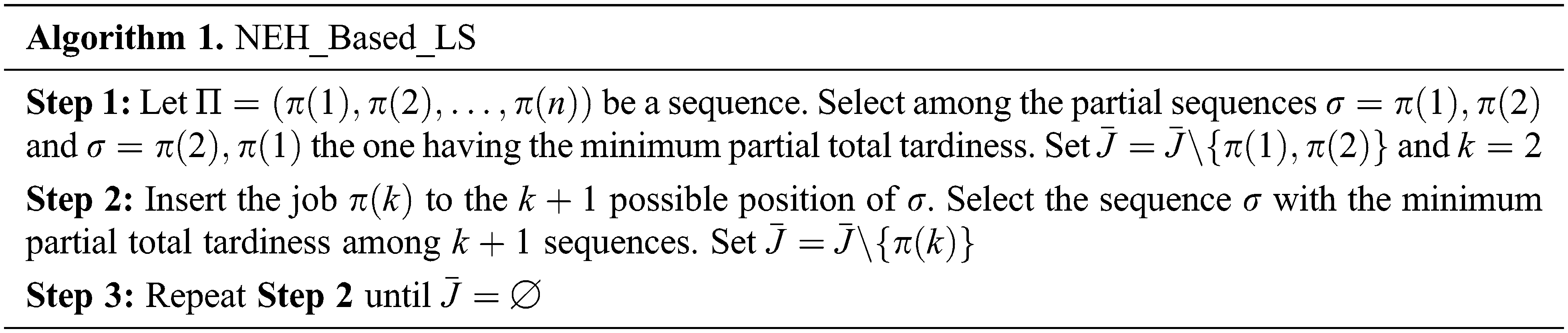
In order to produce high-quality solutions, a local search (LS) procedure is integrated to the PSO algorithm. The proposed local search is based on the Nawaz et al. (NEH) algorithm [32].

Let σ be a partial sequence of scheduled jobs and J¯ be the set of unscheduled jobs, this procedure can be described as follows:

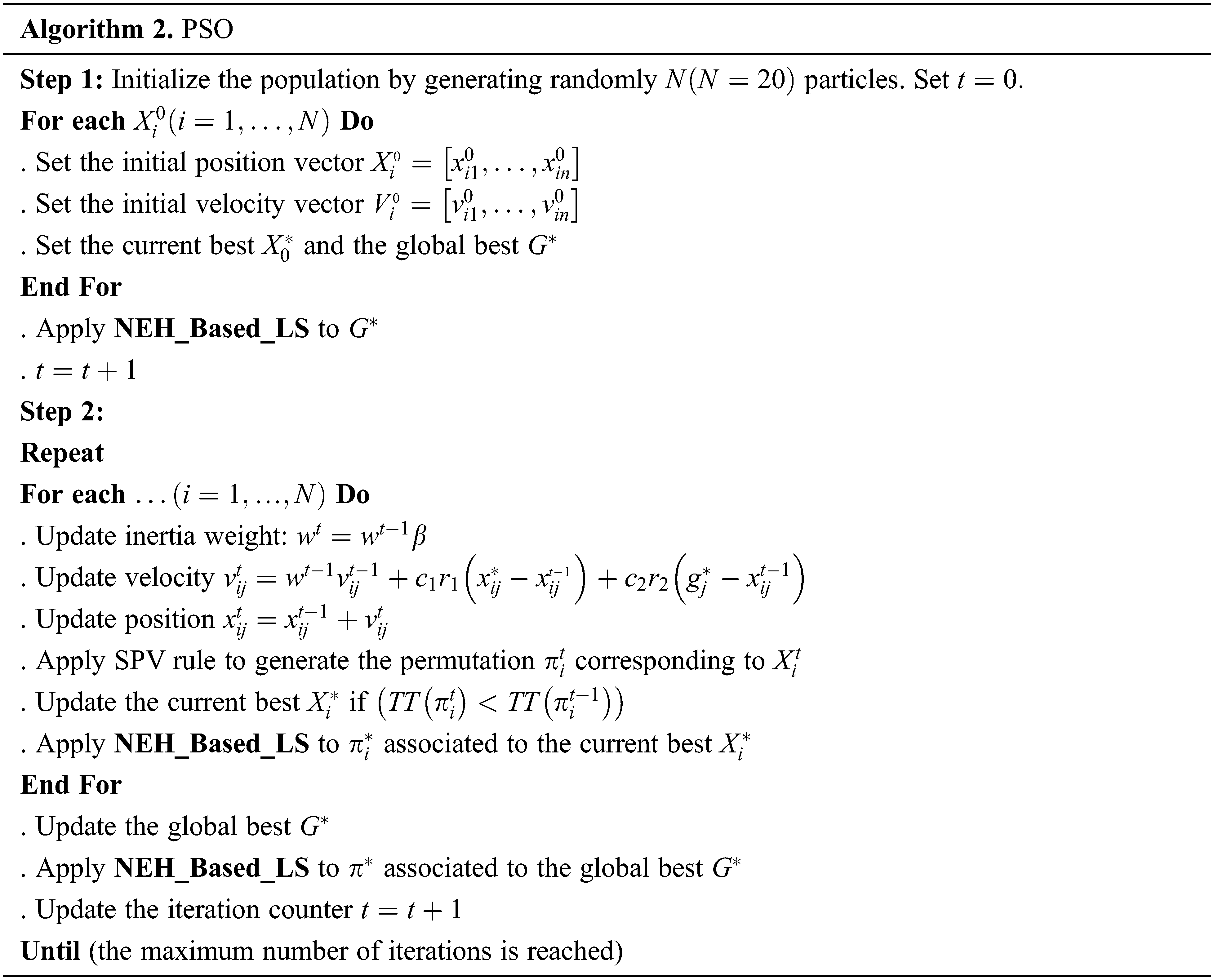
3.1.3 Pseudo-code of the proposed PSO algorithm

An outline of the proposed PSO is the following:

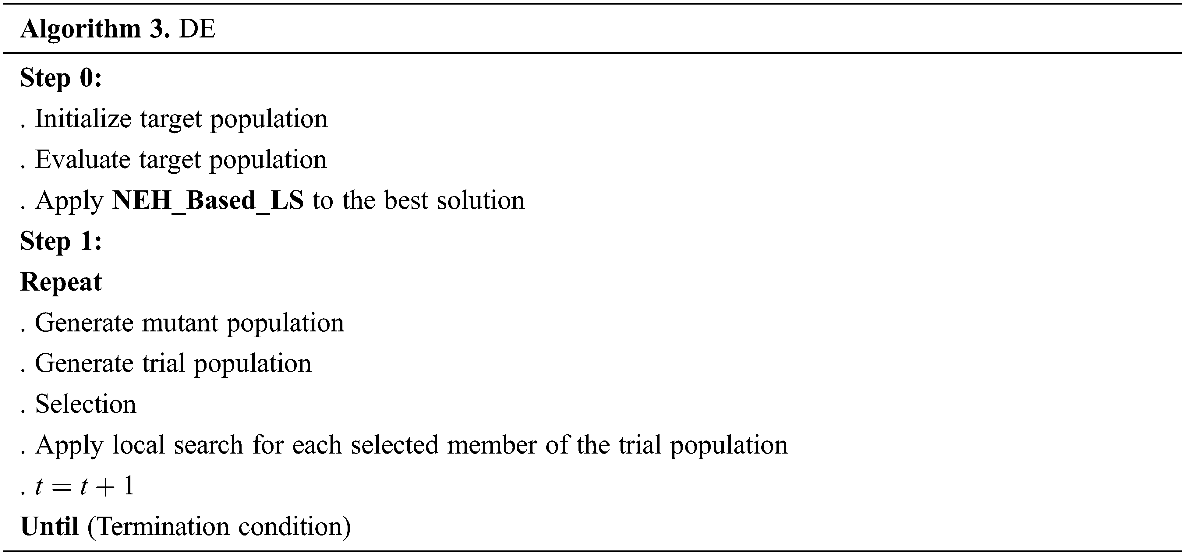
3.2 Differential Evolution Algorithm

Differential Evolution (DE) is an evolutionary algorithm firstly proposed by Storn et al. [33] for minimizing non differentiable continuous space functions. Like PSO, a DE algorithm is a population-based search meta-heuristic. It is one of the most powerful stochastic algorithms and it has been widely and successfully applied in many areas. DE algorithms were firstly designed to work with continuous variables. Then different strategies have been proposed to adapt the DE algorithm to optimize integer variables. Lampinen et al. [34] used a simple function to convert real numbers to integers. Onwubolu et al. [35] developed two strategies known as Forward Transformation (FT) and Backward Transformation (BT). Tasgetiren et al. [36] used the Smallest Position Value (SPV) rule inspired from random key representation encoding scheme of Beans [37].

In DE algorithm the first population is called target population. It consists of N randomly chosen chromosomes (solutions). Each solution Xi=[xi1,xi2,...,xin] is represented by a random floating-point numbers vector. As a mutation operator, two solutions are randomly chosen and the weighted difference between them is added to a third solution to generate a new population (called mutant population). After that, the crossover operator was applied. In this step, the mutated solutions obtained in the previous process are combined with the target population to generate a new one (known as trial population). Finally, the fitness value of the target and trial populations were compared using a selection operator to determine who can survive for the next generation. An outline of our proposed DE algorithm is the following:

3.2.1 Target Population

Our DE starts with the initialization of the target population Pt=[X1t,X2t,..,XNt] of N members. Each member Xit=[xi1t,xi2t,...,xint] at the iteration t is a vector of continuous random number xijt , where n is the number of jobs and xij0=xmin+(xmax−xmin)⋅rdj with r∈[0,1],xmin=−1 and xmax=1.

To find the corresponding permutation, H1,H2,H3,H4 and H5 are applied in order to generate the five first solutions and the best solution between the Smallest Position Value (SPV) and Biggest Position Value (BPV) for the remaining solutions. Then each member Xit in the target population is evaluated by computing the total tardiness.

3.2.2 Mutant Population Generation

A weighted difference between two randomly chosen members from the target population Xat and Xbt is added to a third one Xct (a≠b≠c∈[1,N]) to obtain the mutant population Vt=[V1t,V2t,...,VNt] where Vit=[vi1t,vi2t,...,vint] denotes a mutant individual. vijt is computed as in Onwubolu et al. [35]. Indeed, they have proved that is the best strategy for the total tardiness criterion. So, in our DE procedure Vit=Xat+F⋅(Xbt−Xct) as a mutant factor that controls the differential variation amplification (Xbt−Xct) . In our implementation F=0.5.

3.2.3 Trial Population Generation

Let Ut denotes the trial population with Ut=[U1t,U2t,...,UNt]. The Uit is the member of the trial population with Uit=[ui1t,ui1t,...,uint]. To generate this population, a crossover operator is applied as follows:

Let λ∈[1,n] be a random integer number, r∈[0,1] be a uniform random number, C∈[0,1] be a user-defined crossover constant, each element of Uit=[ui1t,ui1t,...,uint] is generated according the following equation:

uijt={uijtifr≤Corj=λxit−1otherwise (3)

The SPV rule is used to obtain the permutation and then evaluate each member Uit in the trial population by computing its total tardiness. In our implementation, λ is fixed at 0.05.

3.2.4 Selection

To make selection and determine the members who will survive for the next generation, the fitness of the member Xit is compared with the fitness of the member Uit:

Xit={Uitiff(π(Uit))<f(πit)Xit−1otherwise  (4)

3.2.5 Local Search Hybridization

A hybridization of our DE algorithm is proposed by integrating some local search procedures, in order to enhance its performance. Ten local search schemes are proposed and, in each iteration, only one is used according to a probability P . Given a permutation Π=(π(1),π(2),…,π(n)) , these procedures are the following:

•   Random_Exchange_LS: Generate two random positions i,j∈[1,n] with i≠j and then exchange π(i) and π(j).

•   Exchange_All_LS: Generate a random position i∈[1,n] and exchange π(i) with all k positions in the sequence Π with k∈[1,n], and k≠i .

•   Bloc_Exchange_LS: Decompose the sequence Π in n div blocs and exchange each job π(i) with its symmetric position s in the bloc sequence.

•   Symmetric_Exchange_LS: Exchange each job π(i) with its symmetric position (n−i+1) in the job permutation Π .

•   Intensive_Exchange_LS: Generate two random positions i and j with (i<j) and exchange each job π(k) in the sub-sequence (π(i),…,π(j)) with all the remaining jobs.

•   Insertion_LS: Remove a randomly chosen job π(i) and insert it at a new position j (i≠j) .

•   Circular_Insertion_LS: Place the job in the first position π(1) at the last position n and then shift the remaining jobs. This step is repeated (n−1) times.

•   Adjacent_Swap_LS: Starts from a randomly chosen position k and exchange π(k) with the job π(k+1) and then increment k by (k=k+2) . These steps are repeated until k=n−1 .

•   Bloc_Swap_LS: Decomposing the sequence in n div blocs and then exchange two adjacent jobs in the same bloc π(k) with the job π(k+1) .

•   NEH_Based_LS.

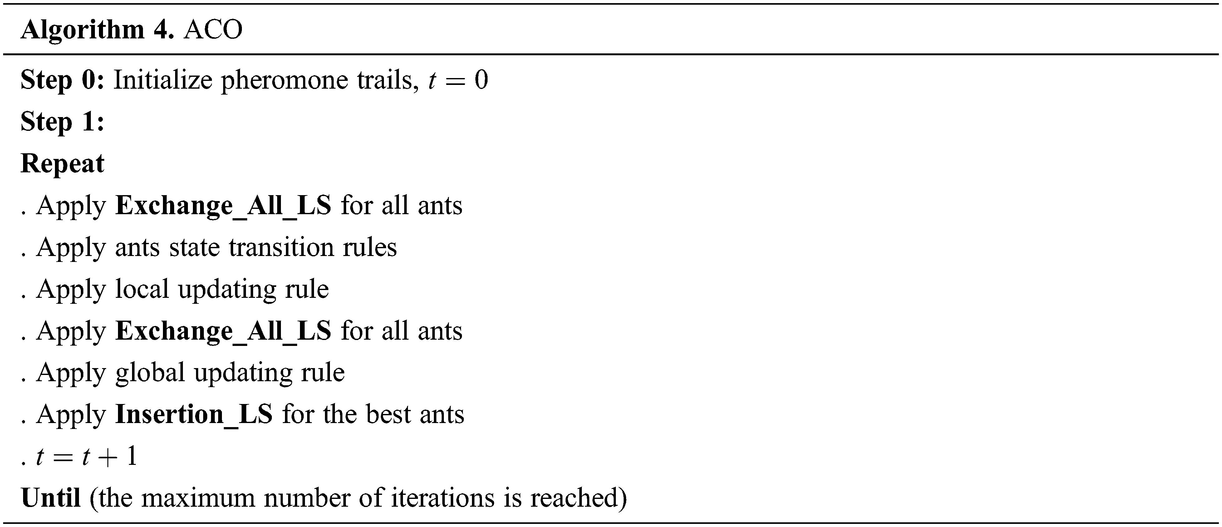
3.3 Ant Colony Optimization Algorithm

Ant Colony Optimization (ACO) is an evolutionary algorithm based on the behavior of ants. In order to mark some shortest path between ant nest and food that should be followed by other colony ants, these ants deposit a chemical substance called pheromone.

ACO algorithm has been proposed in the early nineties by Dorigo et al. [38]. This meta-heuristic belongs to ant colony algorithm family introduced by Dorigo [39] to solve the Travel Salesman Problem. Several variants of ACO algorithms have since been proposed to solve various optimization problems.

The outline of our ACO algorithm is as follows:

All the steps of our ACO are described as follows.

3.3.1 Pheromone Trails Initialization

The ACO algorithm starts by initializing the pheromone trails. Let N be the number of ants (population size), so initially N ants are randomly generated. Let Xit denotes the ith member in the population at the generation t with Xit=[xi1t,xi2t,...,xint] , n is the number of jobs and xijt is a continuous random number xij0=xmin+(xmax−xmin)⋅r with r∈[0,1],xmin=−1 and xmax=1. It is worth noting that for finding permutation the same method as our DE is used.

After that, three matrices are initialized:

•   The τ matrix of the pheromone density for each ant, where τij is the density of pheromone between two jobs i and j . All τij=τ0 where τ0 is the initial rate of pheromone, and τ0=1(1−r0)⋅Tbest where r0 is a random chosen constant and Tbest is the best fitness value found.

•   The δ matrix of the distance for each ant, where δij is the distance between two jobs i and j , and δij=p1j+p2j.

•   The η matrix of heuristic value for each ant, where ηij=1δij is the inverse of the distance between two jobs i and j .

3.3.2 The State Transition Rule

To move from job i to job j , the ants use a decision rule known as State Transition Rule (STR) or Pseudo-random Proportional Rule (PPR). The probability Pijt for an ant to move from job i to job j depends on a random variable q uniformly distributed over [0,1] , and a parameter q0 :

j={argmax(j∈πit){[τij]α[ηij]β}ifq≤q0PijtotherwisewithPijt={[τij]α[ηij]β∑j∈πit⁡[τij]α[ηij]βifj∈πit0otherwise  (5)

α and β are parameters controlling the relative importance of the pheromone vs. ηij=1/δij .

3.3.3 The Local Updating Rule

Local updating rule favors the exploration of other solutions to avoid premature convergence. This rule is performed after each step by all the ants as follows:

τij=(1−κ)⋅τij+κ⋅τ0  (6)

where κ∈[0,1] and τ0 are the decay coefficient and the initial value of the pheromone, respectively. Then for each ant Intensive_Exchange_LS is applied as local search procedure.

3.3.4 The Global Updating Rule

At the end of each tour, a global updating rule is applied only by the ant finding the shortest way as follows:

τij=(1−ρ)τij+ρ⋅Δτij  (7)

where Δτij=1Tbest if (i,j)∈π∗ with π∗ is the global best sequence, Tbest is the best fitness found, and ρ∈[0,1] is a pheromone evaporating parameter.

3.4 Imperialist Competitive Algorithm

Imperialist Competitive Algorithm (ICA) is an evolutionary algorithm introduced by Atashpaz-Gargari et al. [40]. It’s a population-based algorithm inspired by the imperialistic competition. The imperialism consists of expanding the powerful of a country (known as imperialist) by dominating others countries (called colonies) to take control of their resources. So, several imperialists compete for taking possession of colonies of each other. Each individual in the population is called country and can be imperialist or colony. All these colonies are divided among the imperialists according to their power to form empires. Then each colony start moving toward their relevant imperialist country. The total power of an empire depends mainly on the power of the imperialist country and has a negligible effect by the power of the colonies. After that the imperialistic competition between these empires starts and some empires increase their power. However, the powerless ones can’t increase their power and will be eliminated from the competition.

Our proposed ICA algorithm follows these steps:

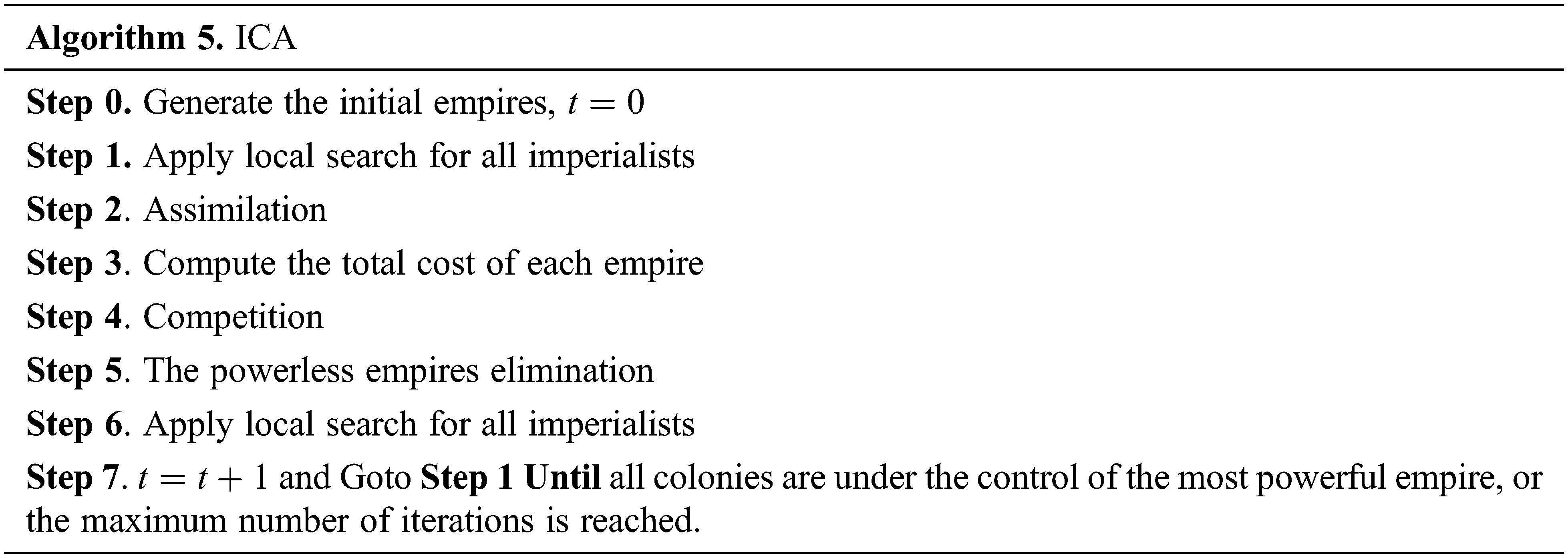
3.4.1 Initial Empires Generation

The ICA begins by generating the initial empires. Let N be the number of empires (the population size), and Nimp be the number of imperialists and Ncol be the number of colonies with N=Nimp+Ncol . So initially, N countries are randomly generated. Let C be a country is the set of N members with Ci=[X1i,X2i,..,XNi]. Let Xgi denotes the ith member in the population at the generation t with Xit=[xi1t,xi2,t...,xint] , n is the number of jobs and xijt is a continuous random number where xij0=xmin+(xmax−xmin)⋅r with r∈[0,1],xmin=−1 and xmax=1. To find permutation the same approach as in our DE is used.

Then the Nimp most powerful countries are selected as imperialists and the remaining Ncol countries as colonies. To generate the initial empires, the colonies among imperialists are divided based on their power. So, the initial number of colonies of each empire must be proportionate to its power. Then the normalized cost Φimp of an imperialist imp is defined by Φimp=φimp−max{φi} where φimp is the cost of the imperialist imp and Φimp its normalized cost, respectively.

Therefore, the normalized power Ψ of each imperialist presents the approximate number of colonies that should be possessed by that imperialist and is defined by:

Ψimp=|Φimp∑i=1Nimp⁡φi|  (8)

Also, the initial number of colonies of an empire imp is: Nimp=round{Ψimp⋅Ncol} . So, for each empire Nimp colonies are randomly selected.

3.4.2 Local Search Procedures

For each imperialist, one of the three previously defined local search procedures are applied randomly: Insertion_Suppression_LS, Intensive_LS and NEH_Based_LS.

3.4.3 Assimilation

The aim of this step is to move the colonies of an empire toward the imperialist. A procedure of perturbation (NEH_Based_L_S) is applied to the job permutation of the colony. If the colony’s cost is less than the imperialist’s cost then we exchange the position of this colony with the relative imperialist.

3.4.4 Total Cost Computing

After that the total cost of an empire is computed as follows. Let TCimp be the total cost of the impth empire and ξ be a positive number ξ∈[0,1] , the total cost is computed as follows:

TCimp=Cost(imperialistimp)+ξ⋅mean(Cost(Coloniesimp))  (9)

So, the value of the total cost depends on the power of imperialist, and the power of the colony can weakly affect this value if ξ have a large amount and can’t affect this value if ξ have a small amount.

3.4.5 Competition

In this step, each empire tries to possess and control the colonies of other empires. As a result of this competition, the colonies of powerless empires will be divided among other imperialists and will not necessarily be possessed by the most powerful empires. To model this competition, first each empire’s ownership likelihood is calculated according to its total cost.

Let NTCimp be the normalized total cost of the impth empire, TCimp its total cost, and Pimp be the possession probability of each empire, then NTCimp=TCimp−max{TCi},i={1,2,...,Nimp} and Pimp=|NTCimp∑i=1Nimp⁡NTCi| .

Then the vector P=[P1,P2,...,PNimp] , the vector R=[r1,r2,...,rNimp] with ri∈[0,1] , and the vector D=P−R[P1−r1,P2−r2,...,PNimp−rNimp] are computed. So, the empire with the maximum value of Di will take the colonies. If after some iterations, the powerless empires lose all their colonies so they will be eliminated.

3.5 Genetic Algorithm

Genetic Algorithm (GA) is an evolutionary algorithm that have been successfully applied to different complex combinatorial optimization problems such as scheduling problems, knapsack problems, traveling salesman problem, etc. The GAs were introduced by Holland [41] and are inspired from Darwin’s theory of evolution. So, GA approach is based on natural evolution techniques, such as selection, crossover and mutation.

GA is a population-based algorithm, so each member in the population is called chromosome or solution. Starting from an initial population, the goal is to create new populations with better solutions after some iterations (called generation). In each generation, the fitness of every chromosome in the population is computed by an evaluation function to select the most fitted individuals from the current population. Then some genetic operators such as crossover and mutation are applied to these selected chromosomes. This process is repeated until the satisfaction of a termination condition.

To solve our problem, a GA hybridized with local search procedures (known as genetic local search GLS) is used. This algorithm has been developed initially for the two-machine flowshop problem where the objective is to minimize the total completion time [42].

We recall here the pseudo-code of the GLS algorithm.

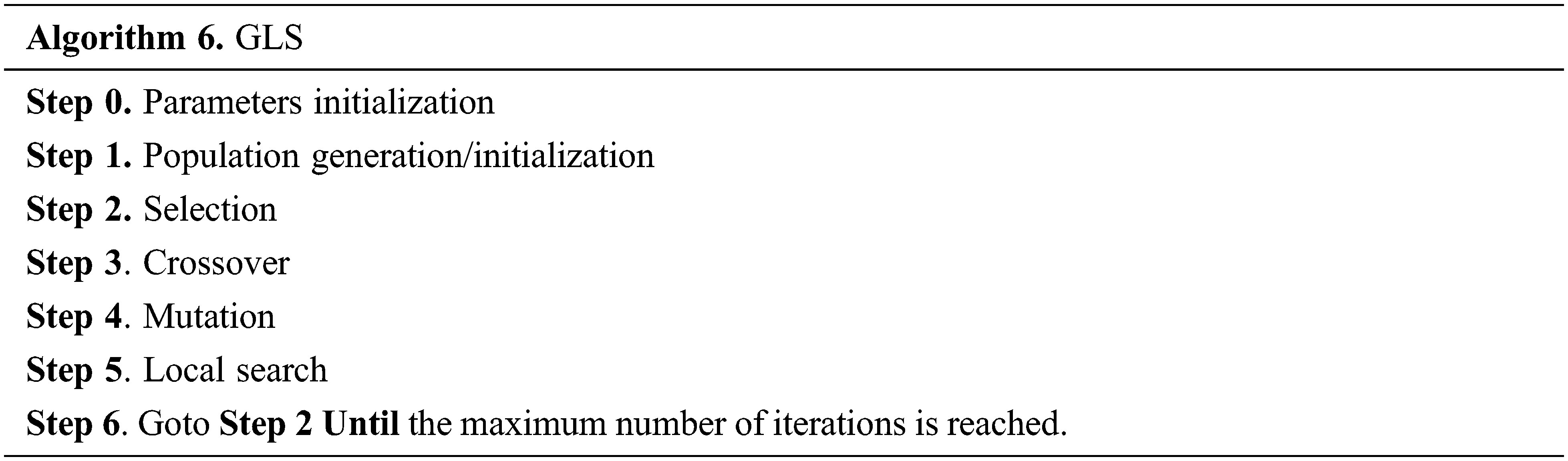
We The above procedure is adapted as follows. The initial population consists of M solutions. M−1 solutions are randomly generated while a single one is generated using H5 developed by Berrais et al. [4]. M is referred to as the population size. The fitness function consists on computing the total tardiness of a given solution.

4  Experimental Results

In order to evaluate the empirical performance of the proposed algorithms, a large set of computational tests have been undertaken. All these procedures were implemented in C and run on an Intel Core i5 PC (3.60 GHz) with 8 GB RAM.

4.1 Test Problems

Our proposed algorithms were tested on different problem sizes n∈{10,20,30,40,50,60,70,80, 90,100,200,300} . The processing times and the release dates are uniformly distributed on [1,100] and [0,∑j=1n⁡p1j2] , respectively. The due dates dj are generated using the scheme of [43] as follows: dj=rj+⌊f⋅(p1j+p2j)2⌋ where the due date slack factor f where generated from a discrete uniform distribution on [1−T−R2,1−T+R2] , and T and R are the tardiness factors of jobs T∈{1.5,2.5,3.5} , and the dispersion factor of due dates R∈{0.2,0.4,0.6} , respectively. By varying T and R , problem classes are obtained. For each class, instances were randomly generated for a total of test problems. Moreover, to consider the non-availability of machines, holes are randomly generated on each machine.

After an experimental study of the different parameters of our proposed algorithms, the following settings have been used to achieve high-quality solutions:

- PSO: N=20,c1=2,c2=2,vmin=−4,vmax=4,xmin=−4,xmax=4,β=0.975,w=0.9

- DE: N=20,xmin=−1,xmax=1,F=0.5,λ=0.05

- ACO: N=20,xmin=−1,xmax=1,α=0.1,β=0.1,φ=0.1,ρ=0.1

- GLS: The same parameters as in [42]

- ICA: N=150,Nimp=10,Ncol=140,ξ=0.05

For all algorithms, the maximum number of iterations is fixed experimentally according to the size of the problem ( n×50 ).

4.2 Performance of the Proposed Algorithms

To compare our algorithms’ performance, the average relative percentage deviation (ARPD) from the best-known solution is used. This percentage deviation is defined as ARPD=[UB−UB∗UB∗]×100 , where UB is the solution provided by PSO, DE, ACO, GLS or ICA and UB∗=min(UBi);(i=1,...,5) .

Tabs. 1 and 2 summarize the results of the computational experiments.

The analysis with respect to the problem size in Tab. 1 clearly reveals that the best results among all tested algorithms are found by the proposed ICA algorithm. In fact, in comparison to the remaining meta-heuristics this algorithm provides lower values of ARPD, for all problem sizes. Among the tested problems, ICA gives the best solutions for instances. It can solve very large instances with up to jobs within a moderate CPU time. The average time in all instances of jobs was 1628.9 s. It can see that the average CPU time grew significantly as the number of jobs increased, especially for the ICA and GLS algorithms. This is due to the fact that the number of jobs directly increases the number of iterations of the algorithms and thereby increasing the computation time.

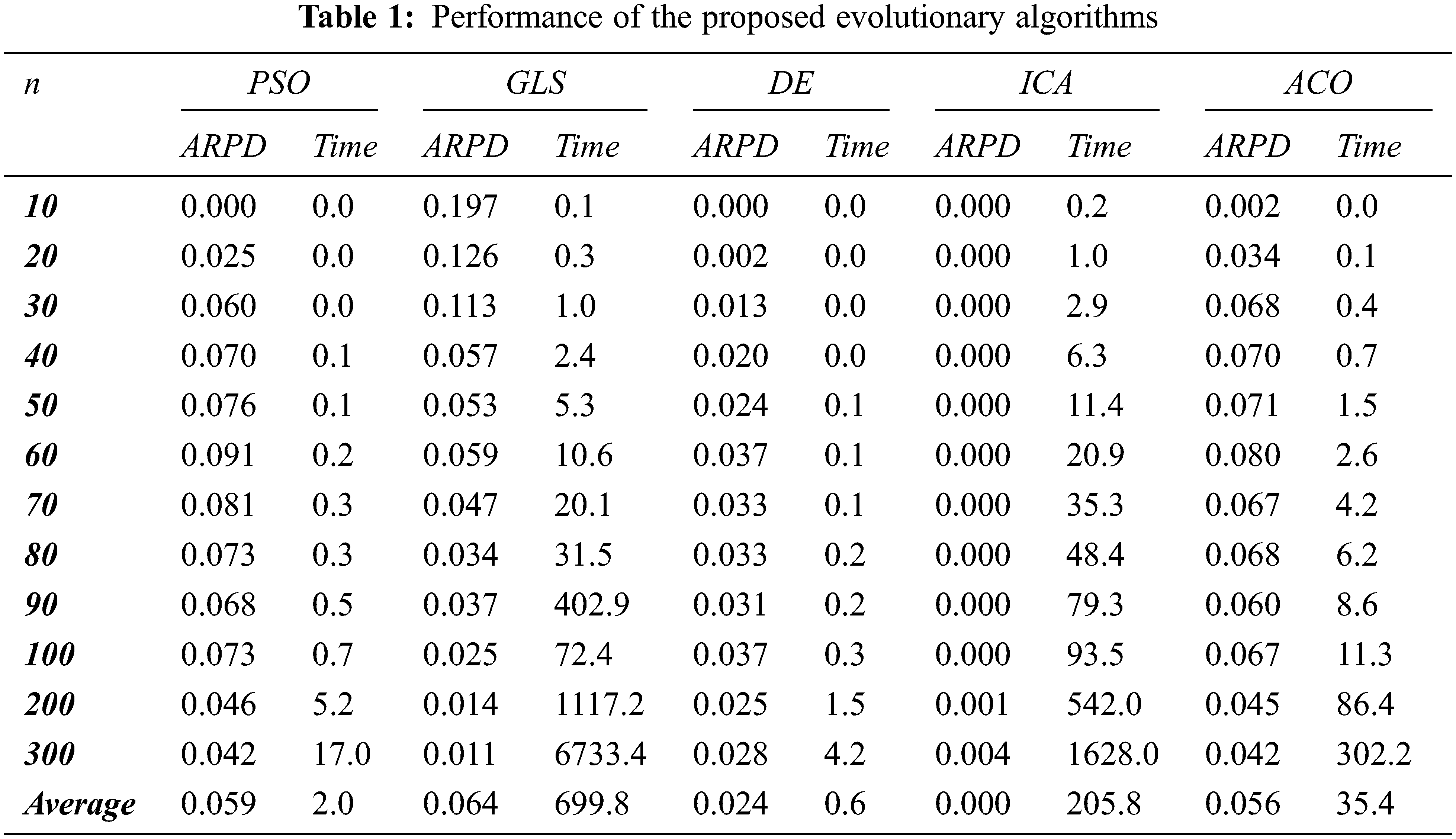
Regarding the computational results of the GLS algorithm, we observe that it gives very good results for large size problems ( n>90 ). In fact, the performance of GLS algorithm draws near significantly from the ICA algorithm for n>200 . Unfortunately, it shows the worst results for small size problems ( n≤30 ). For n=10 , all the proposed algorithms, except the GLS, present the best performances in term of ARPD and the DE algorithm shows the best CPU time ( 0.005 s). Furthermore, the DE algorithm shows better results than GLS for small and medium size instances ( n≤90 ). Also, we observe that in term of ARPD no significant differences between the PSO and ACO algorithms were found, particularly for large size instances ( n≥200 ).

Tab. 2 shows the ARPD of the proposed algorithms with respect to the combinations for the values of T and R . Our computational experience shows that the performance of the algorithms was affected considerably by the tardiness factor T . In fact, we observe that the ARPD increases when the tardiness factor T increases. The proposed algorithms were able to provide a lower ARPD for the instances which present lower tardiness factor ( T=1.5 ).

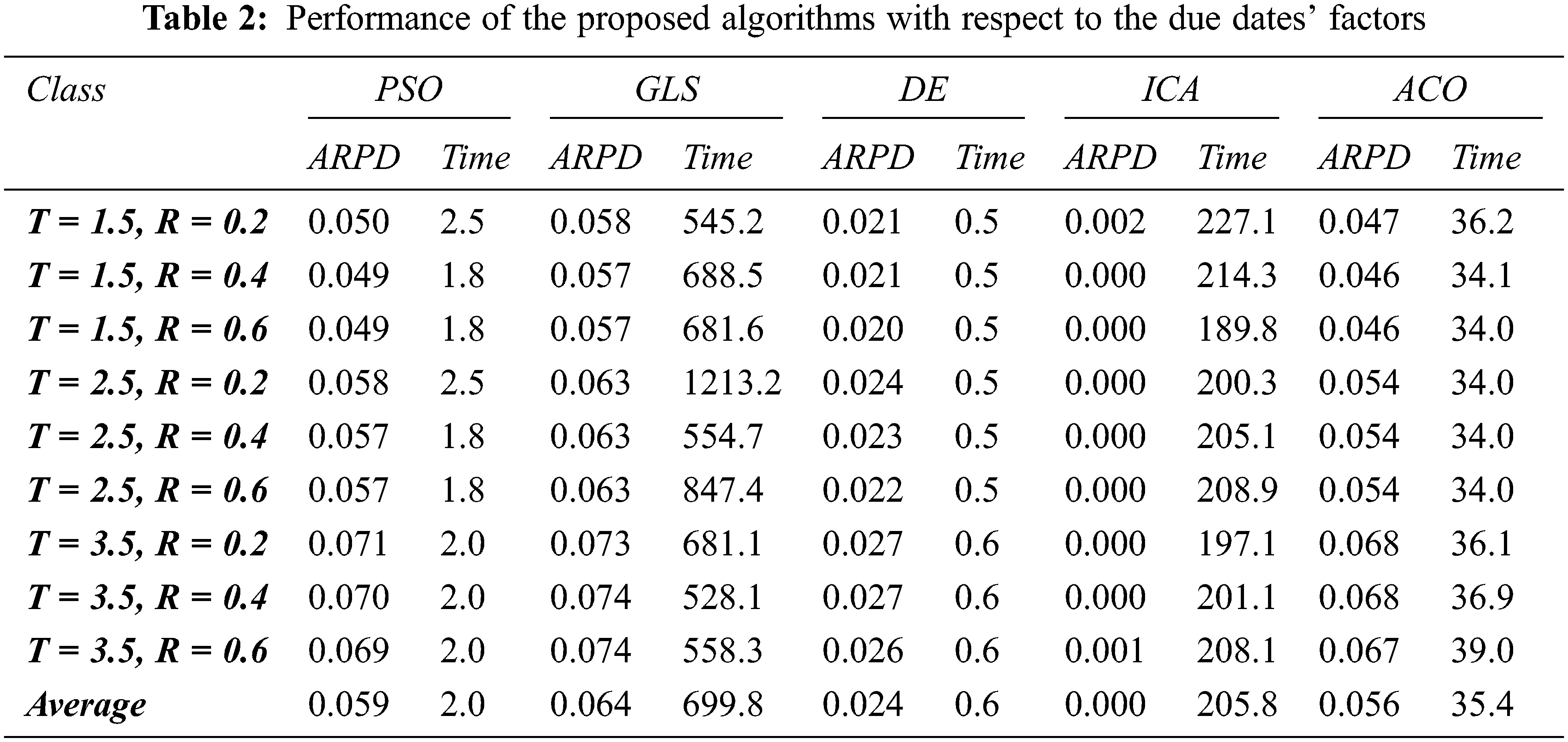
Regarding the due date range factor R , the results reveals that the ARPD of the proposed algorithms was slightly affected. Also, we observe the same remark for the CPU time except for the GLS algorithm. In fact, for this meta-heuristic the computation time increases considerably in particular for the ( T=2.5,R=0.2 ) and ( T=2.5,R=0.6 ) problem classes.

5  Conclusions

In this paper, we have proposed five evolutionary algorithms developed to minimize the total tardiness in a two-machine flowshop scheduling problem where the machines and jobs are subject to non-availability constraints and unequal release dates, respectively. To avoid the rapid convergence of these algorithms and in order to derive high-quality solutions, we proposed a hybridization of our algorithms with several local search procedures. Computational tests provide strong evidence, on the tested instances, that the Imperialist Competitive Algorithm (ICA) outperforms all the proposed population-based approaches.

Funding Statement: The authors received no specific funding for this study.

Conflicts of Interest: The authors declare that they have no conflicts of interest to report regarding the present study.

References

 1.  M. L. Pinedo, Scheduling: theory, algorithms, and systems, 4th ed., New York, USA: Springer, 2012. [Google Scholar]

 2.  C. Y. Lee, “Minimizing the makespan in the two-machine flowshop scheduling problem with an availability constraint,” Operations Research Letters, vol. 20, no. 3, pp. 129–139, 1997. [Google Scholar]

 3.  J. K. Lenstra, A. H. Rinnooy Kan and P. Brucker, “Complexity of machine scheduling problems,” Annals of Discrete Mathematics, vol. 1, no. C, pp. 343–362, 1977. [Google Scholar]

 4.  Berrais, M. A. Rakrouki and T. Ladhari, “Minimizing total tardiness in two-machine machine permutation flowshop problem with availability constraints and subject to release dates,” in Proc. of the 14th Int. Workshop on Project Management and Scheduling, Munchen, Germany, pp. 32–35, 2014. [Google Scholar]

 5.  Y. D. Kim, “Minimizing total tardiness in permutation flowshops,” European Journal of Operational Research, vol. 85, no. 3, pp. 541–555, 1995. [Google Scholar]

 6.  V. A. Armentano and D. P. Ronconi, “Tabu search for total tardiness minimization in flowshop scheduling problems,” Computers and Operations Research, vol. 26, no. 3, pp. 219–235, 1999. [Google Scholar]

 7.  S. Hasija and C. Rajendran, “Scheduling in flowshops to minimize total tardiness of jobs,” International Journal of Production Research, vol. 42, no. 11, pp. 2289–2301, 2004. [Google Scholar]

 8.  C. S. Chung, J. Flynn and Ö. Kirca, “A branch and bound algorithm to minimize the total tardiness for m-machine permutation flowshop problems,” European Journal of Operational Research, vol. 174, no. 1, pp. 1–10, 2006. [Google Scholar]

 9.  F. Ghassemi Tari and L. Olfat, “COVERT based algorithms for solving the generalized tardiness flow shop problems,” Journal of Industrial and Systems Engineering, vol. 2, no. 3, pp. 197–213, 2008. [Google Scholar]

10. F. Ghassemi Tari and L. Olfat, “A set of algorithms for solving the generalized tardiness flowshop problems,” Journal of Industrial and Systems Engineering, vol. 4, no. 3, pp. 156–166, 2010. [Google Scholar]

11. C.-S. Chung, J. Flynn, W. Rom and P. Staliński, “A genetic algorithm to minimize the total tardiness for m-machine permutation flowshop problems,” Journal of Entrepreneurship, Management and Innovation, vol. 8, no. 2, pp. 26–43, 2012. [Google Scholar]

12. G. Liu, S. Song and C. Wu, “Some heuristics for no-wait flowshops with total tardiness criterion,” Computers and Operations Research, vol. 40, no. 2, pp. 521–525, 2013. [Google Scholar]

13. F. Ghassemi Tari and L. Olfat, “Heuristic rules for tardiness problem in flow shop with intermediate due dates,” International Journal of Advanced Manufacturing Technology, vol. 71, no. 1–4, pp. 381–393, 2014. [Google Scholar]

14. V. Fernandez-Viagas, J. M. Valente and J. M. Framinan, “Iterated-greedy-based algorithms with beam search initialization for the permutation flowshop to minimise total tardiness,” Expert Systems with Applications, vol. 94, no. 3, pp. 58–69, 2018. [Google Scholar]

15. K. Karabulut, “A hybrid iterated greedy algorithm for total tardiness minimization in permutation flowshops,” Computers and Industrial Engineering, vol. 98, no. 4, pp. 300–307, 2016. [Google Scholar]

16. T. Sen, P. Dileepan and J. N. Gupia, “The two-machine flowshop scheduling problem with total tardiness,” Computers and Operations Research, vol. 16, no. 4, pp. 333–340, 1989. [Google Scholar]

17. C. Koulamas, “A guaranteed accuracy shifting bottleneck algorithm for the two-machine flowshop total tardiness problem,” Computers and Operations Research, vol. 25, no. 2, pp. 83–89, 1998. [Google Scholar]

18. J. Schaller, “Note on minimizing total tardiness in a two-machine flowshop,” Computers and Operations Research, vol. 32, no. 12, pp. 3273–3281, 2005. [Google Scholar]

19. M. Kharbeche and M. Haouari, “MIP models for minimizing total tardiness in a two-machine flow shop,” Journal of the Operational Research Society, vol. 64, no. 5, pp. 690–707, 2013. [Google Scholar]

20. G. Schmidt, “Scheduling with limited machine availability,” European Journal of Operational Research, vol. 121, no. 1, pp. 1–15, 2000. [Google Scholar]

21. Y. Ma, C. Chu and C. Zuo, “A survey of scheduling with deterministic machine availability constraints,” Computers and Industrial Engineering, vol. 58, no. 2, pp. 199–211, 2010. [Google Scholar]

22. J. Blazewicz, J. Breit, P. Formanowicz, W. Kubiak and G. Schmidt, “Heuristic algorithms for the two-machine flowshop with limited machine availability,” Omega, vol. 29, no. 6, pp. 599–608, 2001. [Google Scholar]

23. F. Ben Chihaoui, I. Kacem, A. B. Hadj-Alouane, N. Dridi and N. Rezg, “No-wait scheduling of a two-machine flow-shop to minimise the makespan under non-availability constraints and different release dates,” International Journal of Production Research, vol. 49, no. 21, pp. 6273–6286, 2011. [Google Scholar]

24. J. Y. Lee and Y. D. Kim, “Minimizing total tardiness in a two-machine flowshop scheduling problem with availability constraint on the first machine,” Computers and Industrial Engineering, vol. 114, pp. 22–30, 2017. [Google Scholar]

25. J. Y. Lee, Y. D. Kim and T. E. Lee, “Minimizing total tardiness on parallel machines subject to flexible maintenance,” International Journal of Industrial Engineering: Theory Applications and Practice, vol. 25, no. 4, pp. 472–489, 2018. [Google Scholar]

26. J. Kennedy and R. C. Eberhart, “Discrete binary version of the particle swarm algorithm,” in Proc. of the IEEE Int. Conf. on Systems, Man and Cybernetics, Orlando, FL, USA, 5, pp. 4104–4108, 1997. [Google Scholar]

27. X. Zhang, W. Zhang, W. Sun, X. Sun and S. K. Jha, “A robust 3-D medical watermarking based on wavelet transform for data protection,” Computer Systems Science and Engineering, vol. 41, no. 3, pp. 1043–1056, 2022. [Google Scholar]

28. H. Moayedi, M. Mehrabi, M. Mosallanezhad, A. S. A. Rashid and B. Pradhan, “Modification of landslide susceptibility mapping using optimized PSO-ANN technique,” Engineering with Computers, vol. 35, no. 3, pp. 967–984, 2019. [Google Scholar]

29. H. Jiang, Z. He, G. Ye and H. Zhang, “Network intrusion detection based on PSO-Xgboost model,” IEEE Access, vol. 8, pp. 58392–58401, 2020. [Google Scholar]

30. M. A. Shaheen, H. M. Hasanien and A. Alkuhayli, “A novel hybrid GWO-PSO optimization technique for optimal reactive power dispatch problem solution,” Ain Shams Engineering Journal, vol. 12, no. 1, pp. 621–630, 2021. [Google Scholar]

31. J. C. Bansal, M. Arya and K. Deep, “A nature inspired adaptive inertia weight in particle swarm optimization,” International Journal of Artificial Intelligence and Soft Computing, vol. 4, no. 2–3, pp. 228, 2014. [Google Scholar]

32. M. Nawaz, E. E. Enscore and I. Ham, “A heuristic algorithm for the m-machine, n-job flow-shop sequencing problem,” Omega, vol. 11, no. 1, pp. 91–95, 1983. [Google Scholar]

33. R. Storn and K. Price, “Differential evolution-a simple and efficient heuristic for global optimization over continuous spaces,” Journal of Global Optimization, vol. 11, no. 4, pp. 341–359, 1997. [Google Scholar]

34. J. Lampinen and I. Zelinka, “Mechanical engineering design optimization by differential evolution,” in New Ideas in Optimization, D. Corne, M. Dorigo, F. Glover (eds.UK: McGraw-Hill, pp. 127–146, 1999. [Google Scholar]

35. G. Onwubolu and D. Davendra, “Scheduling flow shops using differential evolution algorithm,” European Journal of Operational Research, vol. 171, no. 2, pp. 674–692, 2006. [Google Scholar]

36. M. F. Tasgetiren, Y. C. Liang, M. Sevkli and G. Gencyilmaz, “A particle swarm optimization algorithm for makespan and total flowtime minimization in the permutation flowshop sequencing problem,” European Journal of Operational Research, vol. 177, no. 3, pp. 1930–1947, 2007. [Google Scholar]

37. J. Beans, “Genetics and random keys for sequencing and optimization,” INFORMS Journal on Computing, vol. 6, no. 2, pp. 154–160, 1993. [Google Scholar]

38. M. Dorigo and L. M. Gambardella, “Ant colony system: a cooperative learning approach to the traveling salesman problem,” IEEE Transactions on Evolutionary Computation, vol. 1, no. 1, pp. 53–66, 1997. [Google Scholar]

39. M. Dorigo, “Optimization, learning and natural algorithms,” Ph.D. dissertation, Polytechnic University of Milan, Italy, 1992. [Google Scholar]

40. E. Atashpaz-Gargari and C. Lucas, “Imperialist competitive algorithm: An algorithm for optimization inspired by imperialistic competition,” in Proc. 2007 IEEE Congress on Evolutionary Computation, Singapore, pp. 4661–4667, 2007. [Google Scholar]

41. J. H. Holland, Adaptation in natural and artificial systems: an introductory analysis with applications to biology, control, and artificial intelligence. USA: University of Michigan Press, 1992. [Google Scholar]

42. T. Ladhari and M. A. Rakrouki, “Heuristics and lower bounds for minimizing the total completion time in a two-machine flowshop,” International Journal of Production Economics, vol. 122, no. 2, pp. 678–691, 2009. [Google Scholar]

43. Y. D. Kim, “A new branch and bound algorithm for minimizing mean tardiness in two-machine flowshops,” Computers and Operations Research, vol. 20, no. 4, pp. 391–401, 1993. [Google Scholar]

This work is licensed under a Creative Commons Attribution 4.0 International License, which permits unrestricted use, distribution, and reproduction in any medium, provided the original work is properly cited.