DOI:10.32604/iasc.2023.027248
| Intelligent Automation & Soft Computing DOI:10.32604/iasc.2023.027248 | |
| Article |
Intelligent Deployment Model for Target Coverage in Wireless Sensor Network
Department of ECE, National Engineering College, Kovilpatti, Tamilnadu, India
*Corresponding Author: K. Subramanian. Email: subramaniankrishnan83@gmail.com
Received: 13 January 2022; Accepted: 24 February 2022
Abstract: Target coverage and continuous connection are the major recital factors for Wireless Sensor Network (WSN). Several previous research works studied various algorithms for target coverage difficulties; however they lacked to focus on improving the network’s life time in terms of energy. This research work mainly focuses on target coverage and area coverage problem in a heterogeneous WSN with increased network lifetime. The dynamic behavior of the target nodes is unpredictable, because the target nodes may move at any time in any direction of the network. Thus, target coverage becomes a major problem in WSN and its applications. To solve the issue, this research work is motivated to design and develop an intelligent model named Distributed Flexible Wheel Chain (DFWC) model for efficient target coverage and area coverage in WSN applications. More number of target nodes is covered by minimum number of sensor nodes that can improve energy efficiency. To be specific, DFWC motivated at obtaining lesser connected target coverage, where every target is available in the monitoring area is covered by a smaller number of sensor nodes. The simulation results show that the proposed DFWC model outperforms the existing models with improved performance.
Keywords: WSN; target coverage; DFWC; network coverage
One of the emerging networks which can configure automatically is the Wireless Sensor Network (WSN), have an undefined number of sensor nodes connected logically and physically with the help of various communication mediums. Various WSN applications have deployed different kinds of sensors for monitoring purposes in a deterministic manner. Sensors are the most important component of any programmed system. Sensor nodes are distributed in a defined region to be watched [1]. Sensors can sense, gather data, process and perform the assigned tasks. Deploying the sensor in the defined region is a crucial factor that should satisfy the coverage and lifetime of WSN [2]. The application domain of target coverage in WSN involves military [3], disaster management [4], target monitoring [5], agriculture, surveillance monitoring [6] and intruder detection, etc [7]. Due to the target node’s mobility, speed, sensing region, coverage area, most of the target nodes cannot be covered at various scenarios like restricted sensing range, the distance among the sensor nodes and target nodes.
In target monitoring, most of the targets can be monitored/sensed only within a determined distance. The sensors are restricted with a sensing range as Sr and it is located at a distance SdistSdist(Sdist ≤ Sr) from the target location. In the case of heterogeneous WSN, the surveillance applications can have different types of sensors with various behaviors such as sensing ability, power utilization, battery limit and etc. Various earlier research works have assumed that the range of sensing and communication follows a binary disk model, whereas this model is not suitable for reality. This work considers a real-time application model for the range of sensing and communication of the nodes. Particularly, for easy controllability of the problem, this paper discussed a chain-link circular model with various range of sensing and communication.
Network coverage is quickly becoming one of the most critical variables influencing wsn service quality. Sensors can cover targets inside that coverage area when deployed, and if all sensors, target location, and coverage areas are known, the coverage relationship can be determined. The purpose of the coverage challenge is to find a subset of the sensor and extend its life while maintaining the original remaining resources’ life limit and overall power consumption in mind. The Voronoi diagram feature can help to simplify decision-making while enhancing target coverage.
In WSN, the target coverage, area coverage and connectivity are the major factors to be considered. This research work focused on target coverage and area coverage. Target coverage is monitoring a set of target nodes using a set of sensor nodes. If any node fails while monitoring, it disconnects the entire network communication. Applications need η-coverage that may occur in specific applications like the military, it requires a stronger environmental monitoring ability. This kind of problem can be created as a decision-making problem, where its aim is to determine distance among the sensor nodes and the target nodes not changing, the target is covered by the pre-assigned number sensors. When the target moves then the sensors also move at the same speed. The target coverage problem should ensure the network is reliable and accurate. The rest of the paper is as follows. The second section explains how efforts were made to strengthen target coverage activities. Section 3 includes a few instances of related work. Section 4 discusses the proposed approach. Section 5 investigates the efficacy of the proposed strategy. Finally, in Part 6, this article concludes.
Most of the target coverage applications require a centralized mechanism for forwarding the observed data to the destinations. It takes more energy consumption for communication and data transmission. But a distributed mechanism enables each node to decide its own task and can change its mode accordingly. Comparing with the centralized mechanism, the distributed mechanism consumes lesser energy and increase the performance as well. Hence this paper proposed the Distributed Flexible Wheel Chain (DFWC) model as a distributed algorithm, as it is highly suitable for large-scale surveillance environments. The main contribution of the paper is given as follows.
❖ Design and implement a distributed FWC algorithm for target coverage
❖ Illustrate multiple scenarios for solving the target coverage problem and to maintain DFWC continuously and constantly, so as to assure network reliability and accuracy.
❖ FWC is distributed so that it can be implemented for any large-scale heterogeneous network applications.
❖ Balancing the load, range of sensing and communication, DFWC can manage the sensing ability, energy and target coverage efficiently.
This paper provides the following scenarios towards illustrating the target coverage problem which has been solved. The overall flow of the proposed model is given in Fig. 1.
❖ Single Static Target with Multi-Static Sensor Nodes (SSTMSSN).
❖ Multi Static Target with Multi-Static Sensor Nodes (MSTMSSN).
❖ Single-Dynamic Target with Multi-Dynamic Sensor Nodes (SDTMDSN).
❖ Multi-Dynamic Target with Multi-Dynamic Sensor Nodes (MDTMDSN).
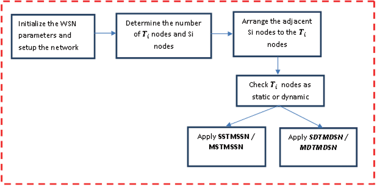
Figure 1: Overall flow of DFWC model
Target and area coverage, continuous connectivity is the major factors to be considered as the major and necessary problems in WSN applications. The target coverage problem either covers the target continuously without any break, cover the specific target area by deploying minimum sensor nodes and verify the area and target is covered well. Nowadays, target coverage and connectivity problems have paid high attention to the surveillance industry. To provide better and efficient methodology, several algorithms and methodologies have been proposed in the earlier research works. For example, the author in [8] deployed a collection of sensor nodes randomly and uniformly distributed in a static geometry and proves the required area coverage. Though, the main drawback of this method is, it is not really always. One of the recent research works has used the robotics group for reconnoitering the way of networked sensors communicate with robotics and augment each other [9]. Several new methods have been used without the localization process in wireless Adhoc networks where they are not related to coverage problems. For example, authors in [9] proposed a heuristic methodology for the routing process, where it involves heat-flow relaxation. On the other hand, authors in [10] proposed methods for localizing the nodes in the entire network, if the localization process is a main process in the network. The above-said methods are highly expensive in terms of computation implementation. Another limitation is the impact of localization is uncertain regarding performance.
A fine analysis method is used for solving coverage problems using two kinds of nodes with various abilities. It also discussed the impacts of a heterogeneous range of sensing and communication of the nodes [11]. In [12], the author addressed random, dynamic coverage problems in a heterogeneous network. In order to derive analytical expressions of coverage method for heterogeneous sensor networks and formulated the coverage problem as the intersection problem. The author in [13] considered the k-coverage problem in hybrid sensor networks as the main research problem. Each node in the network is equipped with different kinds of sensors. To solve this, game theory is used for obtaining an optimal solution. The author in [14], created Maximum Cover Tree (MCT) model problem for connected target coverage. MCT is an NP-completeness problem where it provides the upper bound lifetime for the MCT problem. The author also used a greedy method for assures coverage and connectivity in WSN. In [15], the author presented how energy consumption is reduced in area coverage problem by looking at the boundary effects in a new point of view.
The target must first be identified, and then its movement around the detection region must be followed continually. The problem of detecting and tracking a target must be solved with greatest precision and minimal power consumption at each sensor node [16,17]. The authors [18] created a wireless sensor network coverage perception model to calculate the target point perception probability and the joint perception probability. Finally, the target node is fused using fuzzy data fusion and fuzzy fusion rules to acquire the judgment criterion, and the wireless sensor network node deployment is completed within bounds. The authors [19–21] used a stepwise location technique to provide an acceptable coordinate value for the target node depending on its location by locating the triangle or tetrahedron that surrounded it.
From the above discussion, it is identified that various earlier research works have been studied extensively about coverage and connectivity problems. The main objective of this problem is to prolong the network lifetime. However, this paper proposed a new distributed FWC algorithm for solving the target coverage problem with a prolonged network lifetime. It also involves the load balancing, sensing abilities, target coverage, and reducing the energy consumption by focusing on each sensor nodes used in the network monitoring application. Before entering into deep, let us define the problem first. The sensor nodes can do (n − 2)/2 − coverage for each target used in the network. All the sensor nodes are senders and the sink nodes are not visible and expensive with higher storage capacity. The major process of the sink node is collecting the data from sensor nodes, and sends it to the server. To understand the entire process of the proposed DFWC method, some of the definitions and assumptions are given here.
Definition -1: (n-2)/2 Coverage: If the target Ti is static that the sensor nodes used for target coverage are also static. If target Ti covered accurately, then the number of sensors used for coverage and energy balance is (n-2)/2 from S.
Definition -2: Cover set Connected: The set of sensor nodes (n/2) is the active state and used for target coverage, and the remaining set of sensor nodes (n/2) are used for energy saving, and S1
Definition -3: Energy efficiency: The energy efficiency can be determined by the time interval of activating sensor nodes used for the coverage process. Though the sensor nodes are heterogeneous, the energy efficiency can be obtained only by the offset value.
Definition -4: Coverage Range: S is divided into {S1, S2,…, SL} in the surveillance network. Sensors are placed at
Assumptions
To obtain high accuracy in target coverage the following are the assumptions made:
a) All the sensor nodes are beacon nodes and are non-stationary.
b) Nodes can able to know their location by itself, where it helps to estimate the distance.
c) The sensing area of a node is a circle with the radius r.
d) Nodes are distributed randomly with a unique identity in a 2D-Euclidean plane.
e) All the nodes can sense and communicate with one another by themselves within the adjustable radius
f) A pre-determined offset distance Od is assigned, which will not be changed during the process.
g) Sensors can be replaced when their battery is very low (lβ) after completion of the current process.
h) Nodes are arranged in a chain model and interconnected with an offset value t, and all the sensor nodes move parallel to target nodes in the same speed, without changing the value of t.
i) The static and dynamic node’s information is always updated in a routing table, which can be erased after one round of operation.
Apart from the above list of assumptions, it is also assumed that, for any target Ti located at (Tx, Ty), a sensor Si deployed at (Sx, Sy), then the Euclidean Distance (ED) is calculated from Si to Ti is expressed as:
The sensing ability (sensibility) of the Si at Ti is calculated as
where, Sdist(Si, Ti) denotes the distance between Si and Ti, and δ, η are the positive integers constant, denote the minimal number of sensors used for monitoring Ti. The distance and the sensitivity ability are inversely related, i.e., if the distance decreases then sensitivity increases. Based on the sensing range each sensor nodes are arranged like a wheel-chain, according to the value of t. If a node is indicated with (x, y), then it says that the node is localized at (x, y).
This paper aimed to provide a better model for solving the target coverage problem with continuous connectivity. The overall flow of the proposed model is given in Fig. 1.
4.1 Dynamic Flexible Wheel Chain Network Model
The main objective of the paper is to design and implement a novel metaheuristic approach for sensor node deployment to enhance the accuracy of target coverage, area coverage, and connectivity with increased QoS of the network. This paper used a novel flexible chain model for deploying and interconnecting the sensor nodes with the target nodes. Due to the restricted energy, recharging or replacing the sensor nodes is difficult during the target coverage problem. However, use all the nodes at all the time could deplete their energy level quickly. So, a partial node usage method is adopted in this work, so as to reduce the energy consumption and prolong the network lifetime. So, the nodes are divided into different subsets row-wise or column-wise and make use of them for target covering at a different time schedule. To formulate the target coverage problem, a network node deployment model is illustrated in Fig. 2. It is assumed that, M number of targets
lie on the network and it can be monitored by N number of sensor nodes.

Figure 2: Sample wheel chain model
Initially, the number of sensor nodes is deployed based on the number of target nodes. The sensor node Sj has been deployed to cover and monitor target Ti. If the entire sensor node S is activated at the same time, then the network lifetime is equal to a single sensor node. Hence the sensor nodes divided into subsets, and make one set for monitoring the target nodes and the remaining set of nodes is idle for a predefined time interval. Thus, the nodes’ energy level is maintained and prolongs the network lifetime.
This paper introduced a novel distributed flexible wheel chain model for deploying the nodes and creates a node connection for target coverage and monitoring. Various real-time applications like transport designing use a wheel-chain model for making the vehicle run continuously without any struggle in a road. The fundamental idea of the wheel system is followed and based on that our proposed FWC model is designed and implemented for deploying the sensor nodes for target coverage. Wheels are overlapped at a small distance t, to avoid disconnection and discontinuation in the coverage process.
From Fig. 3, d is calculated to obtain the offset value for arranging the sensor nodes in the network. It can be expressed mathematically as:
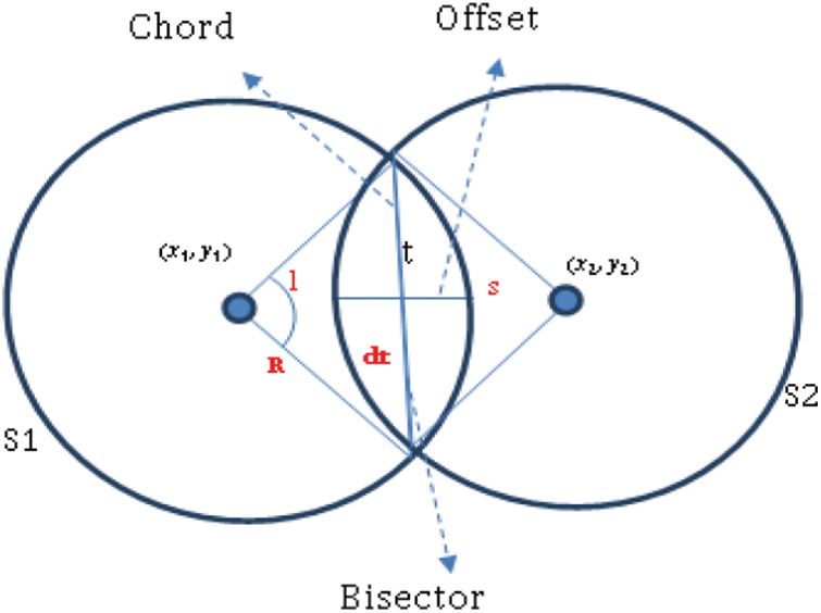
Figure 3: Offset calculation for node deployment
From dt, a bisector is drawn from s of S1 to s of S2, as the offset t. Based on the value of t, nodes can be arranged row and column-wise (see Fig. 4). To implement and make the DFWC as an efficient method, some of the assumptions are applied in the network and sensor nodes.
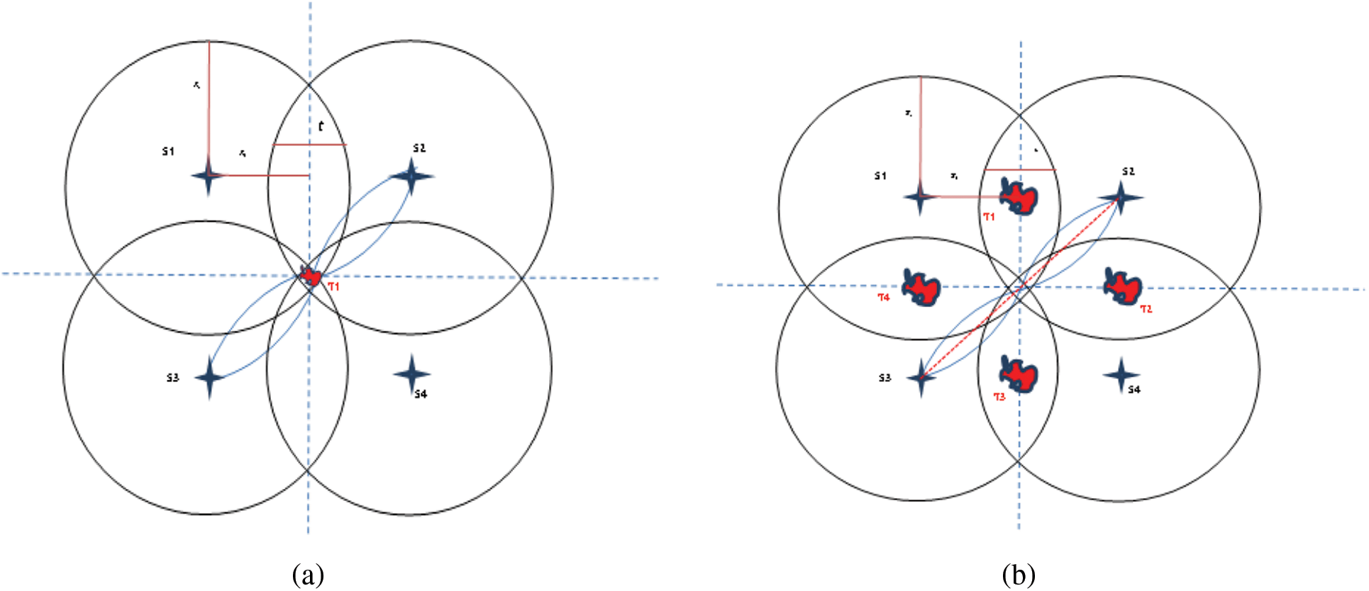
Figure 4: Target covered by sensors. (a) Single static target covered by static sensors, (b) Static multi-target covered by static sensors
In the first scenario SSTMSSN, target T1 is a static node, not moving anywhere, is monitored using four sensors as S1, S2, S3, and S4. Initially, N number of nodes is deployed randomly and distributedly in the network. After node distribution, the closest sensor nodes to the target nodes are adjusted for efficient target coverage. The target node T1 is deployed dynamically and randomly anywhere in the surveillance network. It is assumed that the surveillance network is a Wireless Sensor Network (WSN). In order to cover the target T1, η number of sensor nodes are deployed dynamically and randomly within the area where the target T1 is placed. Then move and adjust the locations of the sensor nodes to cover the target completely without high overlapping among the sensor nodes.
Fig. 4a illustrates the deployment scenario of the sensor nodes to cover the target T1. Sensor nodes are arranged in the form of rows and columns around the target. This arrangement is called as square model deployment. Let the nodes S1, S2, S3, S4 are the four nodes deployed in a square format where S1, S2 is placed in the first row and S2, S3 is placed in the second row, as:
The distance between T1 and the center of S1, S2, S3, and S4 are diagonally at equal distance. S1 is overlapping with S2 and S3. S2 is overlapping with S1 and S4 vice versa. The center point of the overlapping regions of the sensor node is perpendicular to the target node T1.
While node deployment Rs, Rtis verified based on the t value, arranged around the target (see Fig. 3). It is verified from the experiment of the deployment setup, two opposite nodes (S1, S4) or (S2, S3) can cover the target (T1) at a time. So, two nodes can be idle and save their energy at the maximum level. Based on the time duration (TD) assigned for target monitoring process nodes can be activated and idle. The energy consumption is calculated in accordance with (TD) from the currently activated nodes in the network.
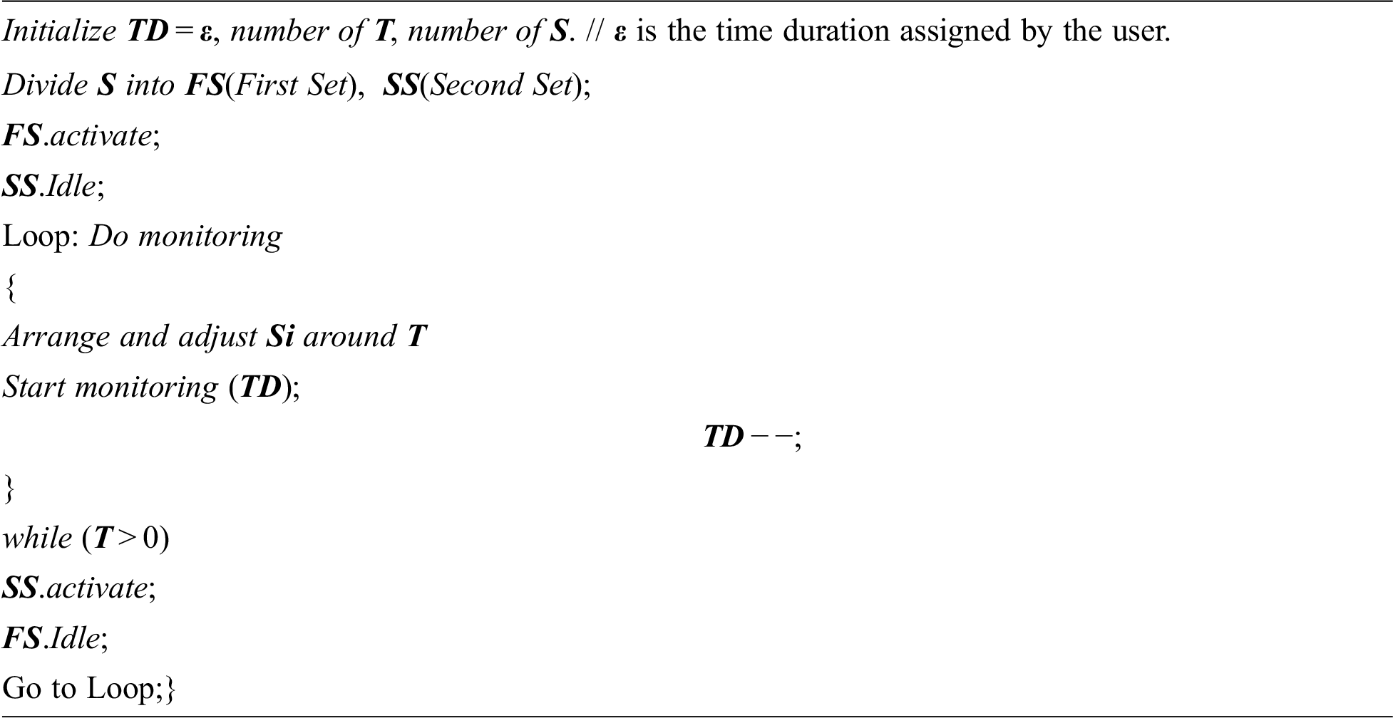
Once the time duration TD is over, then alternate nodes are activated as current nodes and other nodes have kept idle. Hence this SSTMSSN method proved as a better model for static target coverage with energy-efficient in WSN. Some of the real-time applications like building, shopping mall, and hospital monitoring are examples for SSTMSSN. The pseudo-code of the SSTMSSN model describes the set of sensor nodes are divided into two subsets as First Set (FS) and second subset (SS) for monitoring the target with energy efficiency. One round of operation is carried out in one TD, where FS is activated and SS is idealized. Means SS keeps its energy full, and FS consumes some amount of energy for target monitoring. Once TD becomes 0, then SS is activated and FS is idealized. This process is repeated until the process completed. The processing time is defined only by the application user or the application owner. It can be written as pseudocode and given below.
In the second scenario MSTMSSN, 1 to 5 number of target nodes can be monitored by four number of sensor nodes. The target nodes T1 to T5 are static and 4 sensors nodes S1, S2, S3, and S4 are arranged according to Fig. 4b. If the target node is placed within R of any sensor nodes, then it is very clear that those target nodes are covered accurately. If the target nodes are placed anywhere else, then the nodes are arranged for covering the target nodes.
In that case, T1 can be monitored by S1 and S2, T2 can be monitored by S2 and S4, T3 can be monitored by S4 and S3, and T4 can be monitored by S3 and S1. Target node T5 can be monitored by any sensors from S1 to S4, similar to SSTMSSN. Since two nodes can monitor a single target, it is easy to cover the target continuously with energy efficiency. Fig. 4a shows the overall area coverage in a network area and Fig. 4b shows the target area coverage. Scenario-1 and scenario-2 are also treated as an n-array model, where n = 4. A mathematical formula is derived for various targets and the associated number of sensor nodes can be used at the maximum. It helps to deploy the minimal number of sensors and activate the subset of sensors can be activated or idle during the target coverage process. By using Eqs. (9) and (10), the number of sensors used for target coverage is determined. For example, if the number of targets is 1, then the minimum number of sensors used for target monitoring is 4, where the number of nodes balancing the nodes is 2. In Tab. 1, the number of targets used in the network is changed from 1 to 6. For an increasing number of target nodes, the minimum number of sensor nodes is calculated and deployed using the Eqs. (9) and (10). Let n be the number of nodes. If the number of sensor nodes is 4n, then the number of sensor nodes used for energy balancing is
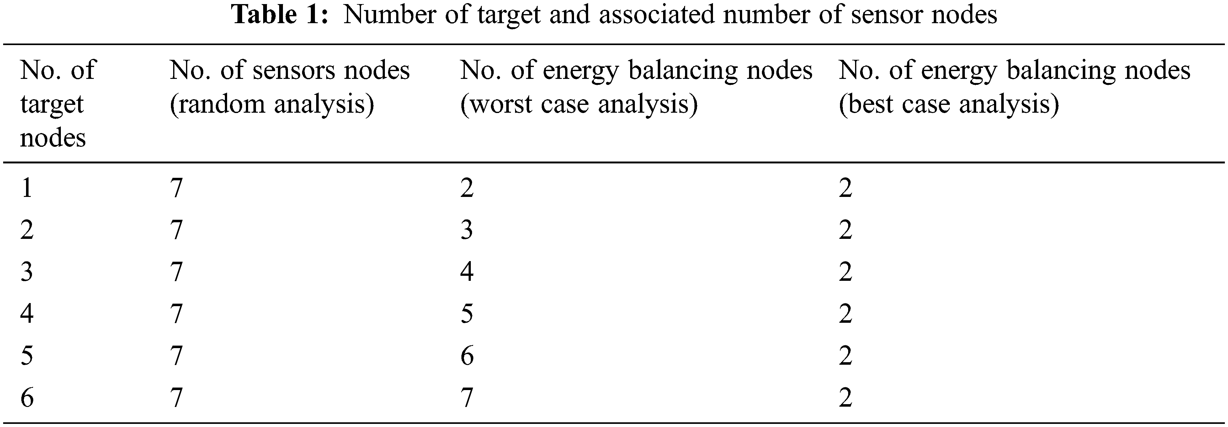
and if the number of sensor nodes is 2n, then the number of sensor nodes used for target coverage and energy balancing is
where the value of n can be determined by the application owner. This helps any new users who can decide about the number of sensor nodes used for target monitoring and it avoid wastage of time and cost.
In the scenario of SDTMDSN and MDTMDSN, the target and sensor nodes are dynamic nodes. The target nodes can move at any time any side in the network. Fig. 4 shows multiple (it may be single also) dynamic targets with multiple dynamic sensor nodes. Due to the dynamic nature of the target nodes, when the target node moves the sensor node also moves along with distance and velocity related to the linked target node. Also, the offset value in the overlapping area remains constant.
The final scenario illustrates how the dynamic nature of the target node can be monitored using sensor nodes. The paper assumed that the nodes are moving. So, as the target moves, with the same velocity and direction, the sensor nodes are also moving. The target moving directions and the sensor following directions are illustrated in Fig. 5. It is easy to identify that the target node can move in any direction. To maintain the velocity, moving the direction of the target node, the Particle Swarm Optimization (PSO) algorithm is used and updated to the sensor nodes.
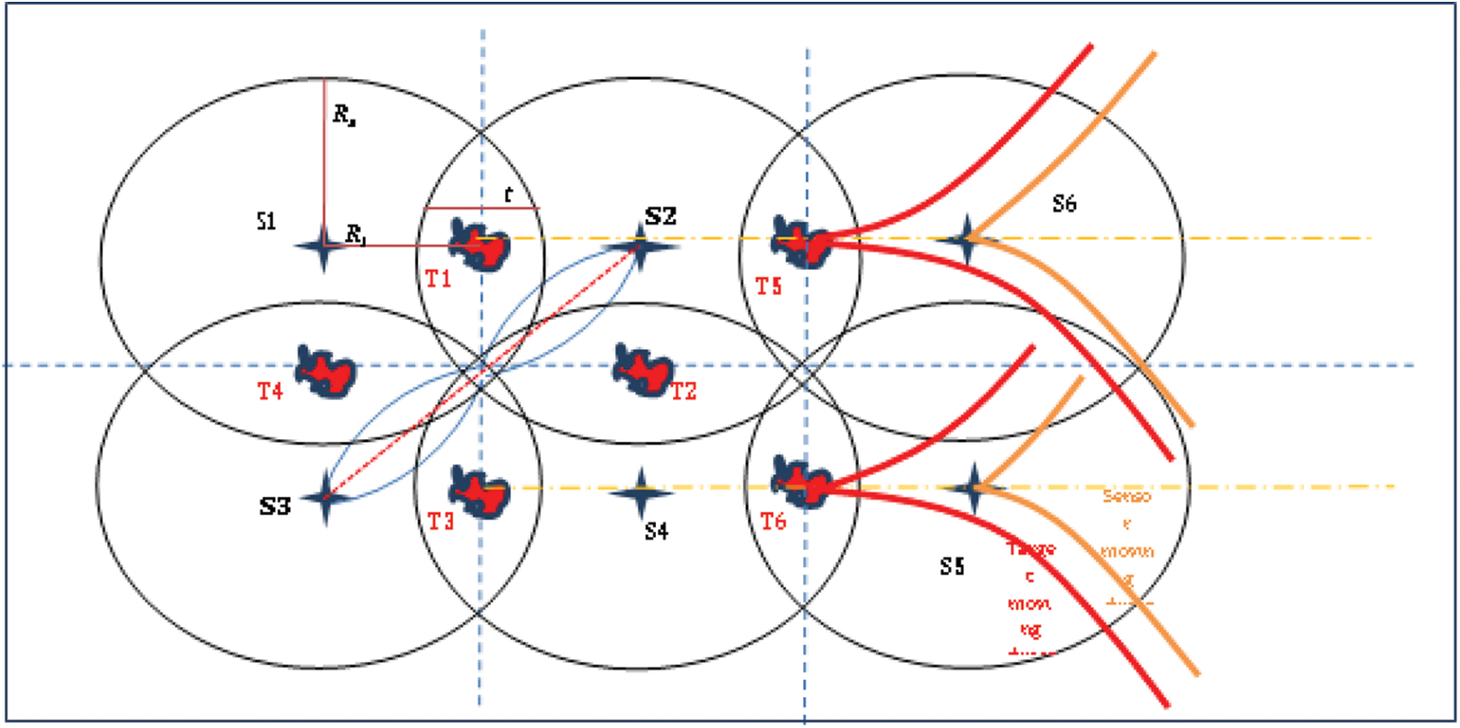
Figure 5: Single/Multiple dynamic target with multiple dynamic sensor nodes
One of the swarm intelligence algorithms that belong to Artificial Intelligence is Particle Swarm Optimization (PSO). AI techniques are used to simulate human behavior using computation methods. The set of all target nodes and sensor nodes information like node location, velocity and distance from the previous position to current positions are learned by the PSO from the routing table, maintained by the network routing protocol. PSO initializes the location of each node in the network (search space). The set of all sensor nodes are divided into various disjoint sets. Compute the distance and offset the value of the sensor nodes related to the target node. Assign the subset of the sensor nodes are particle group in a specific region. Compute the offset as the fitness value. If the location of the target node changes, then PSO will move the sensor nodes according to the target based on the distance and the offset value. Read the routing table at every interval of time. Calculate the variations in the target node and arrange the sensor nodes accordingly. In the case of target moving scenarios, the PSO algorithm is enabled for location updating to keep track of the target.
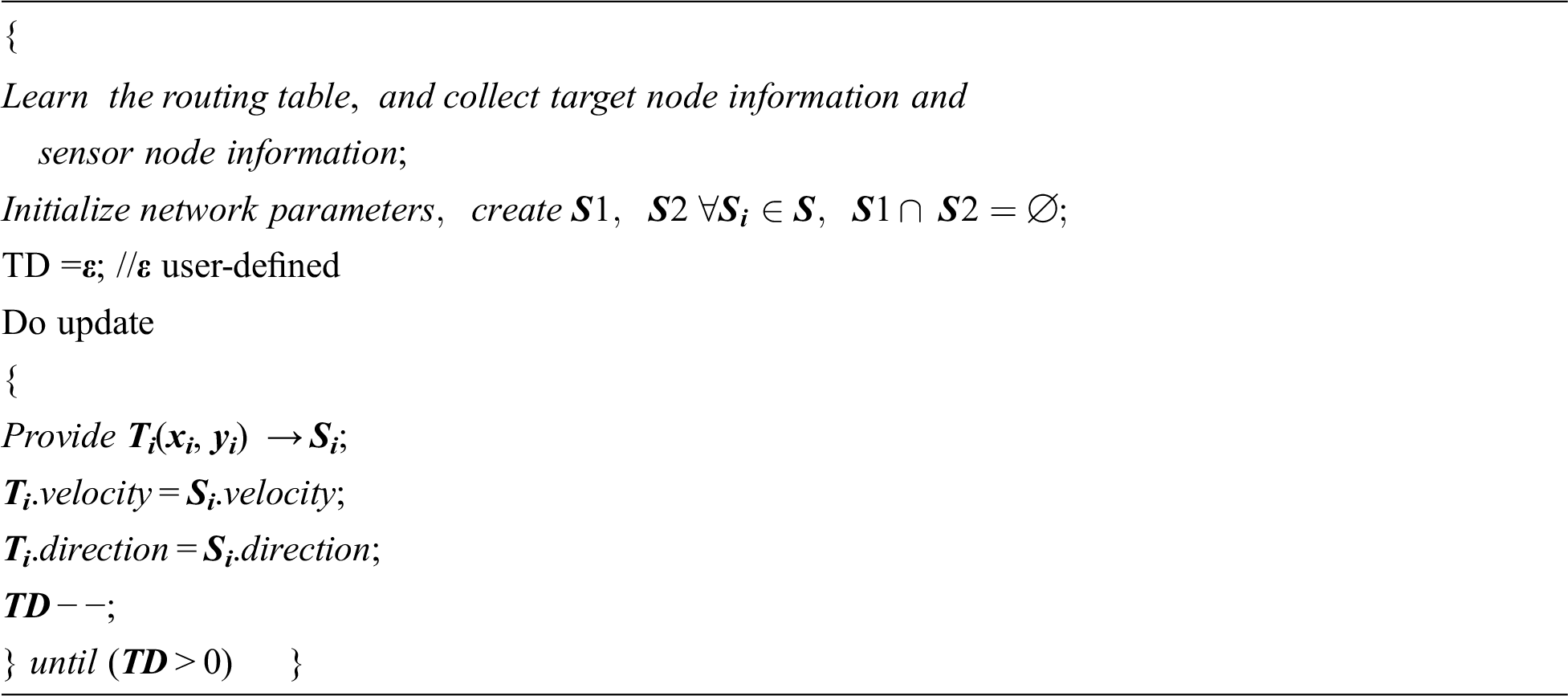
At each iteration of the process, the PSO algorithm learns the routing table and updates the information such as the location of target, direction, and velocity. The information obtained by the PSO is broadcasted to the sensor nodes who are in activate-mode. Once the sensor nodes collect the target information, it automatically calculates the distance and offset and other information to move accordingly. PSO algorithm obtains the target node ID, the ID of the sensors currently available in the active mode. Then only the network nodes can understand the target and the sensors need to be activated. The four models of the node deployment process to do an accurate target coverage problem are given in the following Pseudocode. The pseudo-code involves setting the network, initializing the network parameters, enabling the deployment models based on the dynamic behavior of the target nodes. According to the target nodes’ behavior, the sensor nodes can be activated. The programming model of the four different scenarios can call the PSO when the target node’s behavior is moving. During the coverage problem, the sensors decide themselves go to an active state or idle state. In the beginning, all the sensor nodes are in the active state, after adjustment only a subset of the sensor nodes is assigned into an idle state. According to the implementation, the computational complexity is also calculated for the target coverage problem which only depends on the density of the target and sensor nodes deployed in the network, which is O(n).
5 Simulation Results and Discussion
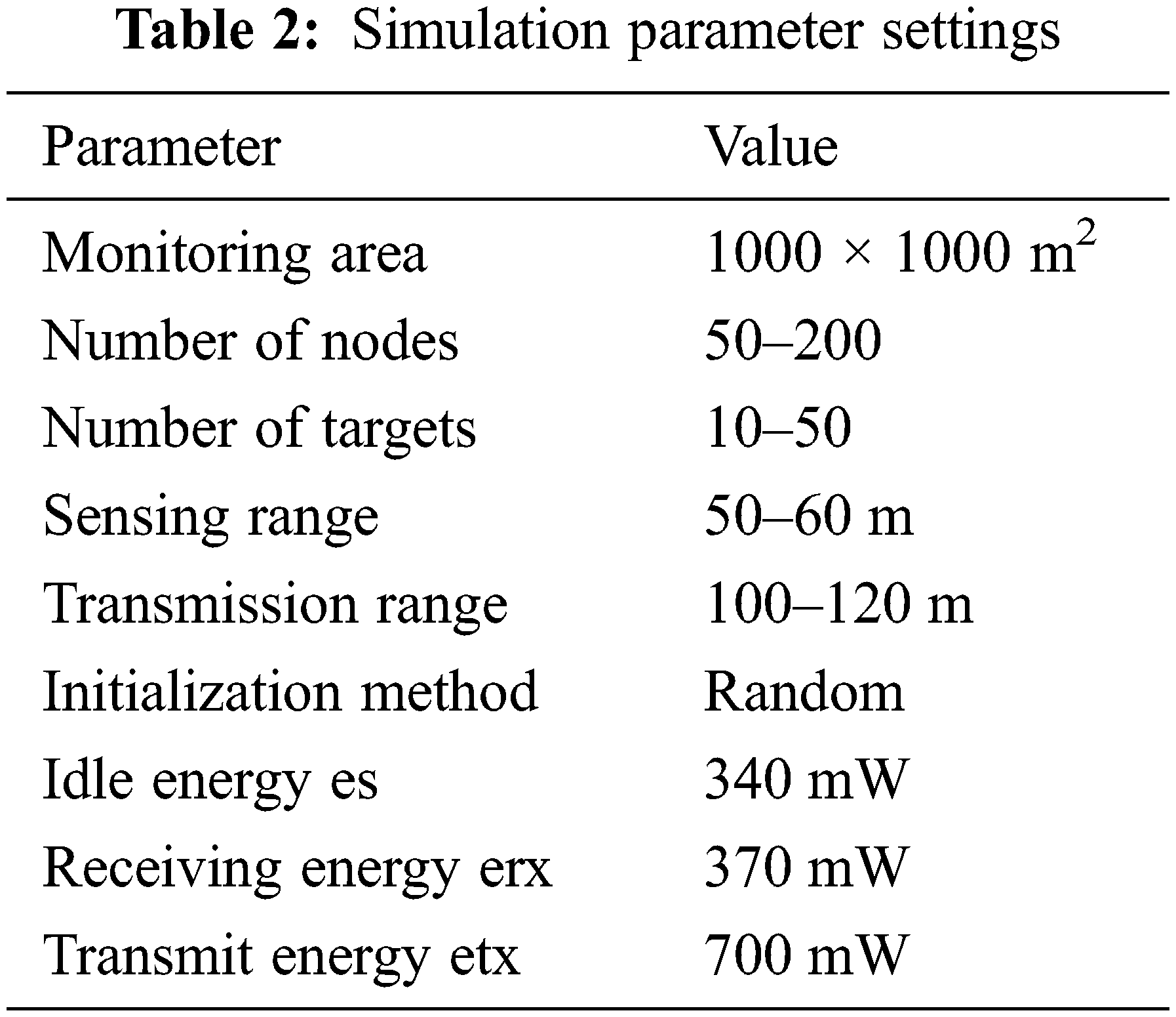
The suggested DFWC model is implemented and the results are confirmed using MATLAB software, as indicated in Fig. 1 and all the simulation parameters are listed in Tab. 2. A 1000 × 1000 network model is created in the MATLAB software and the nodes are created dynamically using graphics methods available in the software. Since MATLAB is scientific simulation software, which has a greater number of in-built tools and commands for creating user required model, can be animated. Based on the sensing model, the sensor node’s behavior is assigned, and all the sensor nodes are the same. For example, target can range from 10 to 50, and sensor node depends on the number of target (50 to 200). Each node’s starting battery level is set to 100 Joules. 380 mW of energy is utilized for sensing, calculating, processing, and controlling. Tx energy is 700 mW, Rx energy is 370 mW, and idle energy is 340 mW. The sensors’ detecting R-values range from 50 to 60 m, while their communication R-values range from 100 to 120 m. The experiment is carried out in a series of rounds. Each round of action includes two stages: startup and processing
Based on the first experiment, connected subsets are constructed for a variable number of targets using a variable number of sensor nodes distributed in the network. Based on the number of targets, the number of sensor nodes required to generate the coverage sets is computed and confirmed in the experiment. The calculation of the number of cover sets obtained from the experiment before and after the deployment of the DFWC is shown in Fig. 6 for self-assessment. As a result, the number of defined cover sets increases as the number of target nodes increases. When compared to the implementation before and after DFWC, the number of coverage sets is large yet inaccurate. The number of coverage sets created in the experiment is reduced and more accurate when DFWC is used. The number of coverage sets is proportional to the number of target nodes deployed in the network. The target coverage problem is efficient because the suggested DFWC algorithm creates fewer coverage sets in the network. DFWC utilized almost half of the nodes for target coverage, which is quite efficient when compared to other techniques shown in the literature study.
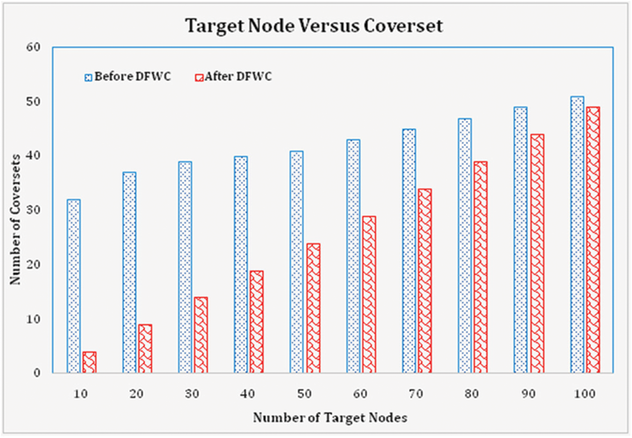
Figure 6: No. of target node vs. cover sets
Similarly, the number of cover sets from the installed sensor nodes is estimated from the experiment, and the result is shown in Fig. 7. The number of sensors utilized in the cover set is determined by computing the number of adjacent sensor nodes closest to the number of targets. It is calculated before and after the DFWC algorithm is deployed in the network for performance comparison reasons. The number of coverage sets acquired in a normal network is quite low; however the number of coverage sets obtained with DWFC is very high. The number of cover sets increases in direct proportion to the number of sensors. When compared to the other approaches, DFWC obtained 47 percent more coverage sets (without DFWC). The number of cover-sets in the network is proportional to the number of sensors deployed.
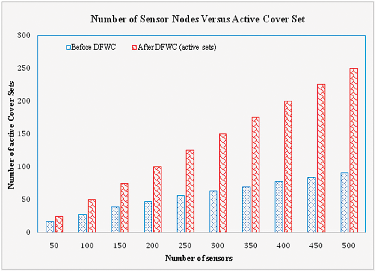
Figure 7: No. of sensor nodes vs. cover sets
Despite the fact that cover sets are developed and obtained, not all of them are used for target coverage or concurrent weather monitoring. To save energy, the cover set is divided into two parts: active and inactive. The active set is used for target coverage, while the rest of the nodes are inactive. Nodes in the active state will use a set amount of energy.
Another factor influencing the efficiency and performance of the suggested solution is its time complexity. Time complexity is computed by adding the time required to build and run a set of processes by the number of targets. Fig. 8 depicts the experimental results over time. It indicates that the amount of time required is proportional to the number of targets. As the number of targets rises, so does the time required for compilation and execution. The experiment, like time efficiency, calculates the power consumption of a major factor, and the corresponding result is presented in Fig. 9. The process in which the nodes are involved, such as data collection, transmission, and reception, determines the total energy consumed. It is also affected by the size of the data as well as the processing time. As a result, energy usage increases in direct proportion to node activity. If the target nodes are static, for example, power consumption is minimal; if the target nodes are dynamic, power consumption is high. Because the third and fourth scenarios involve moving targets, the power consumption for the first two scenarios is lower than the energy usage for the third and fourth scenarios.
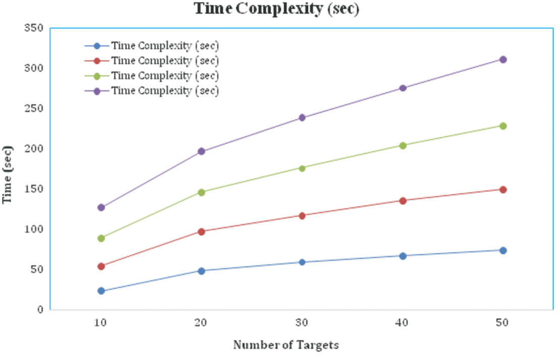
Figure 8: Time complexity comparison
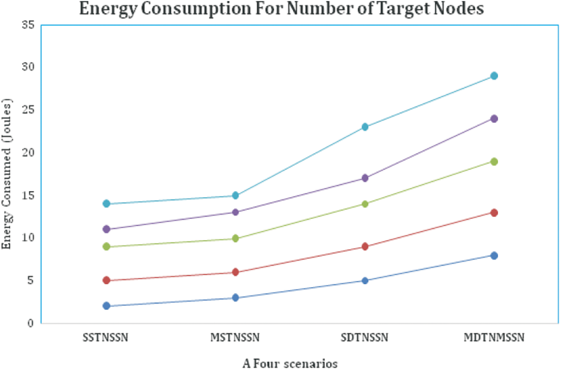
Figure 9: Energy calculation for target nodes
The power consumption of the sensor nodes is also calculated for performance verification. The energy is deducted from the total energy remaining in the sensor nodes based on node activity. Fig. 10 depicts the outcome of the relevant experiment. It shows that the quantity of energy consumed is related to the number of network nodes deployed. As the number of nodes increases, so does the power usage. The localization of the PSO algorithm is critical in determining target coverage accuracy. The original position of nodes is confirmed and compared to location data received by PSO to verify accuracy. Based on the comparison, the accuracy value is shown in Fig. 11.
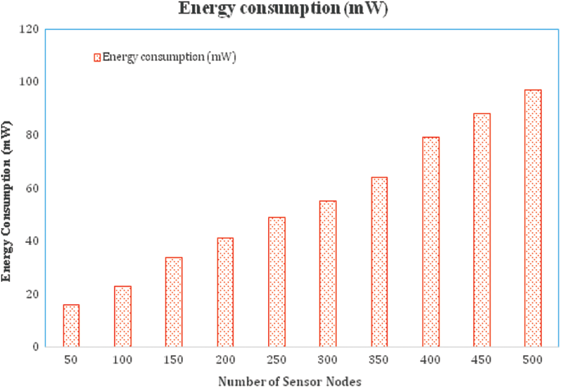
Figure 10: Energy calculation for sensor nodes
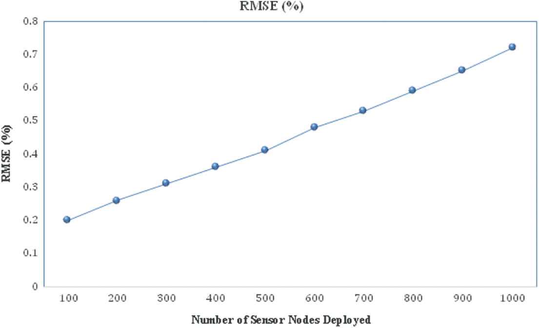
Figure 11: Localization error accuracy
Fig. 12 depicts the algorithm’s performance in increasing the size of the terrain. The geographical monitoring area ranges from 50 to 175 m and is comprised of 100 sensors and 20 targets. The density of sensor nodes is decreasing while the communication distance is increasing. Apart from the problems already mentioned, it has an effect on network stability and dependability, resulting in a loss of throughput and an increase in communication overhead. Based on the severe negative consequences, we can conclude that our technique is sensitive to changes in terrain size.
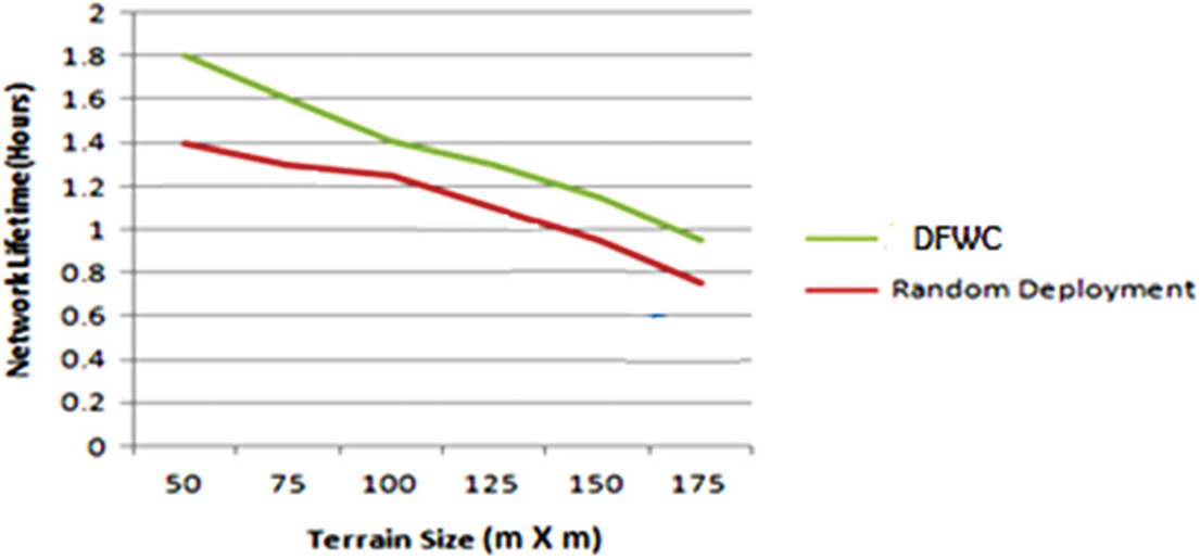
Figure 12: Network lifetime vs. Terrain size
The main objective of this paper is to design and implement a novel algorithm for efficient target coverage problems with energy efficiency. To increase the target coverage efficiency, a Dynamic Flexible Wheel Chain model is proposed, where it interconnects the coverage nodes in a chain, without any break, but the nodes are alternatively changed from the active state into an idle state. The proposed model is implemented in and experimented over four scenarios where the target nodes are considered as static and dynamic. From the experiment, it is obtained that the DFWC uses very a smaller number of active nodes for target coverage and saves the energy, it leads to provide increased network lifetime. Regarding time complexity the DFWC has taken only less amount of computational time than the other conventional approaches. By comparing all the results, it is concluded that the proposed DFWC model is highly suitable for accurate target coverage in WSN applications with improved energy. The simulation indicated that the DFWC approach outperforms random deployment in terms of target coverage. Furthermore, comparing an Omni directional and Directional Sensors model with different types of networks and sizes could be an extension of the work presented in this research.
Funding Statement: The authors received no specific funding for this research work.
Conflicts of Interest: The authors declare that they have no conflicts of interest to report regarding the current research work.
1. D. Agrawal and Q. A. Zeng, “Introduction to wireless and mobile systems,” in Global Engineering: Christopher M. Shortt, Cengage Learning 200 First Stamford Place, Suite 400 Stamford, CT 06902 USA, 3rd ed., pp. 1–610, 2011. [Google Scholar]
2. A. Kumar, V. Sharma and D. Prasad, “SDRS: Split detection and reconfiguration scheme for quick healing of wireless sensor networks,” International Journal of Advanced Computing, vol. 46, no. 3, pp. 1252–1260, 2013. [Google Scholar]
3. I. F. Akyildiz, W. Su, Y. Sankarasubramaniam and E. Cayirci, “Wireless sensor networks: A survey,” Computer Network, vol. 38, no. 4, pp. 393–422, 2002. [Google Scholar]
4. A. Mainwaring, D. Culler, J. Polastre, R. Szewczyk and J. Anderson, “Wireless sensor networks for habitat monitoring,” in Proc. of the 1st ACM Int. Workshop on Wireless Sensor Networks and Applications, Atlanta, GA, USA, pp. 88–97, 2002. [Google Scholar]
5. H. Liu, P. Wan, C. Yi, X. Jia, S. Makki et al., “Maximal lifetime scheduling in sensor surveillance networks,” in Proceedings IEEE 24th Annual Joint Conf. of the IEEE Computer and Communications Society, INFOCOM, Miami, FL, USA, pp. 2482–2491, 2005. https://doi.org/10.1109/INFCOM.2005.1498533. [Google Scholar]
6. A. Goldsmith and S. Wicker, “Design challenges for energy-constrained ad hoc wireless networks,” IEEE Wireless Communication, vol. 9, no. 4, pp. 8–27, 2002. [Google Scholar]
7. M. V. Ramesh, “Design, development and deployment of wireless sensor network for detection of landslides,” Ad Hoc Networks, vol. 13, pp. 2–18, 2014. [Google Scholar]
8. C. F. Hsin and M. Liu, “Network coverage using low duty-cycled sensors: Random & coordinated sleep algorithms,” in IPSN '04: Proc. of the 3rd Int. Symp. on Information Processing in Sensor Networks. ACM, New York, NY, USA, pp. 433–442, 2004. https://doi.org/10.1145/984622.984685. [Google Scholar]
9. A. Hatcher, “Algebraic Topology,” Cambridhe University Press, http://www.math.cornell.edu/˜hatcher, Ithaca, New York, pp. 1–560, 2001. [Google Scholar]
10. C. F. Huang and Y. C. Tseng, “The coverage problem in a wireless sensor network,” Mobile Network Applications, vol. 10, pp. 519–528, 2005. https://doi.org/10.1007/s11036-005-1564-y. [Google Scholar]
11. Y. Wang, X. Wang, D. Agrawal and A. Minai, “Impact of heterogeneity on coverage and broadcast reachability in wireless sensor networks,” in Proc. of the 15th Int. Conf. on Computer Communications and Networks, Arlington, pp. 63–67, 2006. https://doi.org/10.1109/ICCCN.2006.286246. [Google Scholar]
12. L. Lazos and R. Poovendran, “Stochastic coverage in heterogeneous sensor networks,” ACM Transactions on Sensor Network, vol. 2, no. 3, pp. 325–358, 2006. [Google Scholar]
13. K. Lin, X. Wang, L. Peng and X. Zhu, “Energy-efficient K-cover problem in hybrid sensor networks,” The Computer Journal, vol. 56, no. 8, pp. 957–967, 2013. [Google Scholar]
14. Q. Zhao and M. Gurusamy, “Lifetime maximization for connected target coverage in wireless sensor networks,” IEEE/ACM Transactions on Network, vol. 16, no. 6, pp. 1378–1391, 2008. [Google Scholar]
15. X. Deng, J. Yu, D. Yu and C. Chen, “Transforming area coverage to target coverage to maintain coverage and connectivity for wireless sensor networks,” International Journal of Distributed Sensor Networks, vol. 8, no. 10, pp. 1–12, 2012. [Google Scholar]
16. P. Leela Rani and G. A. Sathish Kumar, “Detecting anonymous target and predicting target trajectories in wireless sensor networks,” Symmetry, vol. 13, no. 4, pp. 1–22, 2021. [Google Scholar]
17. K. Subramanian and S. Shanmugavel, “A complete continuous target coverage model for emerging applications of wireless sensor network using termite flies optimization algorithm,” Wireless Personal Communications, 2021. https://link.springer.com/article/10.1007/s11277-021-08700-z. [Google Scholar]
18. L. I. Zhong, “Construction of node deployment model for wireless sensor network based on fuzzy data fusion,” in Journal of Physics: Conference Series, vol. 2044, (2021) 012133, no. 1, pp. 1–9, 2021. [Google Scholar]
19. C. Shao, “Wireless sensor network target localization algorithm based on Two-and three-dimensional delaunay partitions,” Journal of Sensors, 2021. https://doi.org/10.1155/2021/4047684. [Google Scholar]
20. N. Cao, S. Choi, E. Masazade and P. K. Varshney, “Sensor selection for target tracking in wireless sensor networks with uncertainty,” IEEE Transactions on Signal Processing, vol. 64, no. 20, pp. 5191–5204, 2016. [Google Scholar]
21. M. Anvaripour, M. Saif and M. Ahmadi, “A novel approach to reliable sensor selection and target tracking in sensor networks,” IEEE Transactions on Industrial Informatics, vol. 16, no. 1, pp. 171–182, 2019. [Google Scholar]
 | This work is licensed under a Creative Commons Attribution 4.0 International License, which permits unrestricted use, distribution, and reproduction in any medium, provided the original work is properly cited. |