DOI:10.32604/iasc.2023.026799
| Intelligent Automation & Soft Computing DOI:10.32604/iasc.2023.026799 | |
| Article |
Hybrid Deep Learning Based Attack Detection for Imbalanced Data Classification
1Department of Computer Science, Faculty of Computing and Information Technology, King Abdulaziz University, Jeddah, Saudi Arabia
2Department of Computer Science, Faculty of Computer Science and Engineering, University of Hail, Hail, Saudi Arabia
*Corresponding Author: Rasha Almarshdi. Email: rabdullahalmarshdi@stu.kau.edu.sa
Received: 04 January 2022; Accepted: 23 February 2022
Abstract: Internet of Things (IoT) is the most widespread and fastest growing technology today. Due to the increasing of IoT devices connected to the Internet, the IoT is the most technology under security attacks. The IoT devices are not designed with security because they are resource constrained devices. Therefore, having an accurate IoT security system to detect security attacks is challenging. Intrusion Detection Systems (IDSs) using machine learning and deep learning techniques can detect security attacks accurately. This paper develops an IDS architecture based on Convolutional Neural Network (CNN) and Long Short-Term Memory (LSTM) deep learning algorithms. We implement our model on the UNSW-NB15 dataset which is a new network intrusion dataset that categorizes the network traffic into normal and attacks traffic. In this work, interpolation data preprocessing is used to compute the missing values. Also, the imbalanced data problem is solved using a synthetic data generation method. Extensive experiments have been implemented to compare the performance results of the proposed model (CNN+LSTM) with a basic model (CNN only) using both balanced and imbalanced dataset. Also, with some state-of-the-art machine learning classifiers (Decision Tree (DT) and Random Forest (RF)) using both balanced and imbalanced dataset. The results proved the impact of the balancing technique. The proposed hybrid model with the balance technique can classify the traffic into normal class and attack class with reasonable accuracy (92.10%) compared with the basic CNN model (89.90%) and the machine learning (DT 88.57% and RF 90.85%) models. Moreover, comparing the proposed model results with the most related works shows that the proposed model gives good results compared with the related works that used the balance techniques.
Keywords: IoT; IDS; deep learning; machine learning; CNN; LSTM
In recent years, Internet of Things (IoT) has become one of the most important technologies. IoT is defined as a set of technologies that make a wide range of devices and objects connect and interact with each other via machine-to-machine (M2M) communications [1]. These devices are embedded with sensors and electronics connected with the internet to collect and exchange data [2]. There are many applications of IoT, including (transportation, infrastructure management, healthcare and medical monitoring, home automation, etc.) [3]. As shown in Fig. 1, the architecture of IoT is divided into four layers. The physical layer contains sensing devices to sense and remotely monitor any physical phenomenon in the real world. The network layer connects the sensors using access points such as Wi-Fi to the web service, datacenter, or cloud for data transmission. The support layer provides a platform for IoT applications to analyze, store, and handle transmitted data. The application layer includes user services and applications for IoT, which can be accessed via the application layer interface [4].
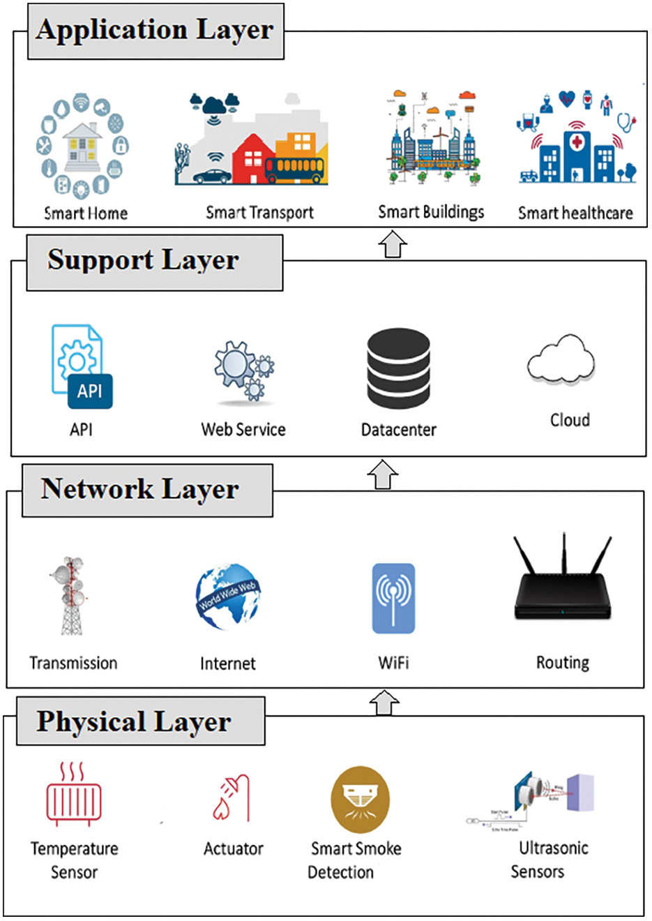
Figure 1: IoT architecture
The dramatic increase in data generation and transmission across heterogeneous and distributed infrastructure and resource constrained devices makes security very challenging [5]. The IoT is the most vulnerable to various types of attacks because of the spread of its gradual development of infrastructure without providing measures to defend against security attacks [6,7]. Intrusion Detection Systems (IDSs) are software applications used for network monitoring to detect malicious activity or policy violations [8]. There are two classes for IDS: signature-based and anomaly-based. Signature-based IDS uses specific signatures already known to it, making it effective for detecting known attacks, but it cannot detect newly introduced attacks. In contrast, anomaly-based IDS detects the unusual deviations by identifying the abnormal behavior pattern in traffic, where a statistical model is built to define normal behavior. Therefore, new attacks can be detected because that their statistical behavior differs from the behavior of normal traffic. However, it is practically useless because it suffers from high false alarm rates where not every anomaly is caused by an attack [9].
Many machine learning techniques have been proposed for IDS. These techniques rely on algorithms to learn directly from the data without explicitly programming, which is helpful considering the great diversity of the traffic [10]. However, despite these advantages, anomaly-based detection algorithms have a high false positive rate which is the main reason for the lack of adoption of machine learning based-anomaly IDS. Also, machine learning models learn the traffic of a dataset and not the traffic to be monitored [11]. Deep learning methods can learn the highly complex and nonlinear functions required to predict different types of abnormal behavior and thus can provide improved performance. Deep learning can automatically extract important features and capture deep learning relationships automatically from raw data without manually identifying features. This method can capture patterns of input data to produce a high detection rate [12].
Even though there are currently some proposed solutions to detect security attacks based on both machine learning and deep learning algorithms in IoT, most of these solutions did not consider the problem of imbalanced data. Imbalanced data is a classification problem that gives poor accuracy. This paper aims to develop an IDS based on a hybrid deep learning algorithm to detect IoT attacks on imbalanced datasets such as UNSW-NB15, a recent network intrusion dataset.
The paper objectives are given as follows.
• Develop an IDS based on a hybrid deep learning model that combines Convolutional Neural Network (CNN) and Long-Short Term Memory (LSTM) algorithms.
• Solve the imbalanced data problem in the UNSW-NB15 dataset using a synthetic data generation method.
• Validate the contribution of the proposed model by comparing its results with a basic CNN model using both a balance and imbalance dataset.
• Validate the contribution of the proposed model by comparing its results with benchmark machine learning models (Decision Tree (DT) and Random Forest (RF)) using both a balance and imbalance dataset.
The paper is organized as follows. Section 2 describes the literature review. The methodology of the work is described in Section 3. The experimental results and discussions of the proposed model performance are presented in Section 4. Finally, the conclusion and future work is described in Section 5.
Security of sensors and data collection and transmission over unsecured IoT networks is a critical issue. As shown in Fig. 2, various attacks may be directed to the IoT system, and these attacks can be categorized based on the IoT architecture layers [13]. The sensors are most vulnerable to physical attacks in the physical layer due to their widespread in IoT environments such as node tempering and fake node [14]. The network layer is characterized by having security measures, but it is not without some problems that may affect the confidentiality of data. The possible attacks on the network layer include Denial of Service (DoS) and Distributed Denial of Service (DDoS) [15]. The support layer provides powerful computing, data storage, brokers, machine learning, etc. Therefore, this layer must be protected from attacks and security breaches such as flooding in cloud, SQL injection, and signature wrapping [16]. Sharing data is one of the most characteristics in the application layer, so it faces data theft and privacy problems. The attacks on the application layer include data theft, DDoS, malicious X script, and reprogram attack [17].
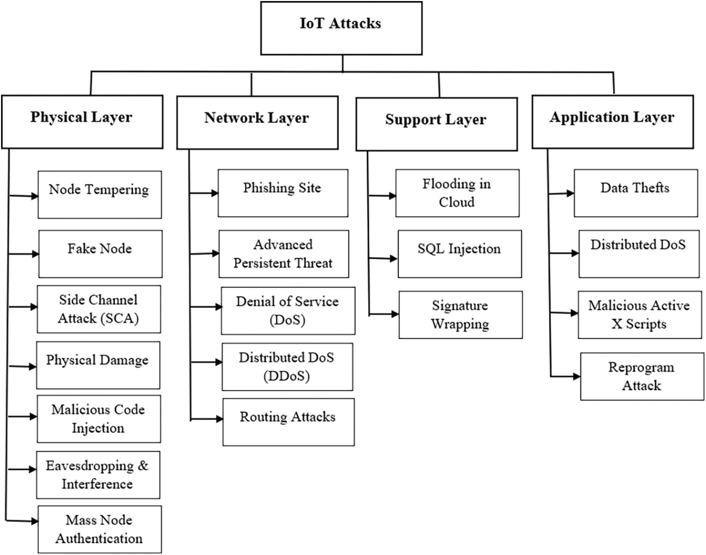
Figure 2: IoT security attacks
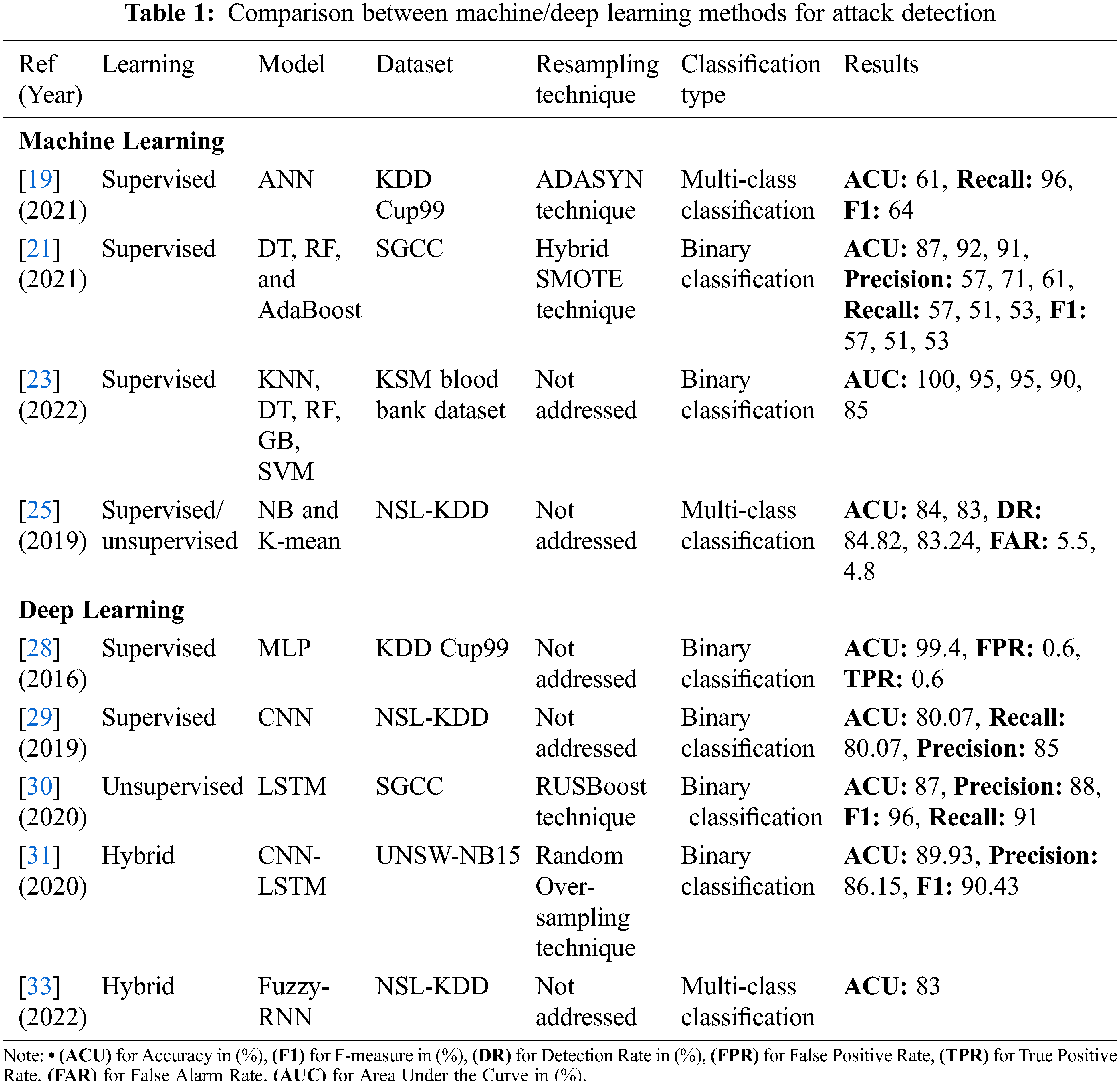
Few works have been proposed to manage the issue of imbalanced data to improve the performance of the classification. The following presents the most current studies that adopted machine learning and deep learning to detect security attacks in IoT networks.
2.1.1 Machine Learning Solutions
Machine learning improves the system’s ability to learn automatically and improve from experience without being explicitly programmed [18]. Two main categories in machine learning: supervised learning includes (Decision Tree (DT), Random Forest (RF), Naïve Bayes (NB), Artificial Neural Network (ANN), Logistic Regression (LR), Support Vector Machine (SVM), K-Nearest Neighbors (KNN)). Unsupervised learning includes (K-means and Hierarchical Clustering).
Bagui et al. [19] proposed an IDS based on the ANN model. The proposed model has been applied to the KDD Cup 99 dataset [20], which is a popular dataset used in intrusion detection. They solved the imbalanced data using an the Adaptive Synthetic Sampling (ADASYN) technique. The experiment indicates that if the dataset is completely imbalanced, the oversampling method increases recall substantially, while there is no high impact if the dataset is not completely imbalanced. The results achieved 61% accuracy, 96% recall, and 64% f-measure. Arif et al. [21] proposed a detection model on a State Grid Corporation of China (SGCC) dataset [22]. They solve the imbalanced data using a hybrid resampling technique named synthetic minority oversampling technique with a near miss. Three algorithms are used: DT, RF, and adaptive boosting (AdaBoost) to train the model. They used the Bayesian optimizer to simplify the tuning process of the algorithms. The results show that RF is better than DT and AdaBoost where it achieved 92% accuracy compared with DT 87% and AdaBoost 91%.
Shankar Komathi Maathavan et al. [23] employed different machine learning models to find the best classification to avoid data breaches in electronic healthcare data. They used a real dataset from the KSM blood bank [24]. The experiment is done based on two tests: two features and four feature analyses. For two feature analyses, the DT, RF, and Gradient Boosting (GB) classifiers outperform the SVM and KNN in terms of accuracy, 100%. For four feature analysis, the KNN outperforms the rest of the models. Pajouh et al. [25] proposed an IDS model based on two-layer dimension reduction and a two-tier classification module. The model uses factor evaluation and linear discriminate evaluation of dimension reduction module to spate the excessive dimensional dataset to a decreased one with lesser features. For two-tier classification, they used NB and K-mean. The model was applied to the NSL-KDD dataset [26] and improved the imbalanced dataset version of the KDD Cup 99 dataset. From the results, the NB achieved 84% accuracy, 84.82% detection rate, and 5.5 false alarm rate while, K-mean achieved 83% accuracy, 83.24% detection rate, and 4.8 false alarm rate.
Deep learning is a subset of machine learning known as a hierarchical learning technique because the algorithms are stacked in a hierarchical level of ANN to carry out the machine learning process. The ANN works like the human brain in its classification accuracy for complex tasks. Also, deep learning is classified into two main categories: supervised learning includes (Multi-Layer Perceptron (MLP), Convolutional Neural Network (CNN)) and unsupervised learning includes (Recurrent Neural Network (RNN), Auto-Encoder (AE), and Restricted Boltzmann Machine (RBM)) [27].
Hodo et al. [28] proposed an IDS based on the MLP algorithm. The attack source is from an external user and targets the server node only. They applied the experimental results on the KDD Cup 99 dataset, proving the effectiveness of the proposed system where it achieves 99% accuracy. Teyou et al. [29] built a CNN model to detect intrusions in the cyber-physical system. They used the NSL-KDD dataset, and the model’s performance is compared with the state of the art. The results give 80.07% accuracy, 80% recall, and 85% precision for binary classification. Adil et al. [30] proposed a detection model using the LSTM technique to detect normal and attack traffic in the power system. They implemented the model using the SGCC dataset. The imbalanced data was addressed using the under-sampling boosting (RUSBoost) technique. The proposed model achieved 87% accuracy, 96% f-measure, 88% precision, 91% recall, and 87% Area Under Curve (AUC).
Azizjon et al. [31] proposed IDS using a one-dimensional CNN combination with the LSTM model. They used the UNSW-NB15 dataset [32], a modern network intrusion dataset. The imbalanced dataset is solved using a random over-sampling technique. They compare the proposed model with 1D CNN, RF, and SVM. For the imbalanced dataset, the results show that the RF is outperformed the other models in terms of accuracy, where it achieved 87.82% while the proposed model achieved 85.11%, 1D CNN achieved 83.19%, and SVM achieved 68%. For the balanced dataset, the results show that the 1 D CNN with three layers is outperformed the other models in terms of accuracy where it achieved 91% while the proposed model achieved 89.93%, RF achieved 87.39%, and SVM achieved 61.69%. Praveen Ramalingam et al. [33] presented a hybrid IDS that combines fuzzy and RNN algorithms. This combination gives better classification and precision compared with machine learning classifiers. They implemented the proposed IDS on the NSL-KDD dataset. The imbalance data issue is not addressed in this work. The proposed IDS gives 83.94% accuracy, which is the highest compared with NB, RF, MLP, and SVM classifiers.
The literature indicates that the current solutions based on machine learning algorithms have shown reasonable results. However, they suffer from a high false positive rate. The solutions based on deep learning have proven their effectiveness to improve the detection rate, accuracy, and false positive rate. Deep learning can capture input data’s behavior due to its ability to extract complex patterns and learn from the huge data. Even though there are currently some proposed solutions to detect different types of attacks based on both machine learning and deep learning algorithms in IoT, most of the current solutions do not consider the problem of imbalanced data. Tab. 1 displays the comparison between machine learning and deep learning methods to detect security attacks in IoT.
In this work, an IDS is developed based on a hybrid deep learning model for security attacks detection in the IoT environment. Fig. 3 illustrates the flowchart of the IDS for network traffic classification using different techniques.
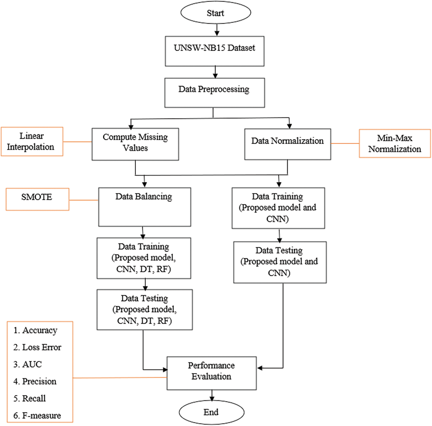
Figure 3: IDS flowchart
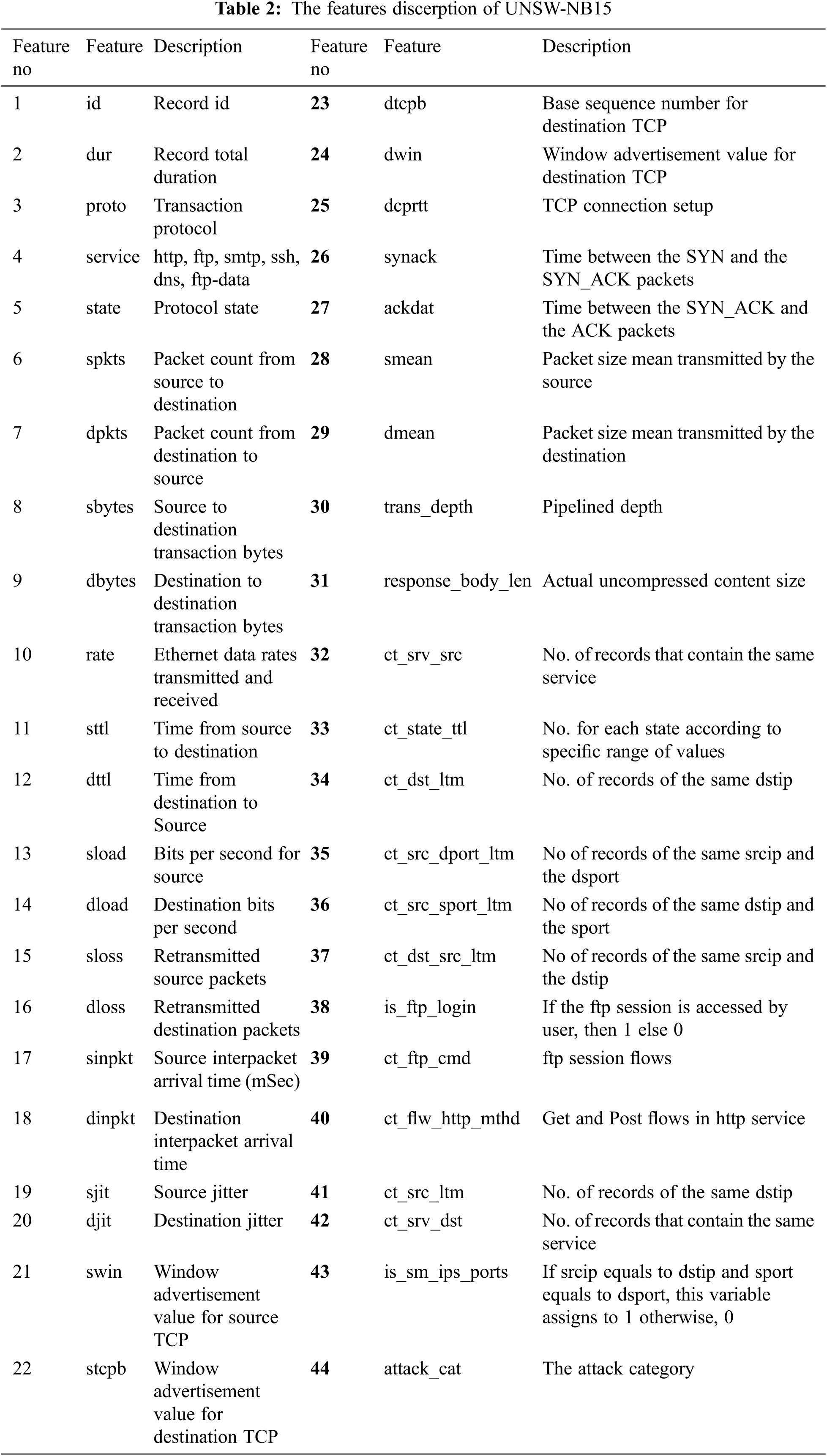
A new network intrusion dataset is selected named UNSW-NB15, where the network traffics and raw packets were monitored and recorded via the modern network infrastructure. The UNSW-NB15 was created using an IXIA PerfectStorm tool in the Cyber Range Lab of the Australian Centre for Cyber Security (ACCS) in 2015 [34]. There are nine security attacks in the UNSW-NB15, including Fuzzers, Analysis, Backdoor, DoS, Exploit, Generic, Reconnaissance, Shellcode, and Worm. The UNSW-NB15 contains 44 features without the class label, as shown in Tab. 2. The features include packet-based and flow-based features in different data types such as nominal, float, integer, and binary. The packet-based features assist the inspection of the payload with the headers of the packets. The flow-based features are based on a direction, inter-arrival time, and an inter-packet length. The dataset is labeled the normal flow to “0” and the attack flow to “1”. The dataset is partitioned into a training set with 175341 records (56000 for normal flow and 119341 for attack flow) and a testing set with 82332 records (37000 for normal flow and 45332 for attack flow).
In data preprocessing, we divide the task into two steps. First, compute the missing value using a linear interpolation method. Second, normalize the data using a Min-Max scaling method.
3.2.1 Computing the Missing Value
A real-time dataset always consists of many missing values, resulting from data failure or corruption during its recording, unreliable data transmission, and system maintenance and storage issues. The missing value is calculated using a linear interpolation method as
The
where
Normalization is a scaling method that converts all data features into a common scale. The minimum and maximum values range of the continuous feature in UNSW-NB 15 are significantly different. A Min-Max scaling method is used to facilitate the arithmetic processing, and the range of values of each feature is uniformly linearly mapped in the range 0 and 1. The Min-Max scaling method can be defined as
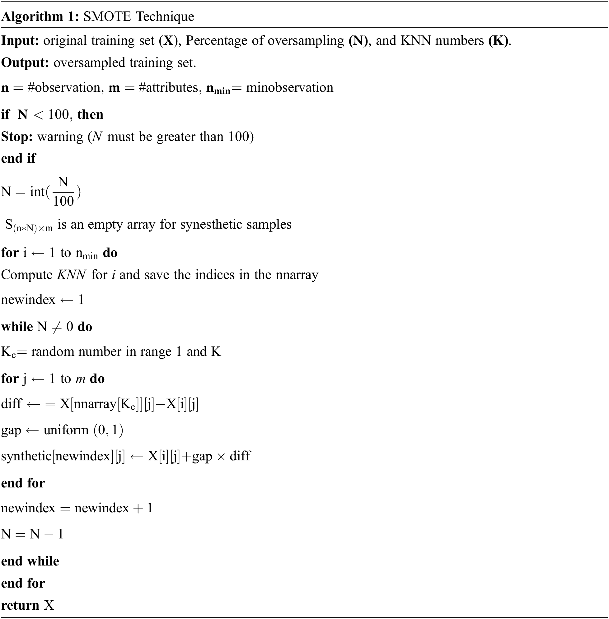
The UNSW-NB15 dataset is not perfectly balanced, where one class is lower than the other class. In the following figure, the x-axis represents the class (0 for normal and 1 for attack), and the y-axis represents the count of the class. In Fig. 4a, the distribution of classes shows that the normal class is lower than the attack class which caused a classification problem known as an imbalanced dataset which makes the model biased to the direction of the majority. The imbalanced dataset problem can be handled based on two approaches: a cost function-based approach or a sampling-based approach. In this paper, we chose the sampling-based approach. There are two types of sampling-based approaches: an under-sampling and an over-sampling approach for disparity reducing between two classes. The under-sampling technique reduces the size of the dataset by randomly selecting the examples from the majority class and deleting them from the dataset. This random deletion may cause important data to be deleted, resulting in less accuracy [35]. The over-sampling technique randomly duplicates examples in the minority class. Although this technique does not cause data loss, it may be subject to overfitting due to the redundancy of data points. This paper uses a Synthetic Minority Over-sampling Technique (SMOTE) to avoid the overfitting problem. SMOTE is an over-sampling technique that allows the generation of synthetic samples for the minority categories. The idea of SMOTE depends on the KNN algorithm, where it takes a sample from a dataset and considers its nearest neighbors in the feature space [36]. If
where
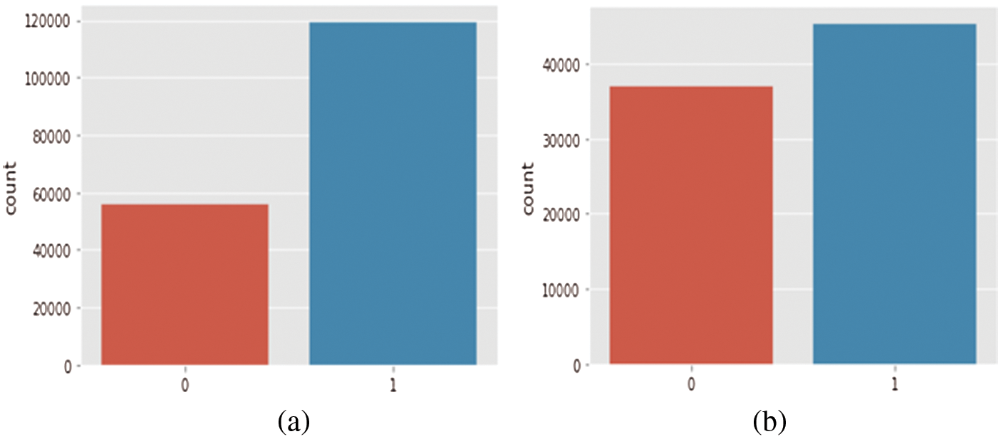
Figure 4: Data distribution (a) before SMOTE (b) after SMOTE in UNSW-NB15
The proposed IDS is based on a hybrid deep learning model which combines the Convolutional Neural Network (CNN) and Long Short-Term Memory (LSTM) algorithms. This aggregation combines their feature extraction, memory retention, and classification abilities, giving better accuracy than the single models. As shown in Fig. 5, the proposed model architecture consists of three layers: CNN, LSTM, and dense layers.
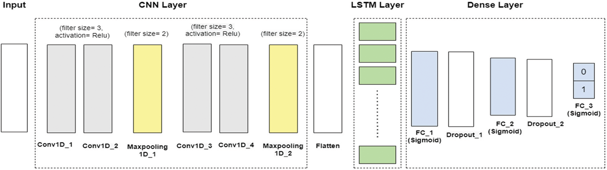
Figure 5: Proposed model architecture
3.4.1 Convolutional Neural Network Layer
CNN is designed to detect objects, and it can detect unknown attacks. CNN extracts features automatically and performs a difficult operation on hidden layers to minimize the sharing of the parameters and weights. CNN contains multiple convolutional layers, pooling layers, and fully connected layers [37]. The architecture of our CNN layer consists of four convolutional (Conv) layers. Each group of two convolutional layers is followed by one pooling layer. The input features are formed into a 1D matrix with 44 input features. Conv 1 and Conv 2 operated with (convolution filters = 32, filter size = 3, and output shape = 32 × 64 feature matrix). Conv 3 and Conv 4 operated with (convolution filters =64, filter size = 3, and output shape = 16 × 128 feature matrix). Each filter generates an activation map with padding value 1. The Relu (Rectified Linear Unit) activation function is used in the convolution layers. It is defined as
where
The pooling layer is another building block of CNN. It minimizes the dimensionality of the features map and thus minimizes overfitting and training time. There are two common pooling methods, which are average-pooling and max-pooling. Max-pooling has been utilized in this model. It calculates the maximum value in each feature map. The output of convolutions is directed to the max-pooling layer. We use two max-pooling layers with (pooling size = 2 and stride = 1). The formula of the max-pooling layer is calculated as
where
3.4.2 Long Short-Term Memory Layer
Long Short-Term Memory (LSTM) is a special type of RNN designed to solve the short-term memory problem of RNN, where it aims to handle time-series data. The hybrid CNN+LSTM model combines both convolutional layers to extract features and LSTM units for sequence prediction supporting across time. The output of CNN is directed into LSTM units to model the signal in time and train the weights. The LSTM units consist of three gates: forget, input, and output gates. These gates control how the information in a data sequence comes, stores in, and leaves the network. The first step is to determine whether the previous information from the previous timestamp should be kept or forgotten. The forget gate takes the output value of the last timestamp and the input value of the current timestamp to generate output between 0 and 1. The output of the forget gate is calculated as
where
Now, the forget gate determines what information is added in the cell state. It takes the last output and input values at the current timestamp to the input gate. Then, it calculates it to obtain the output value and the candidate cell state of the input gate. The output is calculated as
where
where
Then, the output gate accepts the output and input as the input value at timestamp t and obtains the output of the output gate. The final output value is obtained by calculating the output of the outputs and the state of the cell. The final output is calculated as
where
The output in the dense layer is directed when the LSTM units model the signal to learn higher-order feature representations suitable for separating the output into two classes: normal and attack. At the end of the architecture, we add three fully connected (FC) layers and two dropout layers. The FC layer is added with the sigmoid function, which is used for classification based on low-level features after the LSTM units. The sigmoid activation is described as
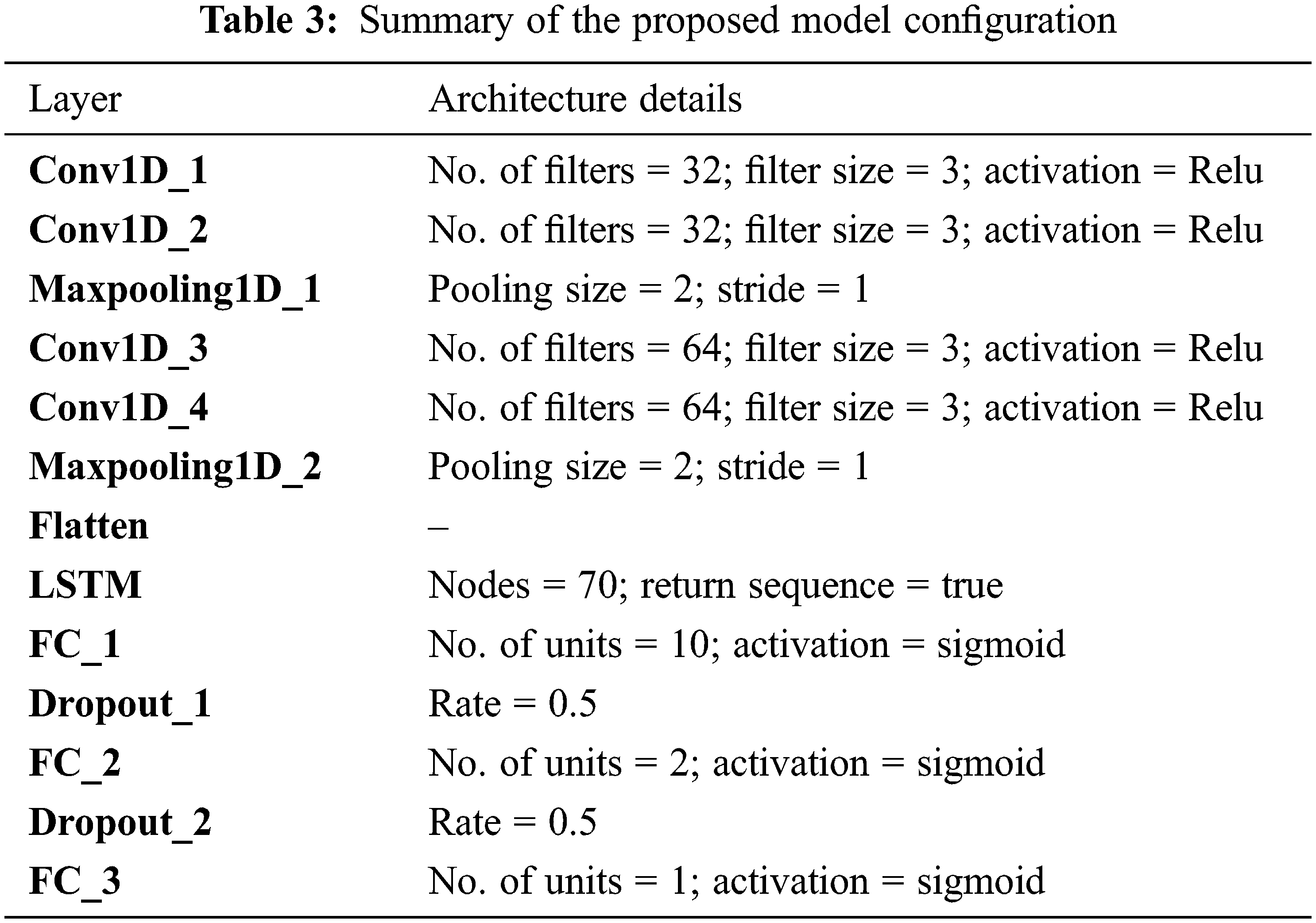
The dropout regularization method is used after the first and second FC layers to avoid the overfitting problem during the training. Tab. 3 describes the summary of the proposed model configuration.
The time complexity is applied to training time and testing time. Only convolutional layers are included in the computation where pooling, LSTM, and FC layers always take 10% to 15% computational time. The time complexity of the proposed model can be calculated as
where
4 Experiments and Results Discussion
In this section, First, describes the settings of the experiments. Next, it presents the performance matrices that are used to evaluate the performance of the model. Finally, it provides performance comparison under different experimental scenarios.
The proposed model uses Python 3.6 with two deep learning libraries such as TensorFlow 1.15 and Keras libraries. The experiments environment that is used to develop the model is Jupyter Notebook. In addition, various libraries are used, such as Pandas for data analysis, NumPy to support the multi-dimensional array and matrix data structures, and Matplotlib for data visualization and graphical plotting. There is a relationship between the size of the dataset and the model performance, where more data results in better performance. The dataset size is chosen to be 80% for training and 20% for testing.
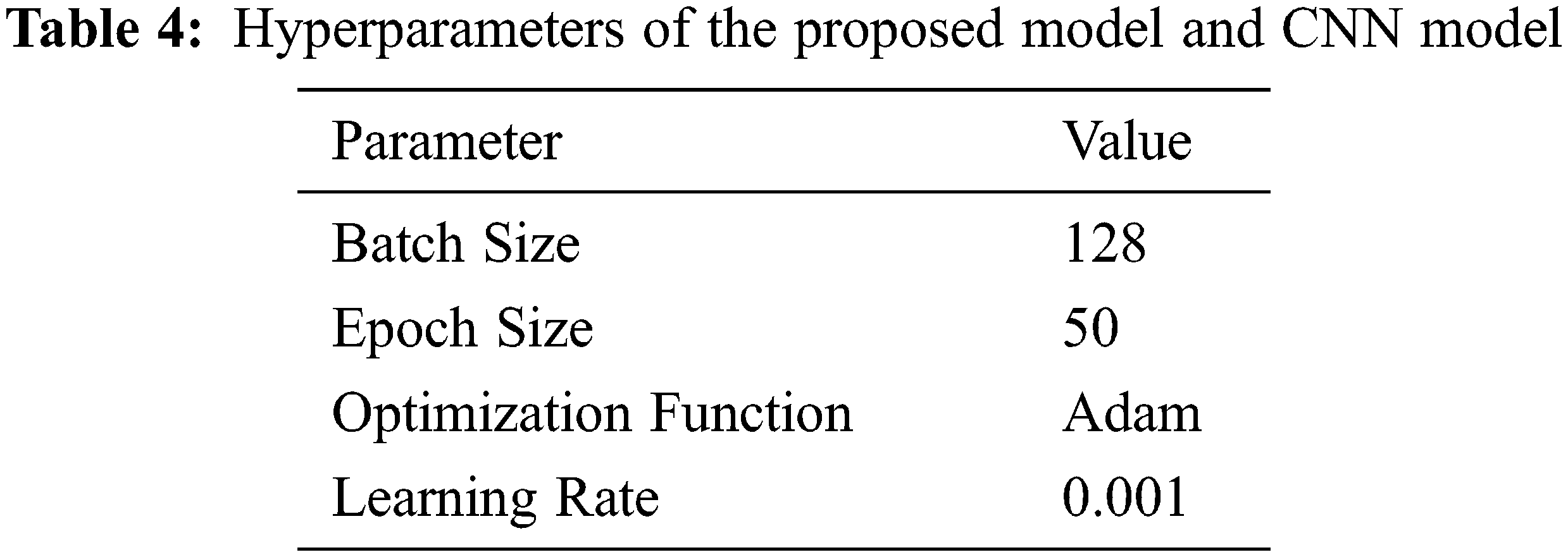
Tab. 4 shows the best values of the hyperparameters used in implementations. The hyperparameters values are chosen after trying different values. The value of the learning rate is usually between 0.0 and 0.1. It affects the model performance significantly, as the small learning rates increase the epochs size because the updates of the weights will be small. On the other hand, high learning rates attract few epochs size due to high speed.
The proposed model was evaluated using six performance metrics: Accuracy, Loss Error, ROC curve, Precision, Recall, and F-measure. These evaluation metrics are defined as follows.
a. Accuracy: the ratio between correctly predicted outcomes and the sum of all predictions. It is calculated as
b. Loss Error: loss error measures the model’s success by predicting the expected outcome. A log loss function is the most popular loss function used for predicted probability
c. ROC Curve: Receiver Operating Characteristic (ROC) curve is a graph to illustrate the model's classification based on TPR or sensitivity and FPR or specificity. Area Under the Curve (AUC) measures the two-dimensional area under the ROC curve. The ROC curve is calculated as
d. Precision: the number of true positives divided by the total number of elements labeled as belonging to the positive class. It is calculated as
e. Recall: Recall or sensitivity is the number of correct results divided by the number of results that should have been returned. It is calculated as
f. F-measure: the Precision and Recall weighted average. It is calculated as
The experimental results depend on four different scenarios. First, a comparative experiment comparing the proposed model with a basic CNN model without solving the imbalanced dataset problem. Second, a comparative experiment comparing the proposed model with a basic CNN model with solving the imbalanced dataset problem. Third, a comparative experiment comparing the proposed model with state-of-the-art machine learning classifiers. Fourth, a comparative experiment comparing the proposed model with the most related works. The results of these experiments are described in the following sections.
4.3.1 Experiment 1: Performance Comparison of the Proposed Model and CNN Model Without Data Balancing
In this experiment, the proposed model is evaluated and compared with the basic CNN model without SMOTE technique. Figs. 6a and 6b show the relationship between the training log loss error and the testing log loss error, and the epochs size. The results show that increasing the epoch size decreases the log loss error. Epoch’s size equal to 50 produce the smallest log loss error, which indicates that the epoch parameter setting of the model structure design is reasonable and can meet the detection requirements. The results also show that the proposed model outperformed the CNN model, which scored 0.14 and 0.16 compared with the CNN model, which scored 0.28 and 0.29 in the model training and model testing. In terms of accuracy, the accuracy increased when the size of epochs increased. The proposed model achieved 91.98% and 91.86% accuracy scores, where the CNN model achieved an accuracy score of 84.95% and 84.79% in the model training and model testing, as shown in Figs. 7a and 7b.
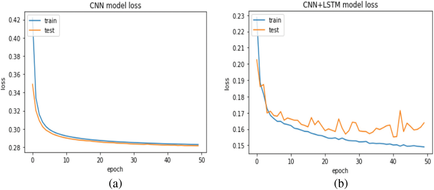
Figure 6: Loss error for (a) CNN model, (b) proposed model without SMOTE
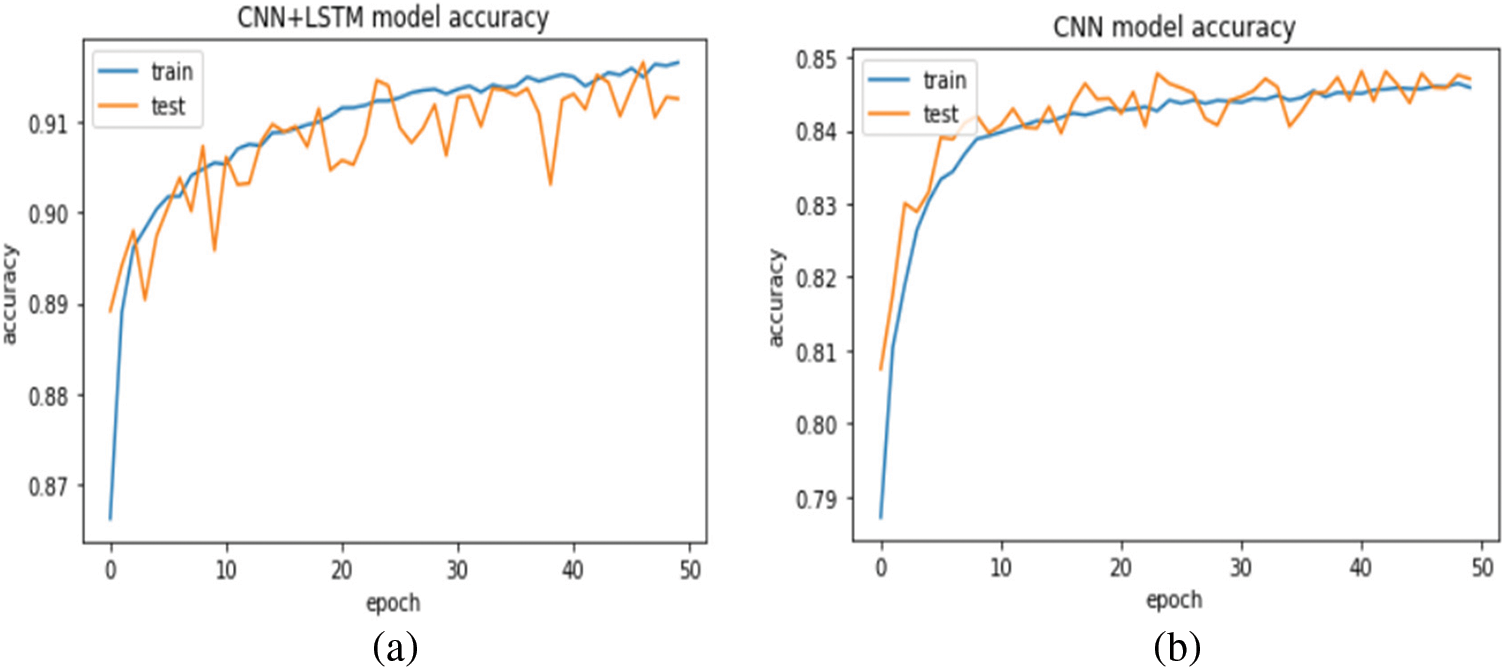
Figure 7: Accuracy for (a) CNN model, (b) proposed model without SMOTE
The confusion matrix is described in Tab. 5, used to evaluate the binary classification on the test set for the imbalanced dataset. For the CNN model, the results show that 4762 attack flows are misclassified among 51244 attack flows which mean that less than 6% of the entire attacks are misclassified. On the other hand, 5900 of 46801 normal flows are misclassified as attacks, indicating less than 8% false alarm rate. For the proposed model, the results show that 3334 attack flows are misclassified among 49500 attack flows which means that less than 4% of the entire attacks are misclassified. On the other hand, 5233 of 40556 normal flows are misclassified as attacks which indicates less than a 5% false alarm rate.
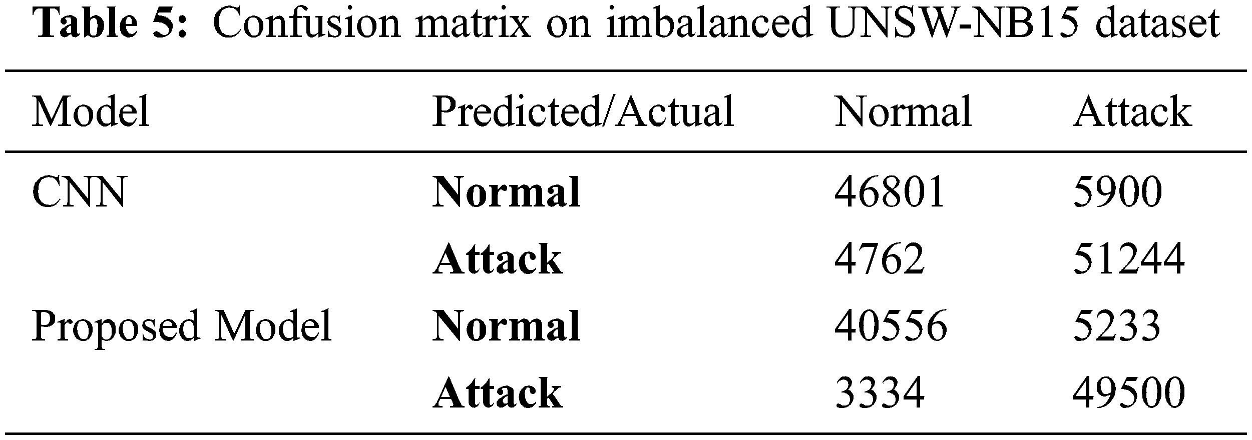
Fig. 8 represents the ROC curve for the results. The ROC curve measures the model validation to detect the attack. The y-axis represents the sensitivity for detecting attacks and normal traffic. The x-axis represents the specificity for detecting attacks only. The confusion matrix and ROC curve proved the effectiveness of the proposed model to detect attacks on the imbalanced dataset. In general, the proposed model outperformed the basic CNN model in the imbalance dataset in the performance metrics.
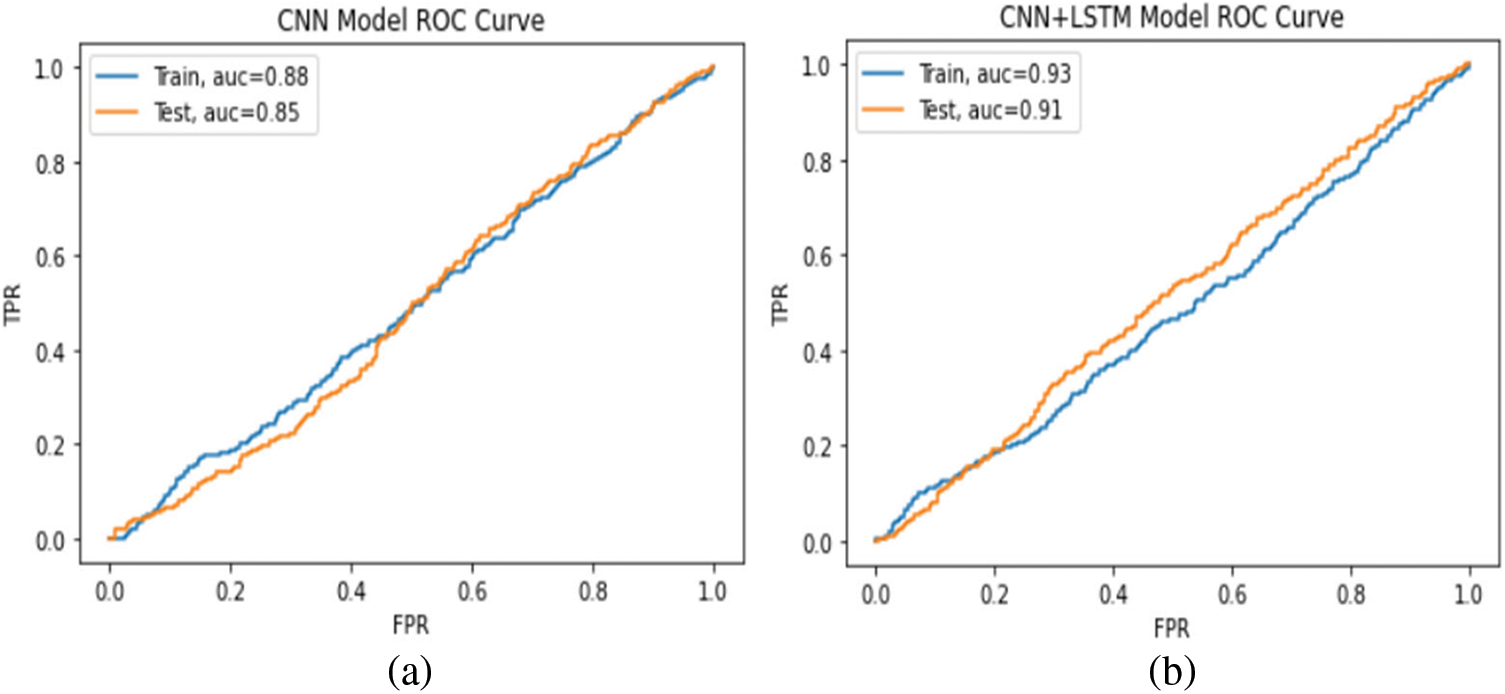
Figure 8: ROC curve for (a) CNN model, (b) proposed model without SMOTE
4.3.2 Experiment 2: Performance Comparison of the Proposed Model and CNN Model with Data Balancing
In this experiment, the proposed model and CNN model are evaluated and compared with the SMOTE technique. Figs. 9 and 10 show the log error loss and accuracy for the balanced dataset. The value of the log error loss for the proposed model is the same with and without data balancing in the model training, but it is decreased in the model testing, which scored 0.15. Also, the proposed model outperformed the CNN model, which scored 0.25 and 0.26 in the model training and model testing, respectively. Although the accuracy is close with SMOTE and without SMOTE in the proposed model, the model without SMOTE does not perform good classification in the test data because of the imbalanced dataset. The proposed model achieved 91.9% and 92.1% accuracy scores, whereas the CNN model achieved 89.8% and 89.9% in model training and testing, respectively.
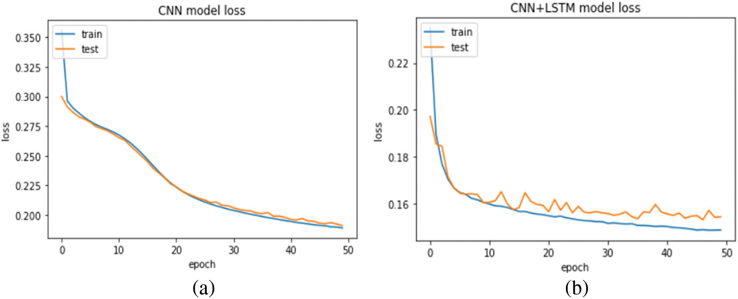
Figure 9: Loss error for (a) CNN model, (b) proposed model with SMOTE
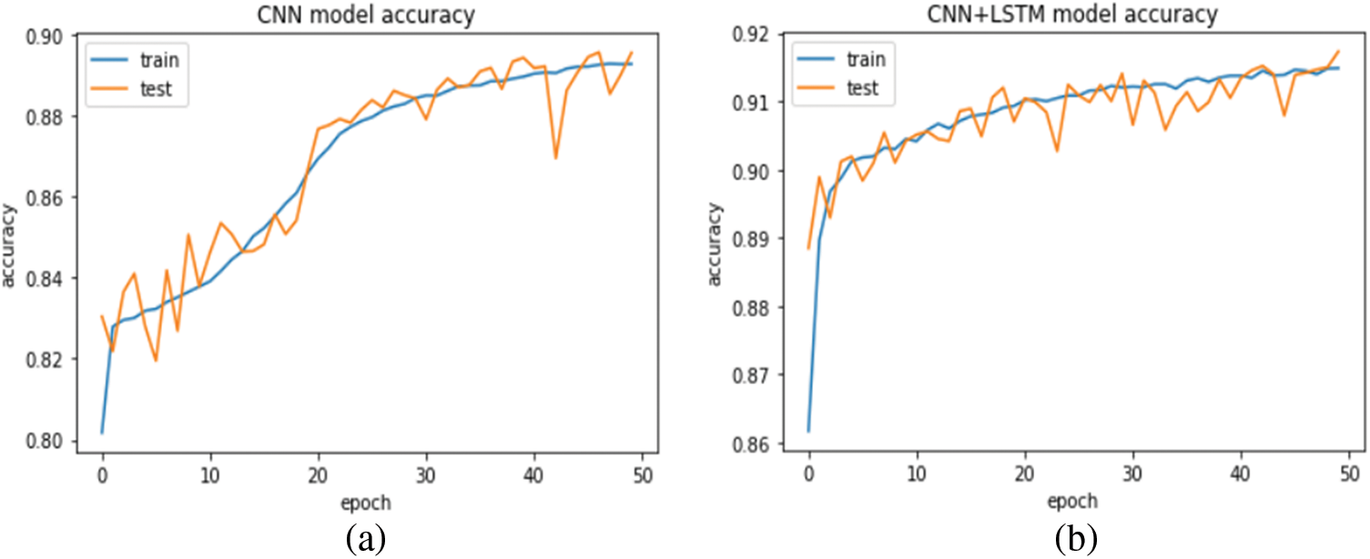
Figure 10: Accuracy for (a) CNN model, (b) proposed model with SMOTE
The confusion matrix is described in Tab. 6, used to evaluate the binary classification on the test set for the balanced dataset. For the CNN model, the results show that 2762 attack flows are misclassified among 52244 attack flows which means that less than 4% of the entire attacks are misclassified. On the other hand, 2103 of 42556 normal flows are misclassified as attacks, indicating a less than 6% false alarm rate. For the proposed model, the results show that 1134 attack flows are misclassified among 52200 attack flows, meaning less than 2% of the entire attacks are misclassified. On the other hand, 3900 of 48301 normal flows are misclassified as attacks, indicating less than a 3% false alarm rate. The applied models were also evaluated using the ROC curve metrics, as shown in Fig. 11. The confusion matrix and ROC curve proved the effectiveness of our model to detect attacks on the balanced dataset.

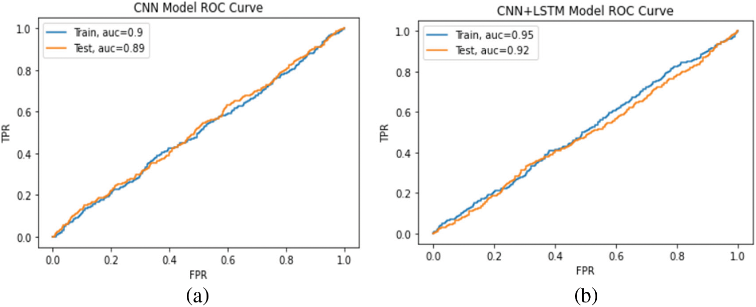
Figure 11: ROC curve for (a) CNN model, (b) proposed model with SMOTE
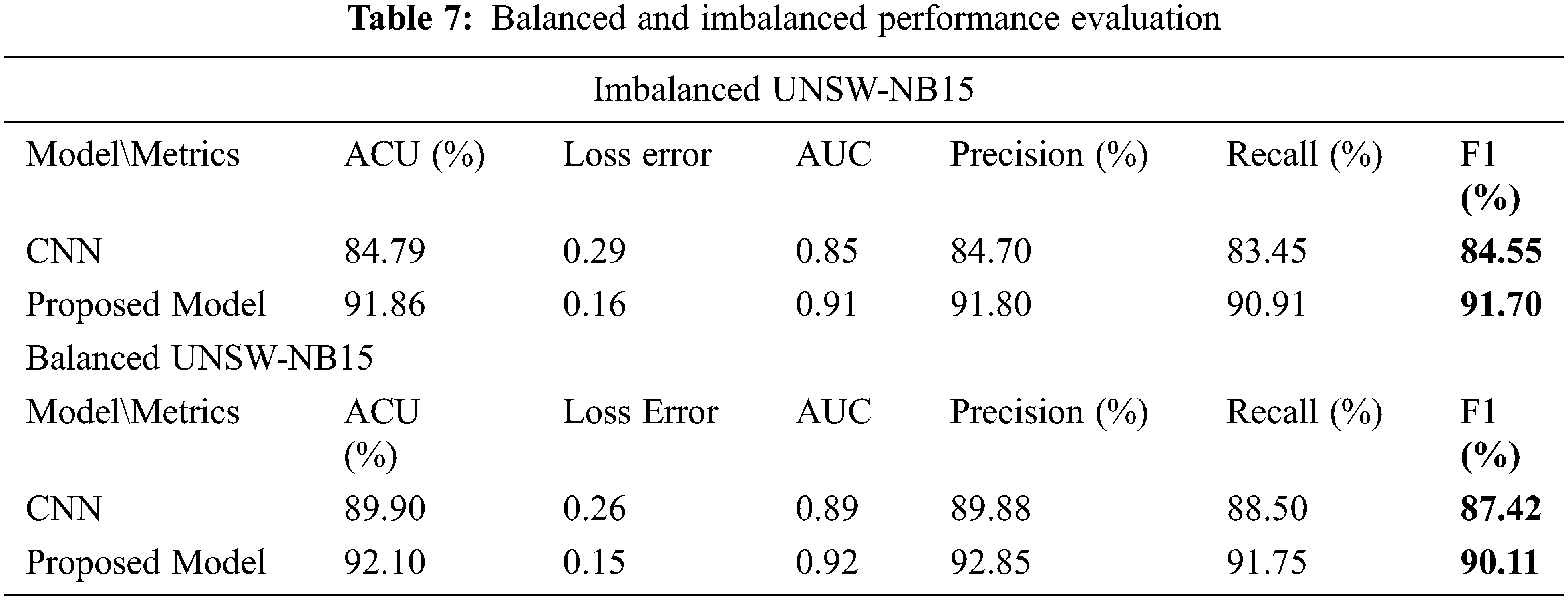
The performance metrics values are shown in Tab. 7 to assess the performance of the models with and without data balancing on the model testing. The results indicate that the proposed model outperformed the CNN model with and without data balancing. Therefore, combining CNN and LSTM improved the classification results. The CNN model is the best for extracting the important features through the condensing of the input data to find the inherent structures and representations in the data. With adding LSTM, the sequence prediction is supported across time, giving us the appropriate classification. Also, the SMOTE technique helps to avoid overfitting problem and enhance the accuracy.
4.3.3 Experiment 3: Performance Comparison of the Proposed Model with the Machine Learning benchmark Classifiers
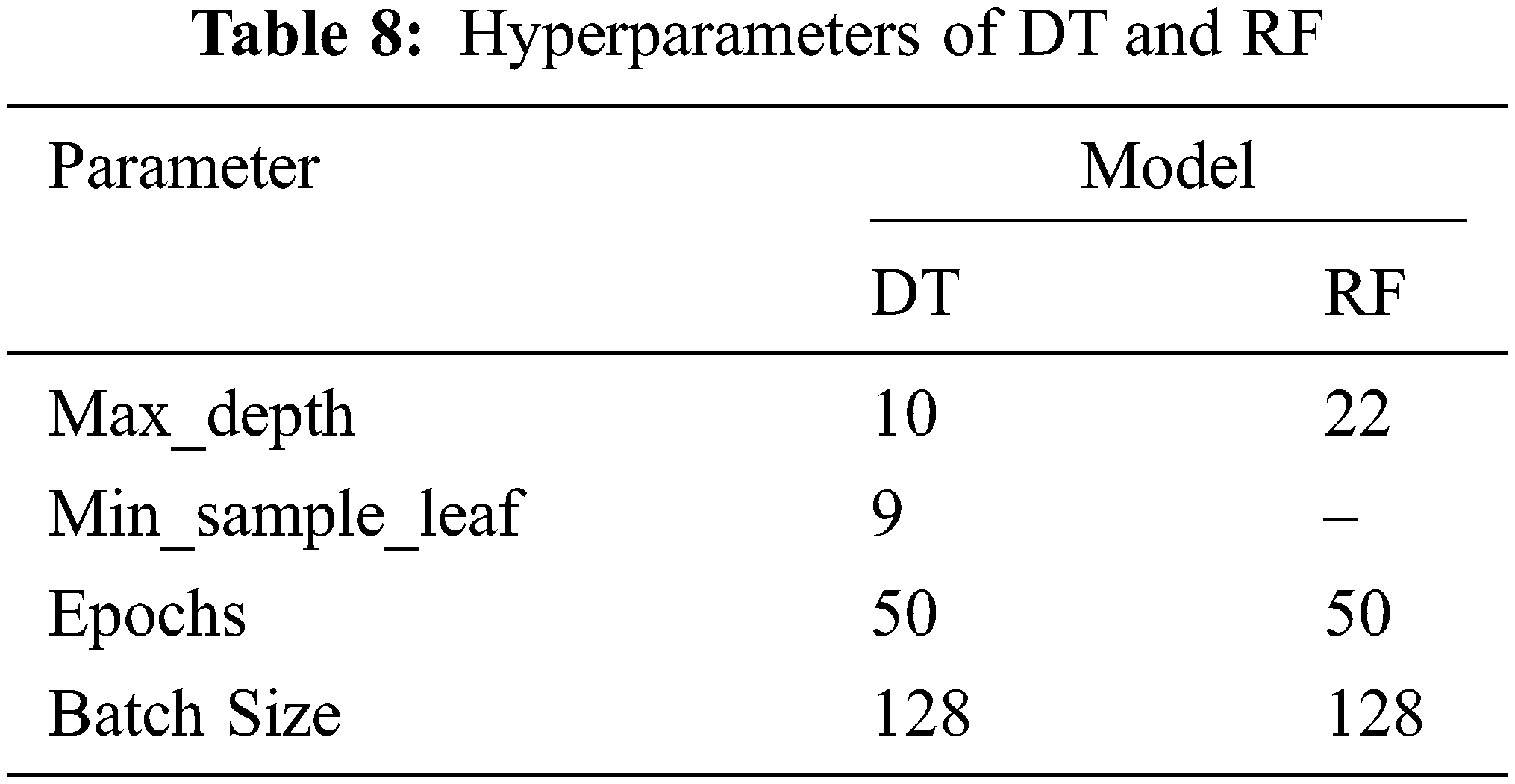
This experiment compares the proposed model with two machine learning classifiers on the balanced dataset. Same data preprocessing, balancing, and performance evaluation of the proposed model are applied to machine learning classifiers. We choose DT and RF classifiers in this experiment, and it is implemented using Scikits Learn (Sklearn) machine learning library. Tab. 8 represents the hyperparameters of the DT and RF classifiers.
A. Decision Tree (DT)
Decision Tree (DT) is a supervised machine learning algorithm. DT is a tree structural model where the features are represented as leaves and branches. Each branch represents the classification outcomes, and each leaf represents the class labels. Root node is the first node in the tree. Tree classification of the input feature is performed by passing it over a tree starting from the root and ending in the leaf. The DT can handle the numerical and categorical data, multioutput problem, and validate a model using statistical tests.
B. Random Forest (RF)
Random Forest (RF) is a supervised machine learning algorithm. RF consists of individual decision trees that work as a group. The RF takes the prediction from each decision tree and takes the best prediction through voting. The RF is well working due to multiple relatively uncorrelated trees operating in a group that will outperform any individual constituent trees. It gives better results because the trees protect each other from their errors. Therefore, the trees that work as a group make the correct decision.
The performance evaluation is performed using the same performance metrics in previous experiments. For DT, we use DecisionTreeClassifier from the Sklearn library. For RF, we use RandomForestClassifier from the Sklearn library. As shown in Fig. 12, the experiment showed that the DT achieved an accuracy of 88.69% and 88.57% in the model training and testing, respectively. In the case of RF, it achieved 90.69% and 90.85% accuracy in the model training and testing, respectively. The applied models were also evaluated using the ROC curve metrics, as shown in Fig. 13.
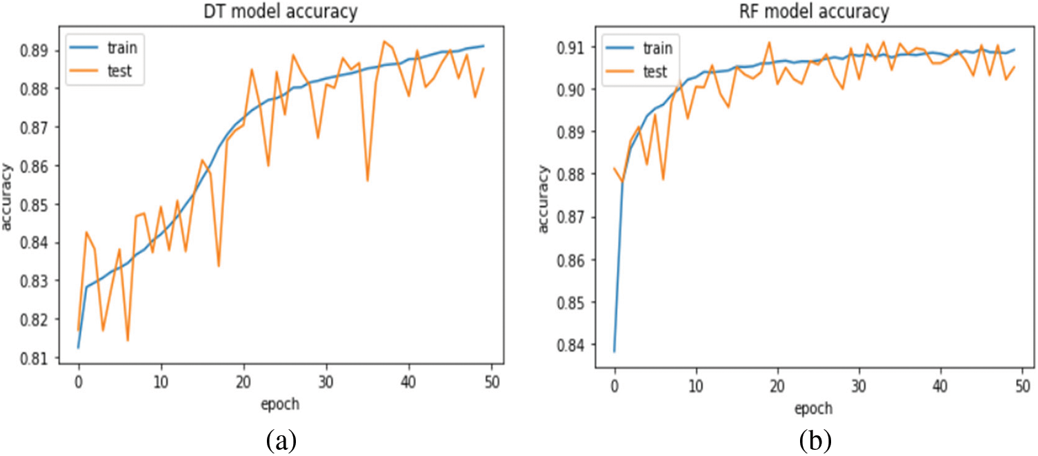
Figure 12: Accuracy for (a) DT model, (b) RF model
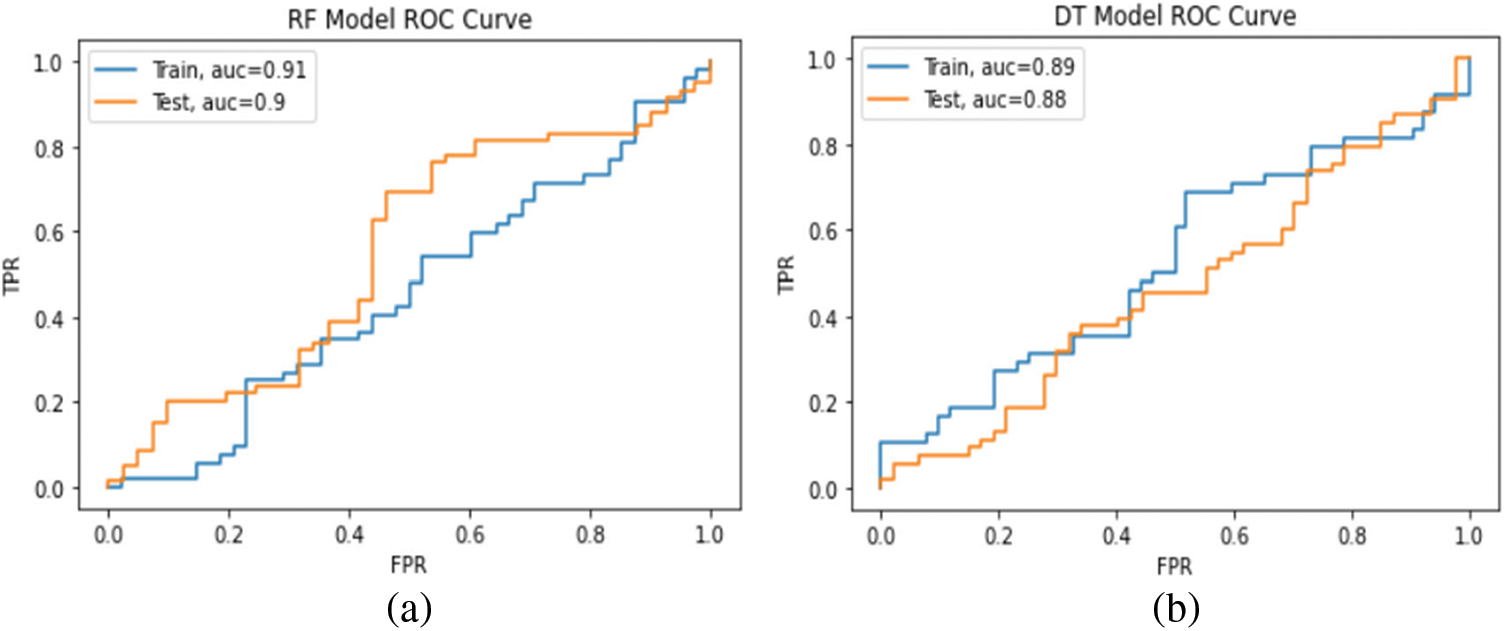
Figure 13: ROC curve for (a) DT model, (b) RF model
In summary, we evaluate the performance of DT, RF, CNN, and the proposed model on a balanced dataset. In the CNN and the proposed model experiment, we trained the models with and without data balancing. The models give us better performance on data balancing, where the proposed model achieved better classification with 92.10% accuracy. In the third experiment, RF achieved better performance than DT with 90.85% accuracy. As shown in Fig. 14, when we compare the proposed model with CNN, DT, RF, it is the best in accuracy, loss error, AUC, precision, recall, and f-measure. Tab. 9 summarizes the proposed model results against the other models on the balanced UNSW-NB15 dataset.
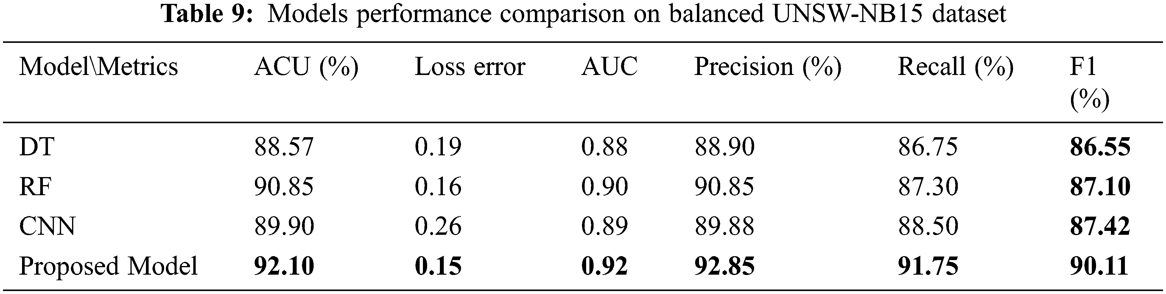
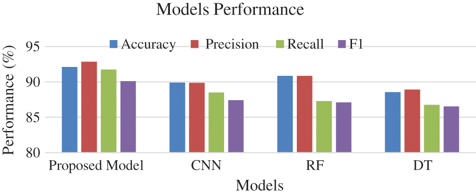
Figure 14: Models performance on balanced data
4.3.4 Experiment 4: Performance Comparison of the Proposed Model with the Most Related Works
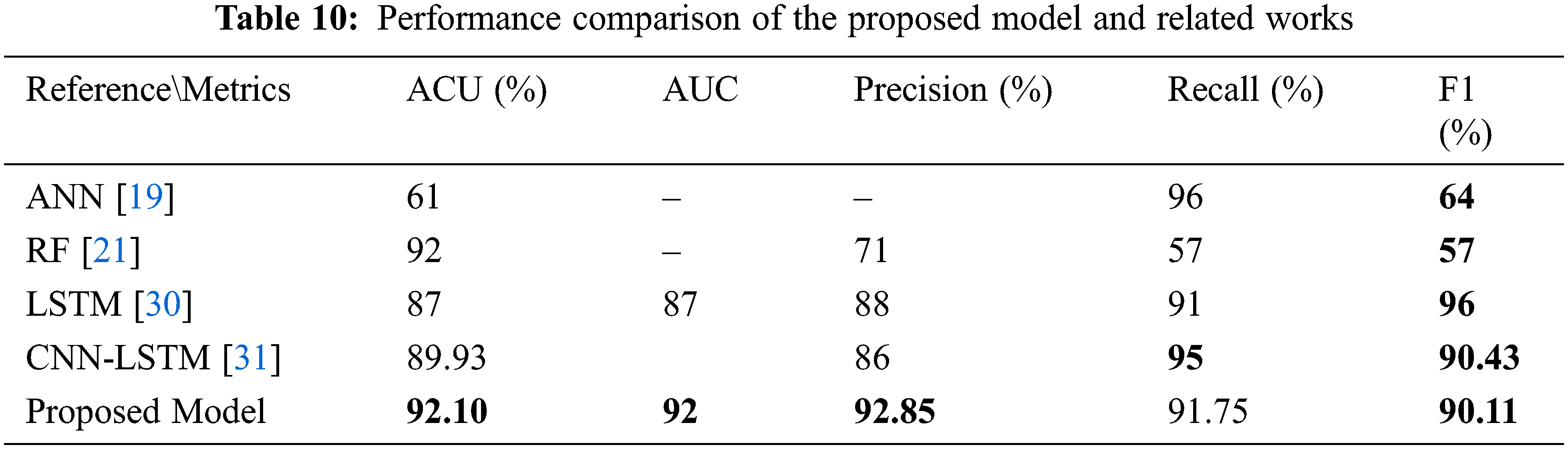
In this experiment, the performance of the proposed model and the related works that solve the imbalanced problem are compared. Different resampling techniques are used on different datasets. When we compare our results with the results that used the UNSW-NB15 dataset, we observe that the proposed model outperformed the model in [31] in terms of accuracy and precision. Also, the proposed model gives reasonable results compared to the rest of the related works. The comparison is presented in Tab. 10.
An Intrusion Detection System (IDS) architecture is developed in this paper based on a combination of a Convolutional Neural Network (CNN) and a Long Short-Term Memory (LSTM) model to detect the security attacks in IoT using the UNSW-NB15 dataset. The missing values in the dataset are removed based on the interpolation method. Additionally, the Synthetic Minority Over-sampling Technique (SMOTE) is implemented to handle the imbalanced dataset to improve the classification. The performance of the proposed model is evaluated based on four experiments: First, we compare the proposed model with the CNN model on an imbalanced dataset. Second, we compare the proposed model with the CNN model on a balanced dataset. Third, we compare the proposed model with DT and RF machine learning classifiers on a balanced dataset. Finally, we compare the proposed model with the most related works. The proposed model achieved 92.10% accuracy, higher than CNN, DT, and RF on the balanced dataset. Moreover, the proposed model gives reasonable results compared to most related works. As future work, we aim to extend the current work to implement deep learning models for multi-class classification on different new network intrusion datasets to validate the proposed model performance.
Acknowledgement: The authors would like to extend their sincere thanks and gratitude to the supervisor for his support and direction of this research.
Funding Statement: The authors received no specific funding for this study.
Conflicts of Interest: The authors declare that they have no conflicts of interest to report regarding the present study.
1. L. M. R. Tarouco, L. M. Bertholdo, L. Z. Granville, L. M. R. Araiza, F. Carbone et al., “Internet of Things in healthcare: Interoperability and security issues,” in 2012 IEEE Int. Conf. on Communications (ICC), Canada, pp. 6121–6125, 2012. [Google Scholar]
2. S. S. Goel, A. Goel, M. Kumar and G. Moltó, “A review of Internet of Things: Qualifying technologies and boundless horizon,” Journal of Reliable Intelligent Environments, vol. 7, no. 1, pp. 23–33, 2021. [Google Scholar]
3. I. Yaqoob, E. Ahmed, I. A. Hashem, A. I. Ahmed, A. Gani et al., “Internet of Things architecture: Recent advances, taxonomy, requirements, and open challenges,” IEEE Wireless Communications, vol. 24, no. 3, pp. 10–16, 2017. [Google Scholar]
4. P. P. Ray, “A survey on Internet of Things architectures,” EAI Endorsed Transactions on Internet of Things, vol. 2, no. 5, pp. 151714, 2016. [Google Scholar]
5. M. Conti, A. Dehghantanha, K. Franke and S. Watson, “Internet of Things security and forensics: Challenges and opportunities,” Future Generation Computer Systems, vol. 78, no. 6, pp. 544–546, 2018. [Google Scholar]
6. M. Kumar, K. Dubey and R. Pandey, “Evolution of emerging computing paradigm cloud to fog: Applications, limitations and research challenges,” in 2021 11th Int. Conf. on Cloud Computing, Data Science & Engineering (Confluence), India, pp. 257–261, 2021. [Google Scholar]
7. A. Karale, “The challenges of IoT addressing security, ethics, privacy, and laws,” Internet of Things, vol. 15, no. 11, pp. 100420, 2021. [Google Scholar]
8. P. E. Elango and S. Subbaiah, “Intrusion detection system performing a distributed novel hybrid intrusion detection framework,” International Journal of Recent Technology and Engineering, vol. 8, no. 211, pp. 454–459, 2019. [Google Scholar]
9. J. Song, H. Takakura, Y. Okabe and K. Nakao, “Toward a more practical unsupervised anomaly detection system,” Information Sciences, vol. 231, no. 4, pp. 4–14, 2013. [Google Scholar]
10. B. Geluvaraj, P. M. Satwik and T. A. Ashok Kumar, “The future of cybersecurity: Major role of artificial intelligence, machine learning, and deep learning in cyberspace,” in Int. Conf. on Computer Networks and Communication Technologies, Garden City University, Bangalore, pp. 739–747, 2019. [Google Scholar]
11. J. Lee, J. Kim, I. Kim and K. Han, “Cyber threat detection based on artificial neural networks using event profiles,” IEEE Access, vol. 7, pp. 165607–165626, 2019. [Google Scholar]
12. X. Wang, Y. Zhao and F. Pourpanah, “Recent advances in deep learning,” International Journal of Machine Learning and Cybernetics, vol. 11, no. 4, pp. 747–750, 2020. [Google Scholar]
13. S. Moyer, “IoT sensors and actuators,” IEEE Internet of Things Magazine, vol. 2, no. 3, pp. 10, 2019. [Google Scholar]
14. H. Khattak, M. Bouhlal, R. Aitabdelouah, S. Elfilali and E. Benlahmar, “Perception layer security in Internet of Things,” Future Generation Computer Systems, vol. 100, no. 7, pp. 144–164, 2019. [Google Scholar]
15. A. Hasan and V. K. Patle, “Security threats in perception and network layer of Internet of Things (IoTA review,” International Journal of Technology, vol. 10, no. 2, pp. 143–152, 2020. [Google Scholar]
16. S. A. Chelloug and M. A. El-Zawawy, “Middleware for Internet of Things: Survey and challenges,” Intelligent Automation and Soft Computing, vol. 24, no. 2, pp. 309–318, 2018. [Google Scholar]
17. H. Akram, D. Konstantas and M. Mahyoub, “A Comprehensive IoT attacks survey based on a building-blocked reference model,” International Journal of Advanced Computer Science and Applications, vol. 9, no. 3, pp. 355–373, 2018. [Google Scholar]
18. M. S. Mahdavinejad, M. Rezvan, M. Barkatain, P. Adibi, P. Barnaghi et al., “Machine learning for Internet of Things data analysis: A survey,” Journal of Digital Communications and Networks, Elsevier, vol. 1, no. 3, pp. 1–56, 2018. [Google Scholar]
19. S. Bagui and K. Li, “Resampling imbalanced data for network intrusion detection datasets,” Journal of Big Data, vol. 8, no. 1, pp. 238, 2021. [Google Scholar]
20. M. Tavallaee, E. Bagheri, W. Lu and A. Ghorbani, “A detailed analysis of the KDD CUP 99 data set,” in 2009 IEEE Symp. on Computational Intelligence for Security and Defense Applications, Canada, pp. 1–6, 2009. [Google Scholar]
21. A. Arif, N. Javaid, A. Aldegheishem and N. Alrajeh, “Big data analytics for identifying electricity theft using machine learning approaches in microgrids for smart communities,” Concurrency and Computation: Practice and Experience, vol. 33, no. 17, pp. 2755, 2021. [Google Scholar]
22. ShieldSquare Captcha, Globaldata.com, 2021. [Online]. Available: https://www.globaldata.com/company-profile/state-grid-corporation-of-china/.[Accessed: 07- Dec- 2021]. [Google Scholar]
23. K. Shankar Komathi Maathavan and S. Venkatraman, “A secure encrypted classified electronic healthcare data for public cloud environment,” Intelligent Automation & Soft Computing, vol. 32, no. 2, pp. 765–779, 2022. [Google Scholar]
24. “KSM Blood Bank,” Accessed on: Jan. 3, 2022. [Online]. Available: https://www.useityellowpages.com/ksm-blood-bank.htm. [Google Scholar]
25. H. Pajouh, R. Javidan, R. Khayami, A. Dehghantanha and K. Choo, “A two-layer dimension reduction and two-tier classification model for anomaly-based intrusion detection in IoT backbone networks,” IEEE Transactions on Emerging Topics in Computing, vol. 7, no. 2, pp. 314–323, 2019. [Google Scholar]
26. L. Dhanabal and S. P. Shantharajah, “A study on NSL-KDD dataset for intrusion detection system based on classification algorithms,” International Journal of Advanced Research in Computer and Communication Engineering, vol. 4, no. 6, pp. 446–452, 2015. [Google Scholar]
27. J. Schmidhuber, “Deep learning in neural networks: An overview,” Neural Networks, vol. 61, pp. 85–117, 2015. [Google Scholar]
28. E. Hodo, X. Bellekens, A. Hamilton and P. Dubouilh, “Threat analysis of IoT networks using artificial neural network intrusion detection system,” in 2016 Int. Symp. on Networks, Computers and Communications (ISNCC), Tunisia, pp. 1–6, 2016. [Google Scholar]
29. G. K. Teyou and J. Ziazet, “Convolutional neural network for intrusion detection system In cyber physical systems,” ArXiv Computer Science, vol. 2, pp. 1905, 2019. [Google Scholar]
30. M. Adil, N. Javaid, U. Qasim, I. Ullah, M. Shafiq et al., “LSTM and Bat-Based RUSBoost approach for electricity theft detection,” Applied Sciences, vol. 10, no. 12, pp. 4378, 2020. [Google Scholar]
31. M. Azizjon, A. Jumabek and W. Kim, “1D CNN based network intrusion detection with normalization on imbalanced data,” in 2020 Int. Conf. on Artificial Intelligence in Information and Communication (ICAIIC), Japan, pp. 218–224, 2020. [Google Scholar]
32. S. Bagui, E. Kalaimannan, S. Bagui, D. Nandi and A. Pinto, “Using machine learning techniques to identify rare cyber-attacks on the UNSW-NB15 dataset,” Security and Privacy, vol. 2, no. 6, pp. 1–13, 2019. [Google Scholar]
33. G. Praveen Ramalingam, R. Arockia Xavier Annie and S. Gopalakrishnan, “Optimized fuzzy enabled semi-supervised intrusion detection system for attack prediction,” Intelligent Automation & Soft Computing, vol. 32, no. 3, pp. 1479–1492, 2022. [Google Scholar]
34. N. Moustafa and J. Slay, “The evaluation of network anomaly detection systems: Statistical analysis of the UNSW-NB15 data set and the comparison with the KDD99 data set,” Information Security Journal: A Global Perspective, vol. 25, no. 1–3, pp. 18–31, 2016. [Google Scholar]
35. A. Fernandez, S. Garcia, F. Herrera and N. Chawla, “SMOTE for learning from imbalanced data: Progress and challenges, marking the 15-year anniversary,” Journal of Artificial Intelligence Research, vol. 61, pp. 863–905, 2018. [Google Scholar]
36. R. Yang, C. Zhang, R. Gao and L. Zhang, “A novel feature extraction method with feature selection to identify golgi-resident protein types from imbalanced data,” International Journal of Molecular Sciences, vol. 17, no. 2, pp. 218, 2016. [Google Scholar]
37. M. Galety, F. Al Mukthar, R. Maaroof and F. Rofoo, “Deep neural network concepts for classification using convolutional neural network: A systematic review and evaluation,” Technium Romanian Journal of Applied Sciences and Technology, vol. 3, no. 8, pp. 58–70, 2021. [Google Scholar]
 | This work is licensed under a Creative Commons Attribution 4.0 International License, which permits unrestricted use, distribution, and reproduction in any medium, provided the original work is properly cited. |