DOI:10.32604/iasc.2023.026564
| Intelligent Automation & Soft Computing DOI:10.32604/iasc.2023.026564 | |
| Article |
Enhanced Disease Identification Model for Tea Plant Using Deep Learning
1Department of Electronics and Communication Engineering, University College of Engineering, Thirukkuvalai, Nagapattinam, Tamilnadu, 610204, India
2Department of Electronics and Communication Engineering, Dr. NGP Institute of Technology, Coimbatore, Tamilnadu, 641048, India
*Corresponding Author: Sivakumar Poruran. Email: sivakumar.poruran@gmail.com
Received: 30 December 2021; Accepted: 27 March 2022
Abstract: Tea plant cultivation plays a significant role in the Indian economy. The Tea board of India supports tea farmers to increase tea production by preventing various diseases in Tea Plant. Various climatic factors and other parameters cause these diseases. In this paper, the image retrieval model is developed to identify whether the given input tea leaf image has a disease or is healthy. Automation in image retrieval is a hot topic in the industry as it doesn’t require any form of metadata related to the images for storing or retrieval. Deep Hashing with Integrated Autoencoders is our proposed method for image retrieval in Tea Leaf images. It is an efficient and flexible way of retrieving Tea Leaf images. It has an integrated autoencoder which makes it better than the state-of-the-art methods giving better results for the MAP (mean average precision) scores, which is used as a parameter to judge the efficiency of the model. The autoencoders used with skip connections increase the weightage of the prominent features present in the previous tensor. This constitutes a hybrid model for hashing and retrieving images from a tea leaf data set. The proposed model will examine the input tea leaf image and identify the type of tea leaf disease. The relevant image will be retrieved based on the resulting type of disease. This model is only trained on scarce data as a real-life scenario, making it practical for many applications.
Keywords: Image retrieval; autoencoders; deep hashing; plant disease; tea leaf; blister blight
Tea is a vital beverage all over the world. India is one of the largest tea-producing countries in the world. Assam and Darjeeling from the east and Ooty and Kerala from the south zone of India cultivate Tea in large quantities. The plant research community focuses on the quality and quantity of tea leaves production. The tea leaf is affected by various diseases, which reduce the production of tea leaves. There are multiple diseases in the tea plant such as Camellia dieback and canker, Camellia flower blight, Root rot, Algal leaf spot, Blister blight, Horsehair blight, Poria root disease (Red root disease), Tea scale Aphids (Tea aphid), Spider mites (Two-spotted spider mite). The research community is identifying tea leaf diseases like blister blight, which causes more loss in tea leaf production. There are many ways for image classification, and one of them is the image retrieval system. The system can rank an image into different categories based on the input image query, and the relevant result image category will be retrieved.
Retrieving information in a short time and with less effort has always been a primary concern for researchers. The gap between tea leaf data and information retrieval is addressed by the proposed model, which is better than the state-of-the-art approaches like Deep Supervised Hashing (DPSH) [1] and Deep hashing Neural Networks (DHNN) [2]. Image Retrieval techniques have been developed over the past few years. In the beginning, images were retrieved based on pixel matching. Then came a revolution when the metadata related to these images was utilized. Now modern-day techniques have even eliminated the use of these metadata. Elimination of metadata led to a reduced effort in manually tagging the pictures for better retrieval. Modern techniques incorporated hashing techniques to obtain a unique signature related to an image. To be more specific about this signature, it is the hamming code of an image compared to other images for proper categorization and retrieval. This hamming code is used as it was used in pairwise similarity. Firstly, the hamming codes are compared, and then the labels are compared, which signifies supervised learning. Based on the matching between labels and the hamming code, the positive and the negative feedback are given for the backpropagation. This method allows us to train the model but not entirely. On the other hand, there are many techniques for hashing. The paper will primarily follow an approach to using autoencoders to learn hash codes. The model is less dependent on transfer learning than state-of-the-art approaches like DPSH and DHNN.
The main objective is to improve the model’s Mean Average Precision Score (MAP) and learn hash codes efficiently. It incorporates the simultaneous learning of the basic structure and autoencoders. This technique outperforms the traditional [3–5] methods as it primarily does not use any handcrafted features. Secondly, the main focus is to learn the hash codes simultaneously with the basic model of the training phase.
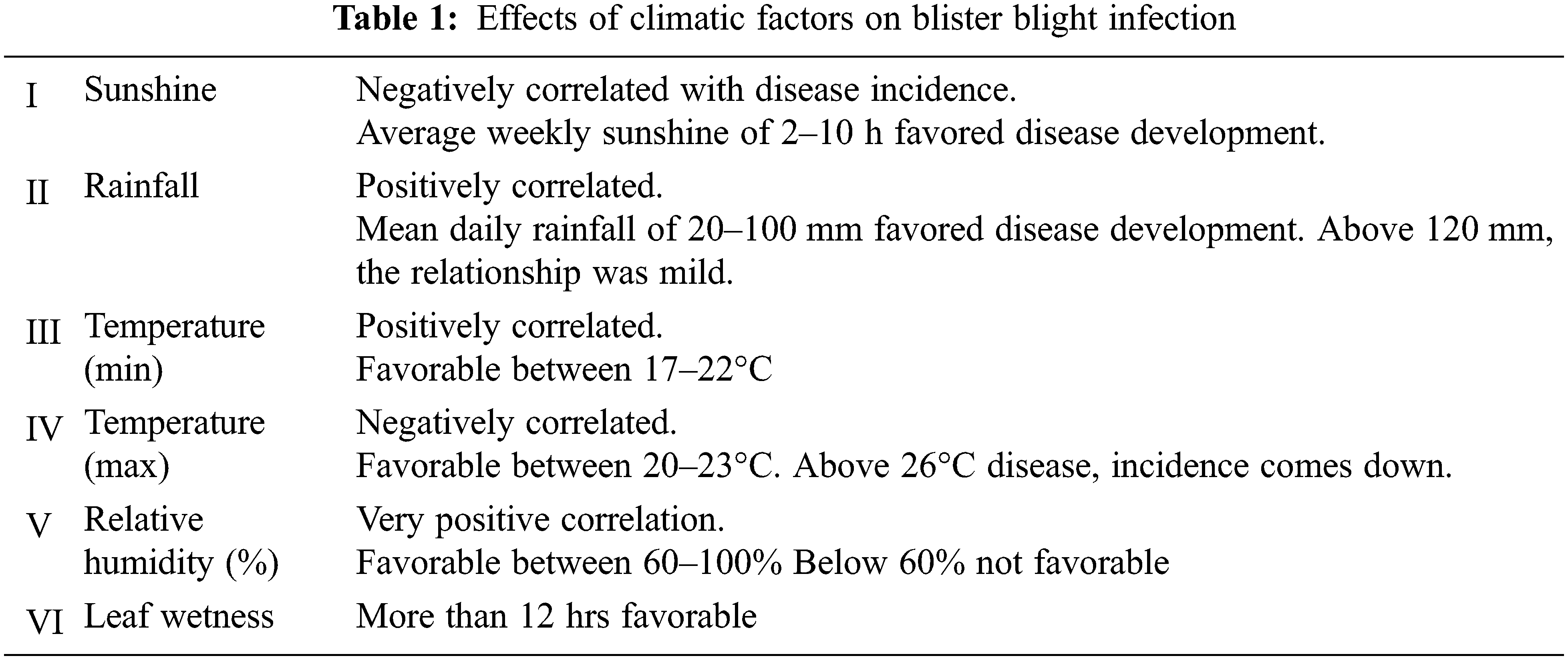
Blister blight is a disease caused by natural climatic conditions. Some of those are mentioned in Tab. 1 (as suggested by the United Planters’ Association of Southern India (UPASI)). All or some of these conditions favor the formation of blister blight. These conditions vary from the usual conditions for the growth of tea leaves.
1.1 The Entry of Pathogen and Symptoms of the Disease
Direct penetration through the upper surface infects only tender leaves and the stem (pluckable shoots). The occurrence of translucent spots, well-developed lesions developed on the upper surface and convex at the lower surface. The upper surface is smooth; the lower surface is first to dull, then becomes grey, and finally pure white. Affected leaves are distorted- irregularly rolled. Stem infections lead to gooseneck shape, die-back, and snapping at the point of infection. This disease can develop in many phases, and there are different methods for controlling these phases. Tab. 2 describes various stages of Blister Blight (as suggested by the United Planters’ Association of Southern India (UPASI)). Blister Blight is the most common disease for tea leaves illustrated in Fig. 1; hence this paper focuses on applying a deep learning model for developing an image retrieval model for the tea leaf disease identification.
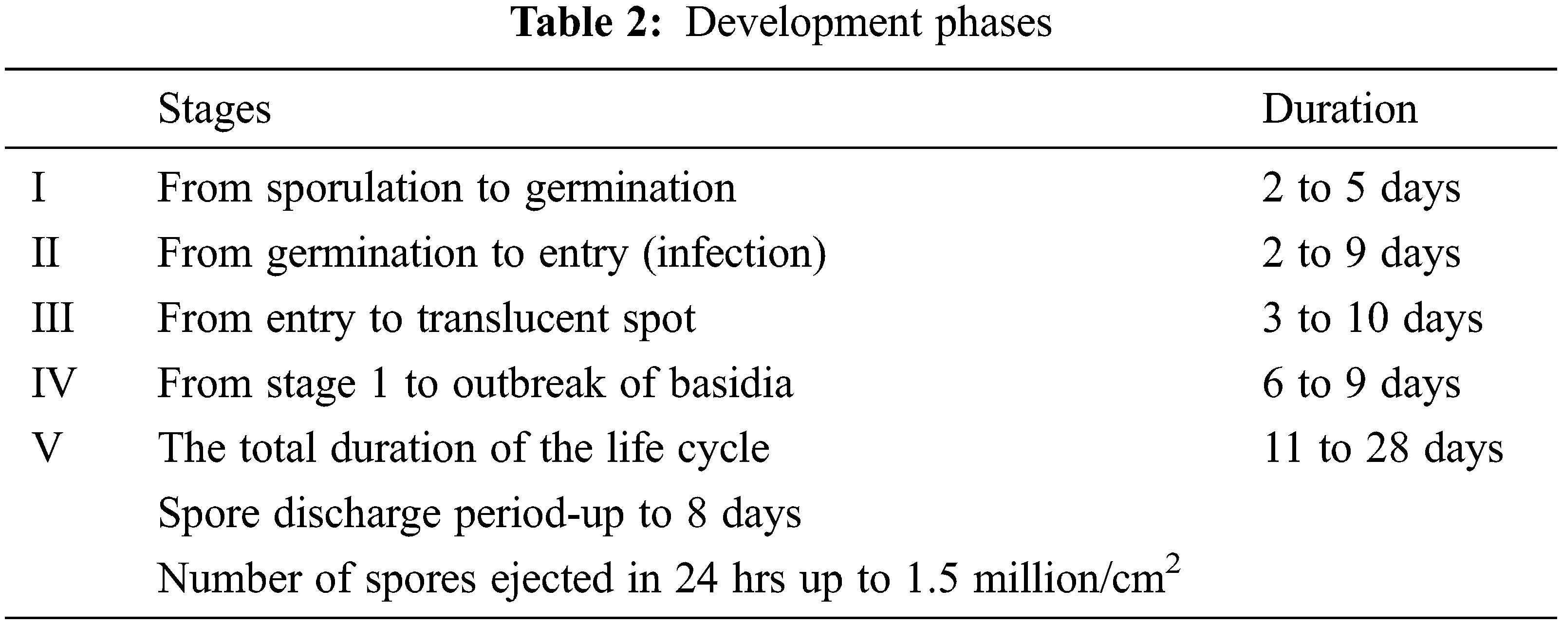
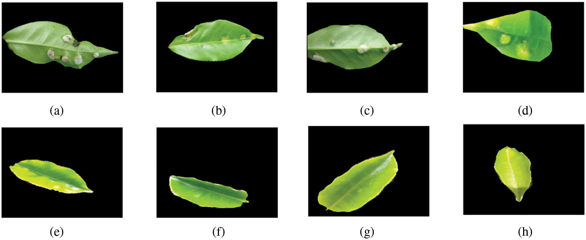
Figure 1: (a) to (d) The front and back faces of a Blister blight Tea Leaf; (e) to (h) The faces of healthy Tea Leaf
Research based on the classification of leaf diseases has been carried out for the past few years, and the fact is that the datasets for such classification are very scarce. This leads to the drawback of underfitting. Many approaches have been developed [6–12]. Most of these approaches relied on manual feature extraction and then applying classification techniques but this also faced curse of dimensionality. As the images were taken from a non-homogenous background, there was a lot of image pre-processing required apart from segmentation. Due to the lack of sample images, these approaches followed data augmentation to train their respective models, leading to overfitting. Some of these approaches [7,10] even require high-quality images for pre-processing and classification, which is not feasible in real-life implementation and practical purposes. DHNN used transfer learning as an effective tool for implementing the hashing for image retrieval. It has two components, i.e., Deep Feature Learning Neural Network (DFLNN) and Hash Learning Neural Network (HLNN) [13]. DFLNN mainly relies on transfer learning from the alexnet or vgg models. It uses five convolution and max-pooling layers whose weights are imported from previously trained models.
These models are trained on a large and sufficient dataset containing 60,000 images. The training is done on 50,000 images, and the testing is done on 10,000 images. HLNN, on the other hand, is a single neuron layer containing 4096 neurons mapped to an output of bits required for hamming distance calculation. The weights of the HLNN are the same as that of the last flattened layer of the previously trained model. This lack of all layers contributes to the scarce reorganization of features for the images. The integrated model is again trained on 6,000 images to get the required hashing. The dependence of this model on transfer learning is very high, and there is no provision to filter out to bare minimum features to identify and categorize images. DPSH is yet another but similar approach to image retrieval. The model is identical to DHNN and hence has the same drawbacks. These models use Lasso Regression and Ridge Regression with dropouts to be checked for overfitting. They also use a weighted sigmoid function to take the feedback from binary vectors, thus creating hamming code. Both the models use a pairwise similarity matrix to get the input for backpropagation.
The overall basic concept on which these models work is that having smaller layers than the original model used in transfer learning creates hashing with layers that only recognize a limited number of valuable features. This implies the model has considered the original weights of these layers with less training on the HLNN portion. These methods are far advanced from the traditional methods [3–5], which used handcrafted features for the supervised learning of hash codes. The previously applied methods incorporated non-simultaneous learning approaches where the features of the image and the hash code were not learned by the model in the same instance, thus complicating the process and making it more time-consuming. The primary focus of these papers was to learn hash codes rather than learning features of the image. The modern methods simultaneously trained the same model for features and hash codes. This is since both the components of feature learning and hash learning were integrated in an end-to-end manner, making them more efficient than the traditional techniques. Another benefit is that these modern methods made the process less complex and less time-consuming. Furthermore, a model is required that is inspired by this current method [14] and is less dependent on transfer learning. This method should not have a rigid structure compared to DHNN. It should be nearly or more efficient than these modern methods. The methods must rely on more training on hash codes rather than transfer learning but should be end-to-end integrated as in the state of the art methods, based on deep neural networks. New techniques have evolved for the classification of the Tea Leaf images.
Autoencoders [15,16] have been employed for the vast datasets. They have shown efficiency in the classification of images. This makes it an essential part of the ongoing research, as once an autoencoder is trained to identify and classify images, it does that efficiently. A wide range of autoencoders [14,15] is employed for this purpose. Another interesting fact is that autoencoders can be used for feature reduction [17]. The autoencoder structure suggests that firstly it converts the data in the form of code with a minimum necessary number of features. Then it decodes to get an output refined form of the data. It is also used for denoising [18,19] and feature selection. Principal Component Analysis (PCA) [19] is restricted to a linear map, while autoencoders can have nonlinear encoders/decoders. Autoencoders are mainly just a simple repurposed feed-forward neural network. In other words, neural networks are large nonlinear functions whose parameters are learned by an optimization method that uses vector calculus. We use PCA [20] while prototyping on considerable datasets to reduce the time taken by computations for small datasets. It can be replaced by a more flexible method such as an autoencoder to improve performance. It has been proved that autoencoders [21] are more flexible than other [22] approaches.
Hashing is another way of using a limited number of features to classify an image. Autoencoders are used for hashing [23], making the model more flexible. Different types of autoencoders can be employed for hashing. Using traditional techniques, hashing using autoencoders also reduces searching for images in a database. This is done by mapping the high dimensional feature vectors to a low dimensional binary feature vector, which speeds up the computation. Integrated hybrid modules [19] are gaining popularity for making models more widespread concerning functionality. The Integrated hybrid module is the usage of one module inside the other. This leads to an increase in the efficiency of these modules combined rather than as individuals. The modules may be integrated into an end-to-end or part of another module. This leads to better feature recognition and efficient training of the models so formed. Any convolutional neural network may learn the features from the image very well but categorizing it as a prominent feature requires a different mechanism like PCA, Linear Discriminant Analysis (LDA), or Autoencoders. Autoencoders for hashing is a new concept as it learns only the prominent features to distinguish images, but the learning should be scarce to create an effect of hashing. To make this hashing effective, usually, the depth of the Autoencoder is not increased too much, and for pointing out scarce features, feedback from the previous layers is needed. The skip connections are introduced to train the autoencoders [24] better. These skip connections give better feedback to the autoencoders for the training. The autoencoders work on the concept of taking input and recreating it in such a manner that the output is similar to the input in the desired aspects. Autoencoder is used as an integrated hybrid module within the convolution neural network. It is used as a convolutional autoencoder and as a linear autoencoder on any one of the fattens layers constituted in the model. Skip connections are used with the Autoencoder to improve its performance in identifying the essential features that distinguish one image from another. The feedback can be given using the pairwise similarity matrix used in DHNN and DPSH.
The basic model requires transfer learning, and the Autoencoder incorporated starts from scratch. The model proposed in this paper requires two types of training: the sufficient dataset and the scarce dataset. The training on good data is done in the model used for transfer learning, and the training on scarce data is done when the described model trains. The seamless integration of the basic model and the Autoencoder end-to-end makes the model more efficient and effective. The entire proposed model will be called deep hashing with integrated autoencoders (DHIA). The components of DHIA are basic model (BM) and autoencoders (AE). This model works efficiently for Tea Leaf image retrieval as the model requires very few images for training. The model is used to classify the image dataset into two categories: blister blight and healthy.
DHIA works in two parts, i.e., training the basic model and training the autoencoders. The model works on training with scarce and sufficient data. The basic model (BM) is trained on sufficient data, and the AE is trained on scarce data. Based on the existing methods, the model uses transfer learning for the basic model and trains only the autoencoders with limited time. BM uses a convolutional neural network to process the images, and the output is fed to the AE where AE recognizes prominent features, and the output of the AE is fed to a mapping function to get the required number of bits; in turn, these bits are used to calculate Hamming distance between the images. The feedback is given to the network using a pairwise similarity matrix. The last layer of autoencoders converts the high dimensional vector obtained using encoding to a binary vector used for mapping. DHIA can be optimized under constraints like binary quantization loss and pairwise similarity.
Considering the image data set as {(Ii, yi) | i = 1, 2, . . . N}, where Ii denotes the image and yi denotes its label, the Similarity matrix θ ∈ R2 × N × N for the given image dataset is specifically defined as
Now taking binary vectors of the image data set, I =
Here Ωi, j =
This helps in distinguishing the images with more precision. The cross-entropy function which is to be minimized is
To identify the relation between the learning of BM and AE learning, the parameter computation of BM and AE are as follows: Let γ denote all parameters of multi-layers of BM, and let {W, v} denote the weights of AE. The given input image Ii, the high-dimensional feature representation of BM can be represented by di = φ (Ii; γ), where di ∈ Rd, and the binary feature as an output of AE can be described as fi = WT di+ v = WT φ (Ii; γ) + v, where fi ∈ Rl, W ∈ Rd×l, and v ∈ Rl. For simultaneously optimizing the BM and AE, the optimization function shown in (2) can be further evaluated into
Here μi,j = fiTfj/P, P is the similarity penalty, and η is the regularization coefficient. Utilizing formula derivation, it is easy to see that P varies with the selection of sigmoid functions. The similarity penalty P is equal to 1 when classic sigmoid is employed, 2 when improved sigmoid is employed, and w = s ⋅ l when a weighted sigmoid function is used (Li et al. 2018), respectively.
The function in (3) takes into consideration the pairwise similarity constraint and the binary quantization loss function. The optimization function used in (3) and (4) is equivalent as they both use the L1 norm to define quantization loss. The DHIA using this norm is referred to as DHIA-L2. In DHIA-L2, the weighted sigmoid function is adopted, and μi,j in (4) is equal to fTifj/w, where w = s ⋅ l is the similarity weight. In contrast, the existing deep hashing method used in [23] employs the classic sigmoid function, which renders μi,j used in (4) equal to fiTfj. The binary quantization loss from the L2 norm is also employed in [23].
For optimizing the functions used in (3) and (4), we use the square of L2 term. This results in (5) which are used in the model.
For an immense amount of training samples, a batch-based learning strategy is widely adopted to optimize DHIA used in (3) and (5). For each iteration, sample a random batch of data until all samples are processed. As B and {γ, W, v} are interdependent in (3) or (5), adopt an alternative way to learn them. Therefore, one parameter is updated while other parameters remain fixed to a particular value. Binary feature vectors B =
Here sign () returns a value as +1 or −1 based on the sign of feature vectors. For backpropagation, we need to calculate the derivatives of the equations so formed. The derivatives for Eq. (5) are computed. For the L2 regularization, the optimization function used in (5) concerning fi is differentiable. The closed-form gradient is given below:
Based on the gradient illustrated in (7), derivatives of the optimization function shown in (5) to {γ, W, v} can be computed from the below derivatives
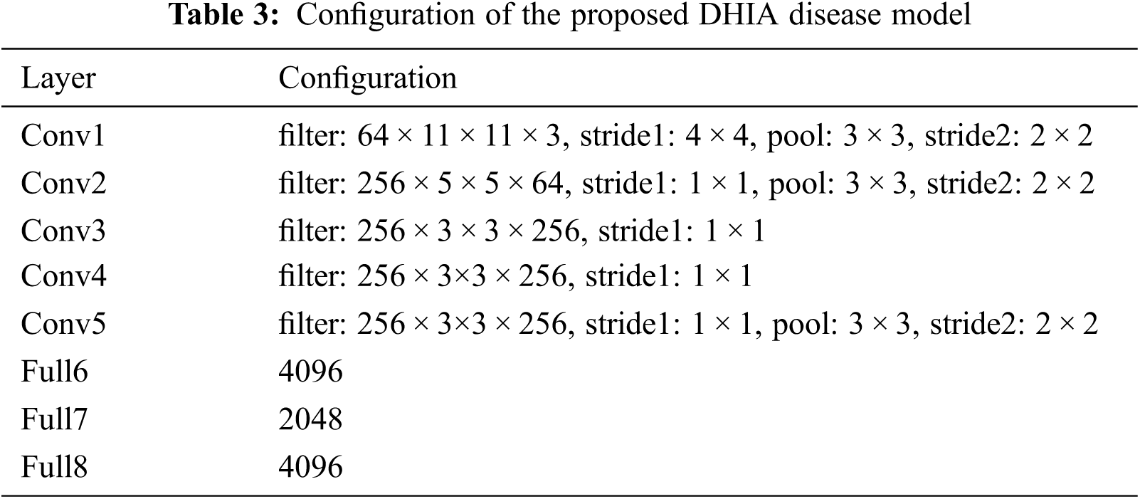
The algorithm and the derivations based on the L2 norms are proposed in DHNNs. The basic model, as in Tab. 3, consists of five convolution layers using max pooling with a filter size of 3 × 3, which takes an input of 256 × 256 images of multiple categories. This portion of the model uses transfer learning to accept the features to form a pre-trained model. Here, alexnet-11 is utilized as our pretrained model. The features and weights in {BM} are obtained using transfer learning from the alexnet model and thus assuring the model is trained on sufficient data. This makes a part of alexnet model efficient as our BM. At the end of the BM we flatten these features to a layer of 4096 neurons.
BM and AE are integrated in an end-to-end manner (shown in Fig. 2), making both the BM and AE to learn simultaneously. Now only scarce data is needed to train our AE portion with the BM model. The advantage of AE is that it only learns the most prominent features rather than all features. As in the structure itself, we are connecting the 4096 neurons obtained from the BM to 2048 neurons resulting in a reduced number of features to create a code. This phase of connecting 4096 neurons to 2048 neurons which results in a reduced number of elements, is known as encoding. The resultant code is then decoded to obtain the hash that will be utilized for getting the hamming distance for the pairwise similarity.
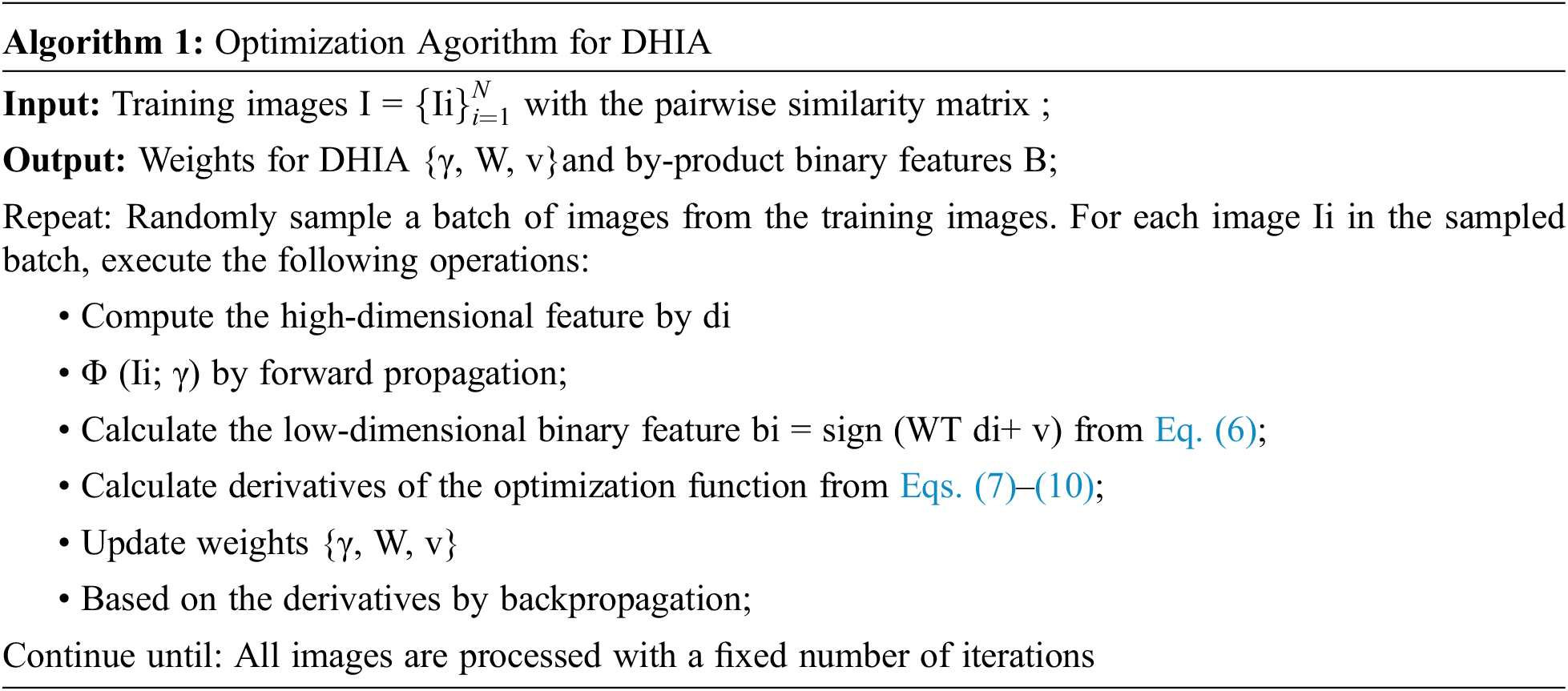
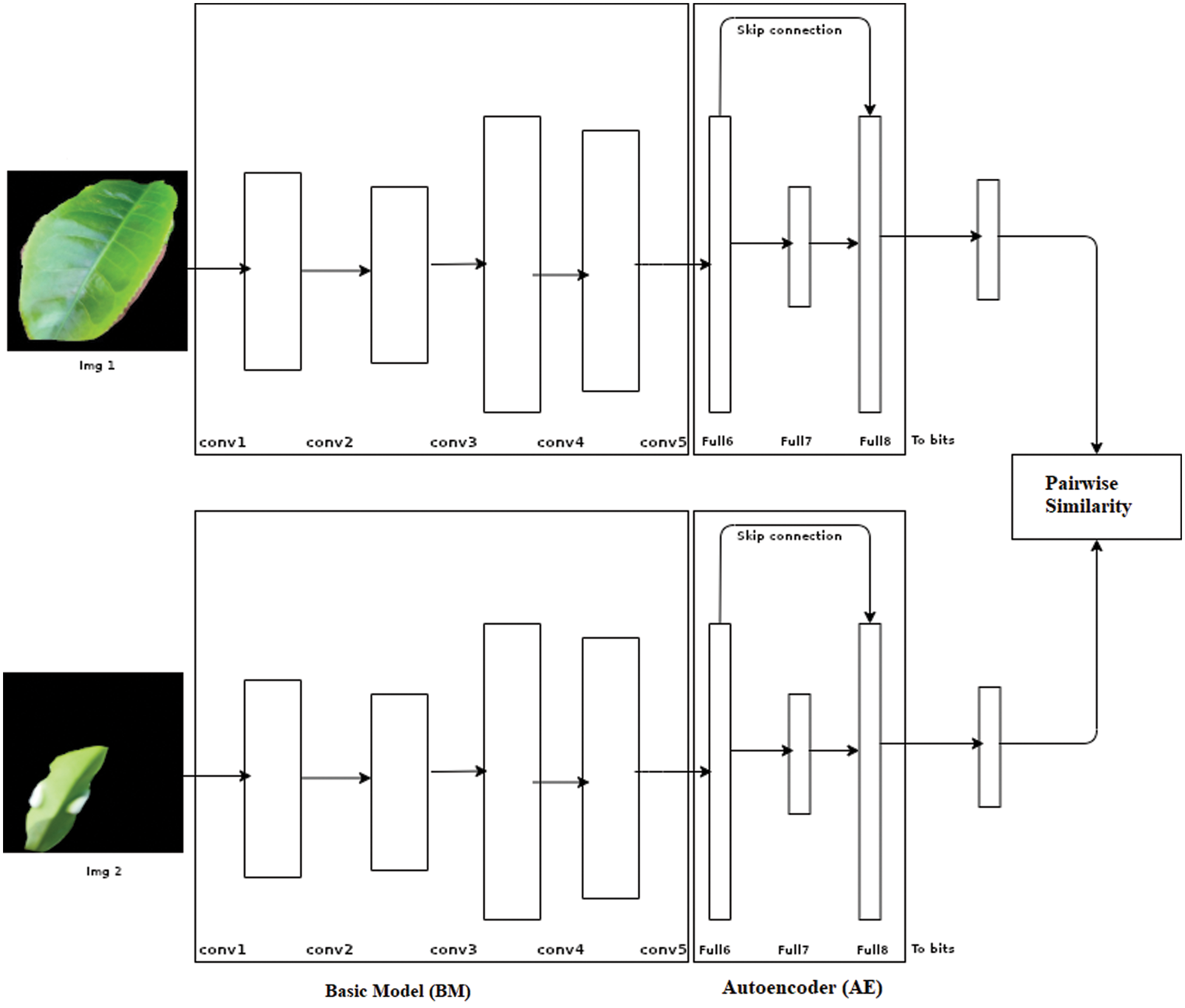
Figure 2: DHIA Architecture
The above-explained structure works well when the dataset contains more distinguishable images in terms of shapes and colours, but if the model includes only small features, then a different approach is to be employed.
The proposed Auto Encoder (AE) learns only small distinguishable features, and these features are enough to separate the images into different categories. As mentioned, these features are very small and may not have a greater weightage in images compared to other features. Thus, the new concept revolves around making these features have more weightage. The solution is straightforward, take a vector containing the normal reward features and add to it the vector containing the small features learned by our AE, which gives increased weight to these small features as if highlighting them. For further simplicity, there is a skip connection from Full6 to Full8. After Full8, the 4096 neurons are mapped to the required number of bits to perform pairwise similarity and check using the hamming distance from these bits. Once the similarity matrix is calculated, the resultant loss is given as feedback to the weight updating of AE as backpropagation. This concept helps in achieving efficient and effective results for the given dataset. Thus, our model uses only important features rather than partial learning that was proposed in previous papers. Partial learning is due to the fact that the last two layers are only trained on a scarce dataset. Learning of only some features leads to hashing that is performed in the AE model. Fig. 2 illustrates the basic architecture used for the model DHIA. The output from autoencoders is converted into the desired number of bits to be further utilized in the pairwise similarity checking.
The Blister Blight disease is season oriented disease that will affect the tea plant in November and December in Tamilnadu, India. The field study is conducted in the Ooty, Tamilnadu. Disease-affected tea leaf images, and healthy images are captured and collected from various tea estates across Ooty with the help of the United Planters’ Association of Southern India (UPSAI). The experiment is conducted on a system with 8 gigabytes of RAM, 512 gigabytes of the solid-state drive as storage, and an i5 8th generation processor. The code is written using PyTorch libraries and python programming language. The IDE used for the execution of the code is spyder. The code is executed for Tea Leaf Dataset for the different number of bits for the pairwise similarity matrix. The similarity factor mentioned in DPSH and DHNN is kept to 0.5.
Tea Leaf dataset is created using the segmentation of images from the captured image using different angles and in different environments. It contains two categories, each containing 76 images. Figs. 3 and 4 illustrate these categories. This dataset is not sufficient even for scarce training; hence the data augmentation procedure is applied as suggested in the previous papers [2]. The images are augmented to a factor of 4 to increase the size of the dataset from 152 images to 608 images. Among these images, 100 images are selected for testing, and the rest 508 images are used for training.
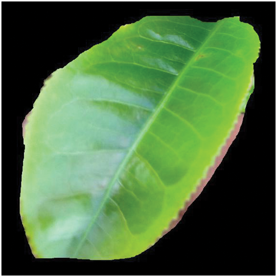
Figure 3: Segmented sample of healthy Tea Leaf
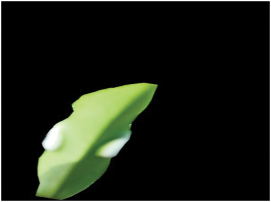
Figure 4: Segmented sample of blight influenced Tea Leaf
3.2 Metric for Performance Evaluation
Precision is the metric that gives an accuracy of the prediction model, and it is defined as the ratio of true positives and the total number of predicted positives. The recall is shown as the ratio of true positives and ground truth positives. Average precision is all about finding the area under the precision-recall curve.
Let n is the number of queries, then the mean of these n queries is referred to as mAP or mean average precision as suggested in the previous papers [25,26]. It is a unique metric used for retrieval systems.
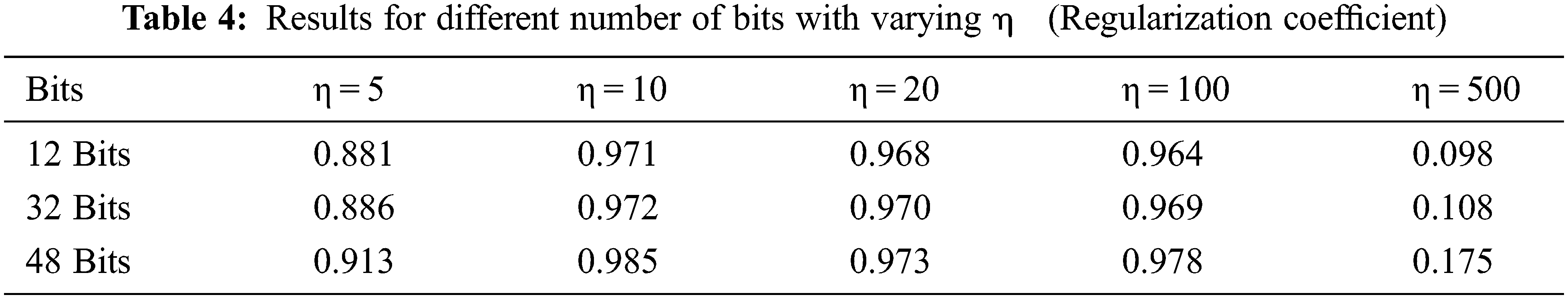
The algorithm used in this model can be fine-tuned with the help of regularization coefficient
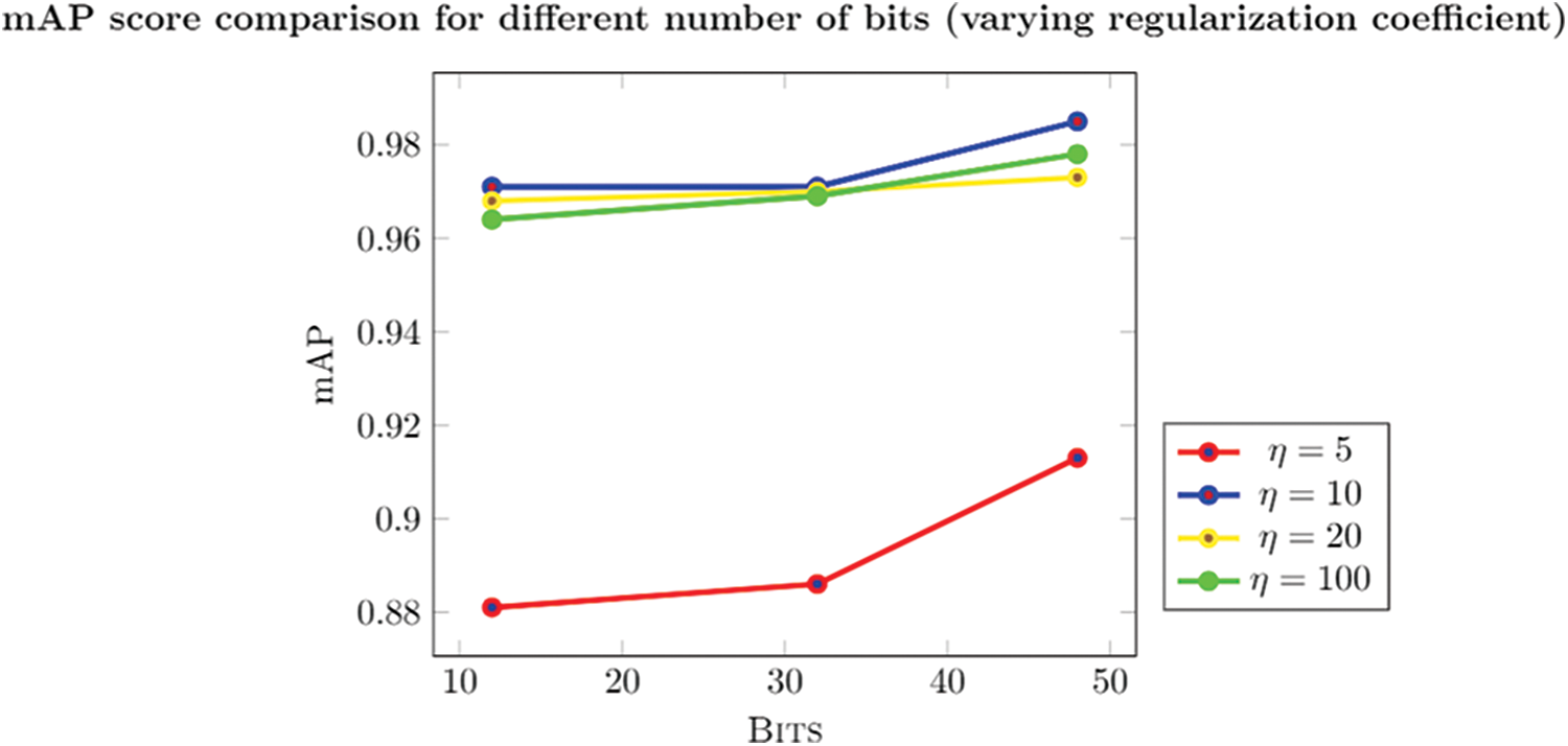
Figure 5: mAPscore with respect to the change in the number of bits with varying regularization coefficient
Apply the proposed model on the different number of bits to check the performance based on the mAP Score.
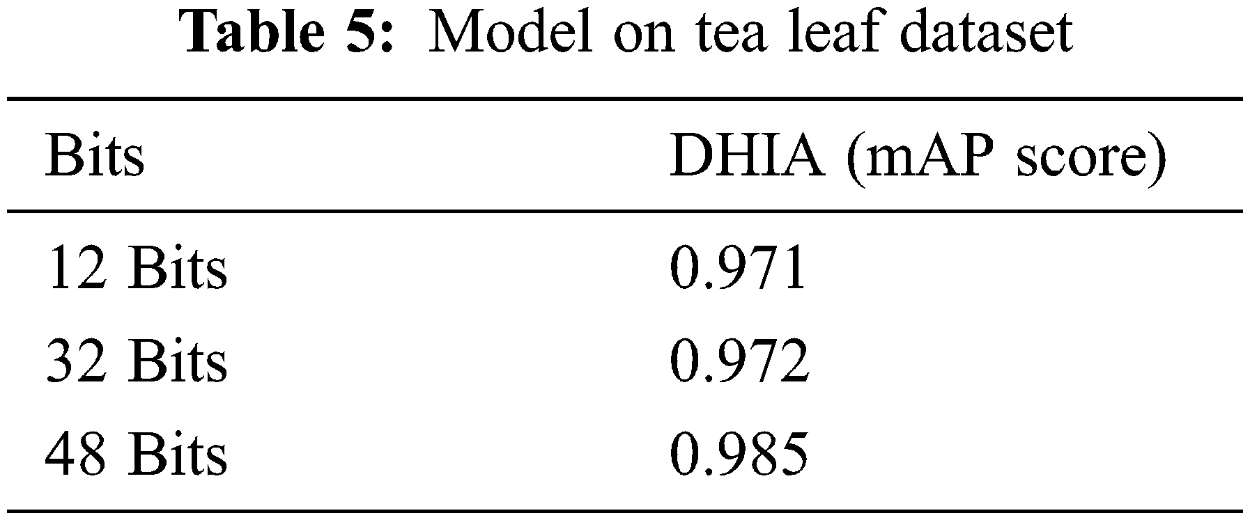
The graph (Fig. 6) for a different number of bits shows how the model is converging to a solution for the different number of bits. It’s easily identifiable that the model usually converges to a solution near to a value that is close to 1; it performs best for 48 bits. The solution usually starts converging at a lower number of epochs (as shown in Fig. 7). The model is trained for 100 epochs to obtain a converge to the solution. Tab. 5 shows that this model performs better when data is augmented as presented by DHNNs. This helps the model to learn these many features in different orientations to make effective predictions.
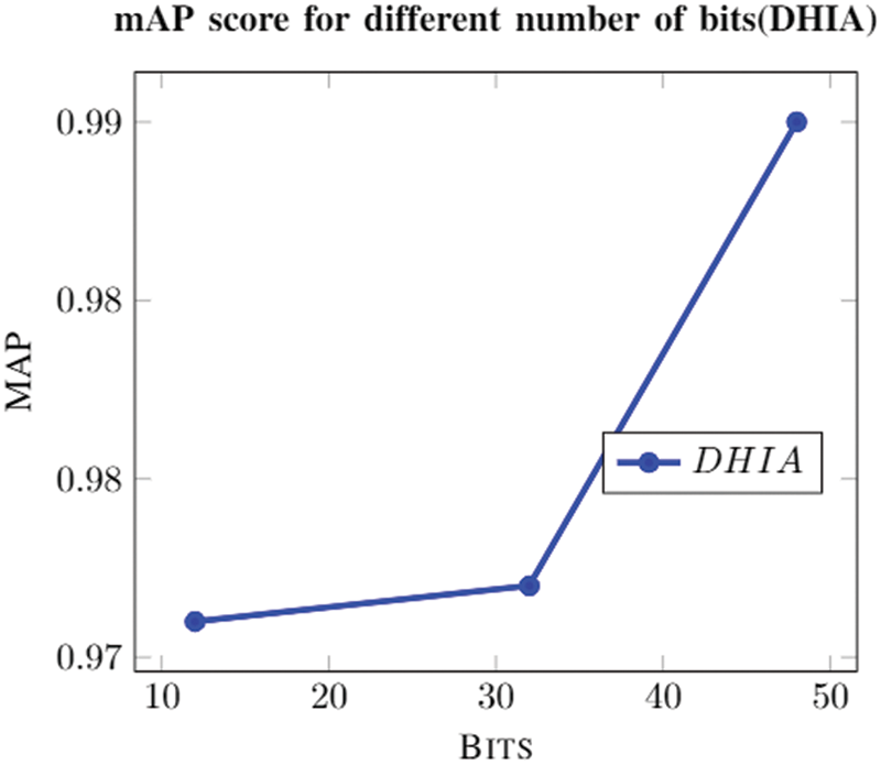
Figure 6: mAP score with the change in the number of bits
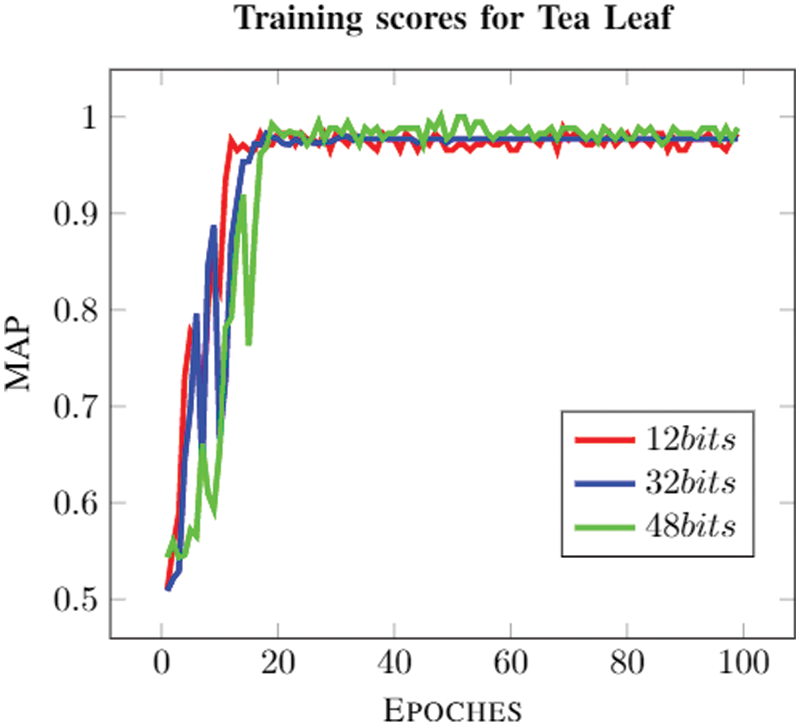
Figure 7: The convergence of the proposed model for Tea Leaf dataset
In the proposed model, autoencoders learn only prominent features required for distinguishing the images between the two respective categories. The dataset that was prepared from random heterogeneous images is only segmented and without any further pre-processing is used in the model for the training. This shows the versatility of the model used for image retrieval. This also suggests that the model is practically useful for real-life applications making it a strong contender for image retrieval and classification. The distinguishing features between both categories are very limited in the case of a bunch of leaves. Training a regular Convolutional Neural Network (CNN) to distinguish these features may produce an underfit model due to the scarce nature of the dataset. Augmentation of the dataset will increase the chance of overfitting and make the model inefficient. On the other hand, the use of an Artificial Neural Network (ANN) requires the selection of features manually, which always leads to the curse of dimensionality. The proposed model is neither under fitted nor overfitting, which is evident from the results that the training mAP scores are near to one, which eliminated the possibility of underfitting nor for overfitting, the training and testing mAP scores are merely at a difference of five units. This makes the model used in the paper more efficient than any of these discussed primitive methods.
The model used is a hybrid between transfer learning, encoding-decoding, and CNNs. It is well illustrated from Fig. 6 that there is a steep increase in mAP score as an increase in the number of bits. This is due to the fact that more bits can be used to fine-tune the model. The model is learning features properly and is well evident from Fig. 7; it shows that there is less noise. The gradient used for training is Stochastic Gradient Descent (SGD) which explains the noise encountered during training. Higher mAP scores in the model show us that it can very well fetch the desired image from the database with minimal false positives and true negatives; it shows that a model is optimal for image classification based on the image reorganization of the model. Furthermore, it shows that the proposed DHIA model is a better choice for classification rather than the usual CNN. The proposed model outperforms than ANNs and CNNs with good retrieval results with less fraction of time using hamming codes.
The model is also trained for various values of the regularization coefficient, keeping the similarity factor at a constant value of 0.5; this value of similarity factor is proven to be efficient in previous models (Y. Li 2018). The regularization coefficient may vary in the range of 10 to 100, as discussed in the results. Thus giving a value of η as 10 for the experiment is evident from Fig. 5.
Designing and developing a disease identification model using the computational approach is key research in the plant research domain. This paper addressed and proposed a novel disease identification image retrieval model for Tea leaf using deep hashing with Integrated Autoencoders. The tea plant is affected by various diseases, but blister blight disease causes major damage to the tea leaf, and it affects tea production. The proposed model identifies and classifies the given tea leaf image as healthy or blister blight. The main contribution of this paper is introducing the Autoencoder in the image retrieval systems for disease identification. Experiments on the above-mentioned datasets show that DHIA outperforms other modern methods to achieve a better performance in image retrieval applications. The mean average precision score is used as a metric to evaluate the performance of the model. The model performance is evaluated based on the number of bits and the regularization coefficient. For future work, the proposed model will experiment with the bare minimum number of layers required for transfer learning and lowering the dependence on transfer learning to train the Autoencoders to get more precise results by only isolating important features that distinguish these images into different categories. The proposed model will be tested for other types of tea leaf disease in the future.
Acknowledgement: The authors would like to thank United Planters’ Association of Southern India (UPASI) for providing us with the necessary help in obtaining the images for the dataset from the Tea Estate.
Funding Statement: The authors received no specific funding for this study.
Conflicts of Interest: The authors declare that they have no conflicts of interest to report regarding the present study.
1. W. J. Li, S. Wang and W. C. Kang, “Feature learning based deep supervised hashing with pairwise labels,” in Proc. of Int. Conf. on Artificial Intelligence (IJCAI’16), New York, pp. 1711–1717, 2016. [Google Scholar]
2. Y. Li, Y. Zhang, X. Huang, H. Zhu and J. Ma, “Large-scale remote sensing image retrieval by deep hashing neural networks,” IEEE Transactions on Geoscience and Remote Sensing, vol. 56, no. 2, pp. 950–965, 2018. [Google Scholar]
3. W. Zhou, Z. Shao, C. Diao and Q. Cheng, “High resolution remote-sensing imagery retrieval using sparse features by auto-encoder,” Remote Sensing Letters, vol. 6, no. 10, pp. 775–783, 2015. [Google Scholar]
4. Z. Du, X. Li and X. Lu, “Local structure learning in high resolution remote sensing image retrieval,” Neurocomputing, vol. 207, pp. 813–822, 2016. [Google Scholar]
5. W. Zhou, S. Newsam, C. Li and Z. Shao, “Learning low dimensional convolutional neural networks for high resolution remote sensing image retrieval,” Remote Sensing, vol. 9, no. 489, pp. 489–509, 2017. [Google Scholar]
6. B. C. Karmokar, M. S. Ullah, M. K. Siddiquee, and K. M. R. Alam, “Tea leaf diseases recognition using neural network ensemble,” International Journal of Computer Applications, vol. 114, pp. 975–8887, 2015. [Google Scholar]
7. S. Hossain, R. M. Mou, M. M. Hasan, S. Chakraborty and M. A. Razzak, “Recognition and detection of tea leaf’s diseases using support vector machine,” in Proc. of Int. Conf. on Signal Processing & Its Applications (CSPA), Batu Feringghi, pp. 150–154, 2018. [Google Scholar]
8. Y. Sun, J. Li, W. Wang, A. Plaza and Z. Chen, “Active learning based autoencoder for hyperspectral imagery classification,” in Proc. of Int. Conf. on Geoscience and Remote Sensing Symp. (IGARSS), Beijing, pp. 469–472, 2016. [Google Scholar]
9. R. Meena, G. P. Saraswathy, G. Ramalakshmi, K. H. Mangaleswari and T. Kaviya, “Detection of leaf diseases and classification using digital image processing,” in Proc. of Int. Conf. on Innovations in Information, Embedded and Communication Systems (ICIIECS), Coimbatore, India, pp. 1–4, 2017. [Google Scholar]
10. C. G. Dhaware and K. H. Wanjale, “A modern approach for plant leaf disease classification which depends on leaf image processing,” in Int. Conf. on Computer Communication and Informatics (ICCCI), Coimbatore, India, pp. 1–4. IEEE, 2017. [Google Scholar]
11. S. D. Khirade and A. B. Patil, “Plant disease detection using image processing,” in Proc. of Int. Conf. on Computing Communication Control and Automation, Pune, pp. 768–771, 2015. [Google Scholar]
12. X. Sun, S. Mu, Y. Xu, Z. Cao and T. Su, “Image recognition of Tea leaf diseases based on convolutional neural network,” in Proc. of Int. Conf. on Security, Pattern Analysis, and Cybernetics (SPAC), Jinan, China, pp. 304–309, 2018. [Google Scholar]
13. Y. Li, L. Xu and T. Liu, “Unsupervised change detection for remote sensing images based on object-based mrf and stacked autoencoders, in Proc. of Int. Conf. on Orange Technologies (ICOT), Melbourne, Australia, pp. 64–67, 2016. [Google Scholar]
14. A. Ding and X. Zhou, “Land-use classification with remote sensing image based on stacked autoencoder,” in Proc. of Int. Conf. on Industrial Informatics-Computing Technology, Intelligent Technology, Industrial Information Integration (ICIICII), Wuhan, China, pp. 145–149, 2016. [Google Scholar]
15. V. Stojnic and V. Risojevi¢, “Analysis of color space quantization in split-brain autoencoder for remote sensing image classification,” in Proc. of Symp. on Neural Networks and Applications (NEUREL), Belgrade, pp. 1–4, 2018. [Google Scholar]
16. W. Wang, Y. Huang, Y. Wang and L. Wang, “Generalized autoencoder: A neural network framework for dimensionality reduction,” in Proc. of Int. Conf. on Computer Vision and Pattern Recognition Workshops, Columbus, OH, pp. 496–503, 2014. [Google Scholar]
17. J. Liu and Y. H. Yang, “Denoising auto-encoder with recurrent skip connections and residual regression for music source separation,” in Proc. of Int. Conf. on Machine Learning and Applications (ICMLA), California, USA, pp. 773–778, 2016. [Google Scholar]
18. B. Zhu, W. Yang, H. Wang and Y. Yuan, “A hybrid deep learning model for consumer credit scoring,” in Proc. of Int. Conf. on Artificial Intelligence and Big Data (ICAIBD), Chengdu, pp. 205–208, 2018. [Google Scholar]
19. S. N. Borade and R. P. Adgaonkar, “Comparative analysis of PCA and LDA,” in Int. Conf. on Business, Engineering and Industrial Applications, Kuala lampur, Malaysia, pp. 203–206, 2011. [Google Scholar]
20. H. Lee, Z. H. Wu and Z. Zhang, “Dimension reduction on open data using variational autoencoder,” in Proc. of Int. Conf. on Data Mining Workshops (ICDMW), Singapore, pp. 1080–1085, 2018. [Google Scholar]
21. Q. Fournier and D. Aloise, “Empirical comparison between autoencoders and traditional dimensionality reduction methods,” in Proc. of Second Int. Conf. on Artificial Intelligence and Knowledge Engineering (AIKE), Sardinia, Italy, pp. 211–214, 2019. [Google Scholar]
22. M. A. Carreira-Perpinán and R. Raziperchikolaei, “Hashing with binary autoencoders,” in Proc. of Conf. on Computer Vision and Pattern Recognition, Bostan, MA, USA, pp. 557–566, 2015. [Google Scholar]
23. H. Zhu, M. Long, J. Wang and Y. Cao, “Deep hashing network for efficient similarity retrieval,” in Proc. of AAAI Conf. on Artificial Intelligence, North America, 2016. [Google Scholar]
24. G. Zhao, J. Liu, J. Jiang, H. Guan and J. R. Wen, “Skip-connected deep convolutional autoencoder for restoration of document images,” in Proc. of Int. Conf. on Pattern Recognition (ICPR), Beijing, pp. 2935–2940, 2018. [Google Scholar]
25. H. Liu, R. Wang, S. Shan and X. Chen, “Deep supervised hashing for fast image retrieval,” International Journal Computer Vision, vol. 127, pp. 1217–1234, 2019. [Google Scholar]
26. F. Shen, C. Shen, W. Liu and H. Tao Shen, “Supervised discrete hashing,” in Proc. of Int. Conf. on Computer Vision and Pattern Recognition (CVPR), Boston, MA, pp. 37–45, 2015. [Google Scholar]
 | This work is licensed under a Creative Commons Attribution 4.0 International License, which permits unrestricted use, distribution, and reproduction in any medium, provided the original work is properly cited. |