Intelligent Automation & Soft Computing DOI:10.32604/iasc.2023.026393
Article

No-Reference Blur Assessment Based on Re-Blurring Using Markov Basis

Gurwinder Kaur* and Ashwani Kumar

Yadavindra Department of Engineering, Punjabi University Guru Kashi Campus, Talwandi Sabo, 151 302, Punjab, India
*Corresponding Author: Gurwinder Kaur. Email: gurwinder_ycoe@pbi.ac.in
Received: 24 December 2021; Accepted: 16 February 2022

Abstract: Blur is produced in a digital image due to low pass filtering, moving objects or defocus of the camera lens during capture. Image viewers are annoyed by blur artefact and the image's perceived quality suffers as a result. The high-quality input is relevant to communication service providers and imaging product makers because it may help them improve their processes. Human-based blur assessment is time-consuming, expensive and must adhere to subjective evaluation standards. This paper presents a revolutionary no-reference blur assessment algorithm based on re-blurring blurred images using a special mask developed with a Markov basis and Laplace filter. The final blur score of blurred images has been calculated from the local variation in horizontal and vertical pixel intensity of blurred and re-blurred images. The objective scores are generated by applying proposed algorithm on the two image databases i.e., Laboratory for image and video engineering (LIVE) database and Tampere image database (TID 2013). Finally, on the basis of objective and subjective scores performance analysis is done in terms of Pearson linear correlation coefficient (PLCC), Spearman rank-order correlation coefficient (SROCC), Mean absolute error (MAE), Root mean square error (RMSE) and Outliers ratio (OR). The existing no-reference blur assessment algorithms have been used various methods for the evaluation of blur from no-reference image such as Just noticeable blur (JNB), Cumulative Probability Distribution of Blur Detection (CPBD) and Edge Model based Blur Metric (EMBM). The results illustrate that the proposed method was successful in predicting high blur scores with high accuracy as compared to existing no-reference blur assessment algorithms such as JNB, CPBD and EMBM algorithms.

Keywords: Blur score; blur variance; objective scores; re-blurred image; subjective scores

1  Introduction

The computational models accept the challenging task of image quality assessment. For digital image processing systems, it is also a necessary task to measure the blur, noise and other degradations in an image and assess its quality [1,2]. For quality assessment of images, an image quality assessment approach is used. In this approach, two types of assessment methods are used: subjective and objective evaluation methods. The subjective image quality assessment approach necessitates the use of human observers to judge the quality of image. For real world applications, this method is very slow, expensive and also dependent on the viewing conditions. The perceptual image quality can be automatically predicted by computational models in objective image quality evaluation methods. This procedure is quicker than subjective evaluation and requires fewer human observers [3]. Objective image quality assessment methods can evaluate the appropriate parameters from the digital image. Full-reference image quality assessment (FR-IQA), Reduced-reference image quality assessment (RR-IQA) and No-reference image quality assessment (NR-IQA) are the three types of objective image quality assessment methodologies that are classified depending on the availability of reference images. In order to calculate the quality scores, FR-IQA needs the reference/original. RR-IQA uses a set of extracted features from a reference image as partial information to evaluate the quality of an image. In the case of NR-IQA, just distorted images are required for image quality evaluation and the reference image is not required. As a result, NR-IQA is extremely beneficial in practical applications when reference images are unavailable.

The metrics based on the edge analysis, which firstly examine the total number of blurred edges in an image and then gradient threshold was applied to remove the faint edges. Sobel edge detector was used for the edge detection [4–7] and local blur values were averaged to find the global blur [4]. Following this method of edge detection, no-reference blur detection was implemented by using Point spread function (PSF) [8], standard deviation-based metric [9] and statistical analysis [10]. The sharpness of the no-reference image was also measured using a quick method based on the highest local variance with respect to its eight neighbors [11]. The gradient magnitude statics followed by the Extreme learning machine (ELM) was also modelled to find no-reference blur score [12]. The Gradient profile sharpness histogram (GRAPH) [13], probability summation model [5] and CPBD [6] method were among the metrics that used the unique notion of JNB based on contrast threshold values for edge detection. Various edge detection methods like global edge detection method [14], wavelet transform method [15], psychometric function was followed by JNB concept to construct the edge map and then Discrete cosine transform (DCT) histogram of blurred image was used to find the final blur metric [16]. The drawbacks of JNB and CPBD methods were overcome by EMBM method based on parametric edge model [17].

The wavelet transform was also used to obtain the detail of horizontal/vertical directions of the image and then the Average cone ratio (ACR) method was used for the calculation of blurriness metric [18]. The Fourier transform is followed by Support vector machine (SVM) model [19] and Wavelet transform followed by magnitude/gradient methods [20] to calculate the blur score. The novel statistical feature extraction on the basis of Zero crossing rate (ZCR) followed by Non-linear regression tool (NLREG) model [21]. For spatially varying blur, the Contrast based blur invariant features (CBIF) based method, multi-resolution concept [22] and Double-density dual tree two-dimensional Wavelet transformations (D3TDWT) based on the wavelet transform also implemented for edge analysis [15]. There are some metrics which were also used block-based blur detection instead of the edge detection [23]. The sharpness metrics are calculated based on Local phase coherence (LPC) [24] and separable discrete wavelet transform and log energies [25]. Various other models based on the image decomposition based on the singular value decomposition [26], Haar wavelet transform based Multi-resolution value (MSV) decomposition [27] and contourlet transformation/image gradients followed by Laplacian pyramid [28] was also designed to calculate the no-reference blur metric. Some metrics are based on the re-blurring concept using strong low pass filter [29], radial analysis in frequency domain method [30] and training free metric [31] followed by shape difference of histogram bins [32] were implemented to calculate no-reference metrics. To find the local motion blur in the selected area, a block based discrete cosine transform method also known as local DCT method followed by the deblurring process was implemented [33]. For naturally and artificially blurred images, the power spectrum of Fourier transform was used to detect the partial blur from histograms and then quality of the image was assessed. To distinguish between noisy and blurred images, Fourier spectrum based Cumulative distribution function (CDF) was used [34].

The Screen image quality evaluator (SIQE) approach was used to estimate the visual quality of screen content images using a training-based Support vector regression (SVR) model [35]. To quantify the blur scores, the training-based SVR model was employed with the Local gradient patterns (LGP) technique, Entropy-based no-reference image quality assessment (ENIQA) method and multi-scale local features approach [36–38]. A neural network-based SVR was also utilized to predict image quality through a separate no-reference image quality evaluation approaches [39,40]. Because Deep convolutional neural networks (DCNN) are trained on a huge number of data sets, they are unable to forecast the quality of pictures with various forms of distortions. A deep meta-learning-based no-reference IQA measure was developed to solve this challenge [41].

We proposed an improved no-reference blur detection algorithm for distorted images, based on the re-blurring concept. According to the first step of the proposed method, a special mask is developed by using the concept of Markov Basis and the Laplace filter. In the second step, the distorted image is re-blurred by using the special mask. For each test and re-blurred image, the local variation in horizontal and vertical pixel intensity is computed. The difference between test and re-blurred images in terms of vertical and horizontal variance is assessed. The maximum value from the horizontal and vertical blur score has been considered as the final blur score.

The rest of the paper is split into four sections. The second section provides an overview of existing approaches. The third section elaborates the Markov basis and proposed no-reference blur assessment method. Fourth section discusses the performance parameters and how they are being used to evaluate the proposed algorithm. The whole work is concluded in fifth section.

2  Introduction to Markov Basis and Proposed Algorithm

A review on the concepts of Markov Basis, basic moves and contingency tables is presented in this section, which will use in the development of proposed algorithm.

2.1 Markov Basis

Consider, a finite set I and it consists of n number of elements that is n = |I|. Each element that belongs to a finite set I is termed as a cell and same abbreviated as i ∈ I. The cell i is ofttimes multi-index that is i = i1, i2, i3………im. The frequency of the cell xi is always denoted by the non-negative integer xi ∈ N where N = {1, 2, 3, 4……..}. A contingency table is the set of all cell frequencies x = {xi}i∈I. A contingency table x = {xi}i∈I ∈ Nn and it is formed by non-negative integers of n-dimensional column vector. The sample size is denoted as |x|=∑i∈Ixi and it is defined by L1-norm of x ∈ Nn. If Z is a set of integer numbers, then ap becomes a fixed column vector consisting of integer numbers that is ap ∈ Zn where p = 1, 2, 3…..m. A m-dimensional column vector t = (t1, t2….., tm) ′ ∈ Zm as tp=ap′x,p=1,2,……,m . Where ′ indicates the transpose of the matrix and vector. The matrix A defined by m × n matrix dimensions, with its p-row being ap′ given by A=[a1′⋮am′] and if t = Ax is a column vector of m-dimensions. The set T is expressed as T = {t:t = Ax, x ∈ Nn} = ANn ⊂ Zm [42].

For the self-supporting model of two-way contingency tables, similar tests are performed by the set of x′ s for specified t, A−1[t] = {x ∈ Nn:Ax = t}(t-fibers), where t is the row and column sums of x. The set of x′ s is represented by A−1[t], which has the same number of row and column sums to t. The decomposition Nn is given by the set of t-fibers. The set of t-fibers are Kernel dependent and Kernel is denoted as Ker(A). The set of t-fibers are same, if different A′s having the same Ker(A).The equivalence relation is defined by x1 ∼ x2 ⇔ x1 − x2 ∈ Ker(A). The Nn is subdivided into disconnected equivalence classes. The set of these equivalence classes produces the set of t-fibers [42].

A move is defined by n-dimensional column vector of integers m = {mi}i∈I ∈ Zn, if column vector is in Ker(A). There are two parts of a move m, one is the positive part m+={mi+}i∈I and the second is the negative part m−={mi−}i∈I . Both parts are interpreted by mi+=max(mi,0) and mi−=max(−mi,0) respectively. The move m is the difference between its positive and negative part i.e., m = m+ − m−, also m, m+ and m− ∈ Nn. Furthermore, m+ and m− are in same t-fiber, m+, m− ∈ A−1[t] for t = Am+ = Am−. The sample size of m+ or m− defines the degree of m as deg⁡(m)=|m+|=|m−| . For the given A, the set of moves denoted by M=MA=Zn∩Ker(A) [43].

For all t, A−1(t) composes one B equivalence class, a set of finite moves B is named as Markov Basis. Moreover x1, x2 ∈ A−1[t], B ⊂ MA and x2 is accessible from the x1 by B if the sequence of moves m1, m2……, ms ∈ B. If ɛs ∈ [ − 1, 1], s = 1, 2, ….., S, such that x2=x1+∑s=1Sϵsms , here x1+∑s=1Sϵsms∈A−1[t] for 1 ≤ s ≤ S. The Markov basis to generate n×n3 -contingency tables by using its elements have been found in For n ≥ 6(n be the multiple of 3), let xj ∈ A−1[t] where j = 1, 2, 3, …….k are the representative elements for n×n3 -contingency tables [43]. B becomes a set of moves that is {m1, m2, m3…….mk} and zp is a matrix of dimension n×n3 , where p = 1, 2, 3, ….., k. The zp has three rows and n3 columns that is this matrix either has two columns (1,−1,0)′,(−1,1,0)′,((1,0,−1)′,(−1,0,1)′or (0,1,−1)′,(0,−1,1)′) and + zp represents the remaining zero columns. The two columns also be ( − 1, 0, 1) ′, (1, 0, − 1)′, ((− 1, 0, 1)′, (1, 0, − 1)′ or (0, 1, − 1)′, (0, 1, − 1)′) and − zp represents the remaining zero columns. In matrix form, the + zp or − zp can be represented as given below:

[1−10−110000],[−1100001−10],[0001−10−110],[−1101−10000],[−1100001−10]and[000−1101−10]

A one-dimensional column vector represents all the elements of B, where B is known as Markov basis and its elements are known as moves. Each element of one-dimensional column vector can be written as follows:

zp = (z1, z2, ….., zn) ′, m = 1, 2, 3, ….., k and zs = 1 or − 1 or 0 such that if s=1,2,3,…….n3

zs={ 1ifzs+n3+zs+2n3=−1and∑i=1i≠sn3zi=−1−1ifzs+n3+zs+2n3=1and∑i=1i≠sn3zi=10ifzs+n3+zs+2n3=0and∑i=1i≠sn3zi=0} (1)

if s=n3+1,n3+2,n3+3,…….2n3

zs={ 1ifzs−n3+zs+2n3=−1and∑i=n3+1i≠sn3zi=−1−1ifzs−n3+zs+2n3=1and∑i=n3+1i≠sn3zi=10ifzs−n3+zs+2n3=0and∑i=n3+1i≠sn3zi=0} (2)

if s=2n3+1,2n3+2,2n3+3,…….n3

zs={ 1ifzs−2n3+zs−n3=−1and∑i=2n3+1i≠sn3zi=−1−1ifzs−2n3+zs−n3=1and∑i=2n3+1i≠sn3zi=10ifzs−2n3+zs−n3=0and∑i=2n3+1i≠sn3zi=0} (3)

As explained earlier, the contingency table x = {xi}i∈I ∈ Nn is formed by the column vector A of n-dimensions which consists of non-negative integers. The Markov basis B of A can be found by using Eqs. (1)-(3).

z1=[1−10−110000],z2=[0001−10−110],z3=[10−1−101000],z4=[00010−1−101],z5=[01−10−11000],z6=[01−10000−11],z7=[00001−10−11],z8=[1−10000−110],z9=[10−1000−101],z10=[−1101−10000],z11=[000−1101−10],z12=[−10110−1000],z13=[000−10110−1],z14=[0−1101−1000],z15=[0−1100001−1],z16=[0000−1101−1],z17=[−1100001−10],z18=[−10100010−1]. 

If the matrix A defined by m × n matrix dimensions and it is indexed by n-dimensional column matrix, then its Markov basis was represented by p dimensional column matrix. The authors [43] have been proved that if n = 9 for the Markov basis B, the number of elements in Markov basis B can be calculated using n2−3n3 that is there are total number of elements are 92−9×33=18 , these can be written as above from Z1to Z18 . The above elements of Markov basis are used to design the special mask which have been used to re-blur the distorted image.

3  Proposed No-Reference Blur Detection Algorithm

The MATLAB software has been used for the development of a proposed no-reference blur detection algorithm. A two-step process is followed by the proposed algorithm to detect blur in distorted images. The first step is to create a special mask based on a Markov basis and a Laplace filter. In the next step, the distorted image is re-blurred by using special mask and the final blur scores are calculated from the local variation of pixel intensities. The explanation of proposed method is given below:

3.1 Mask Generation by Using Markov Basis and Laplace Filter

3.1.1 Filter Generation

Step 1: The elements of Markov basis B that is z1,z4, z5,z7and z10 are used to design the special mask. In first step, these elements are added to generate initial mask X1′(x,y) as:

X1′(x,y)=[01−110−1−1−12] (4)

Step II: The mask of X1′(x,y) and the Laplace filter are added to generate X1′′(x,y) . The mask of Laplace filter is denoted by L(x, y) and given as:

L(x,y)=[−3−3−3−320−3−3−3−3] (5)

The mask X1′′(x,y) is obtained by addition of Eqs. (4) and (5):

X1′′(x,y)=L(x,y)+X1′(x,y)

X1′′(x,y)=[−3−2−4−224−4−4−4−1] (6)

Step III: In this step, the one center value is subtracted from mask X1′′(x,y) for the generation of filter X2′(x,y) as given below:

X2′(x,y)=[−3−2−4−224−4−4−4−1]−[000010000] (7)

X2′(x,y)=[−3−2−4−223−4−4−4−1] (8)

Step IV: To obtain the final special mask X(x, y) for proposed work, the mask M(x, y) is subtracted from the mask obtained in step III that is X2′(x,y) :

X(x,y)=X2′(x,y)−M(x,y) (9)

X(x,y)=[1−10−3−323−6−11−2] (10)

3.1.2 The Algorithm

The flow chart as shown in Fig. 1 describes the various designed steps of the proposed algorithm. The detail of designed steps is explained below:

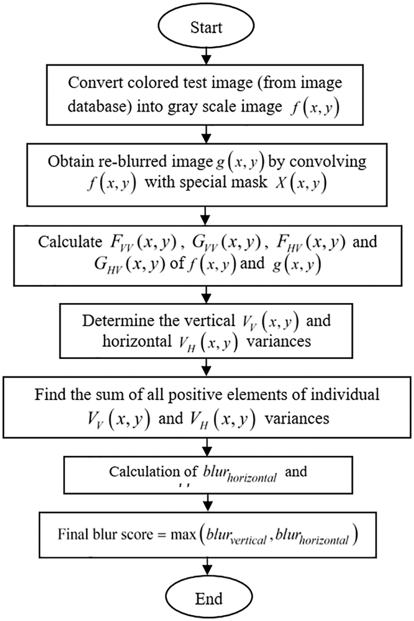
Figure 1: Flow chart of proposed no-reference blur detection algorithm

Step 1: The colored blurred test image of dimensions M × N × 3 is converted into gray scale image f(x, y) of dimensions M × N.

Step 2: The gray scale image is re-blurred with a special mask X(x, y) as given in Eq. (10). Using the convolution method, the re-blurred version g(x, y) of the blurred test image is obtained.

Step 3: The FVV(x, y) and GVV(x, y) is known as vertical variance in pixel intensities of f(x, y) and g(x, y) respectively. The vertical variance is calculated by subtracting the two adjacent columns of the image. Horizontal variance FHV(x, y) and GHV(x, y), on the other hand, are computed by subtracting the pixel intensities of the two adjacent rows of the f(x, y) and g(x, y) respectively.

Step 4: The difference between the test image's pixel-to-pixel variance and the re-blurred image's pixel-to-pixel variance is used to determine the vertical VV(x, y) and horizontal VH(x, y) variances given as follows:

VV(x,y)=FVV(x,y)−GVV(x,y)

VH(x,y)=FHV(x,y)−GHV(x,y)

Step 5: The sum of all the elements of individual vertical VV(x, y) and horizontal VH(x, y) variance whose horizontal and vertical blur variance should be greater than zero.

sumvertical_variance=sum_all_elements_of_VV(x,y)>0

sumhorizontal_variance=sum_all_elements_of_VH(x,y)>0

Step 6: The final horizontal and vertical blur score from the test and re-blurred image is calculated by using following method:

blurvertical=sum_all_elements_of_FVV(x,y)−sumvertical_variancesum_all_elements_of_FVV(x,y)

blurhorizontal=sum_all_elements_of_FHV(x,y)−sumhorizontal_variancesum_all_elements_of_FHV(x,y)

Step 7: The maximum value between the horizontal and vertical blur score is considered as the final blur score.

Final blur score=max(blurvertical,blurhorizontal)

The above algorithm is used to determine the blur score. The objective scores are produced by executing the proposed algorithm on several image datasets. Finally, performance analysis was conducted in terms of various performance parameters using objective and subjective scores.

4  Image Databases and Performance Parameters

Images from publicly available databases LIVE database [44] and TID2013 database [45] are utilized to evaluate the proposed method's performance. The Gaussian blurred images of these databases have been taken to perform the evaluation. The two sample images img66.bmp and img56.bmp are taken from Gaussian blurred images (colored) of LIVE database as shown in Figs. 2b and 2f. The original images of sample images, are shown in Figs. 2a and 2e respectively. Gaussian blurred grayscale and re-blurred images of these images are shown in Figs. 2c–2d and 2g–2h. Similarly, two sample images I05_3.bmp and I21_2.bmp from TID 2013 database. Their original, Gaussian blurred (colored), Gaussian blurred (Grayscale) and re-blurred images are shown in Figs. 2i–2p respectively.

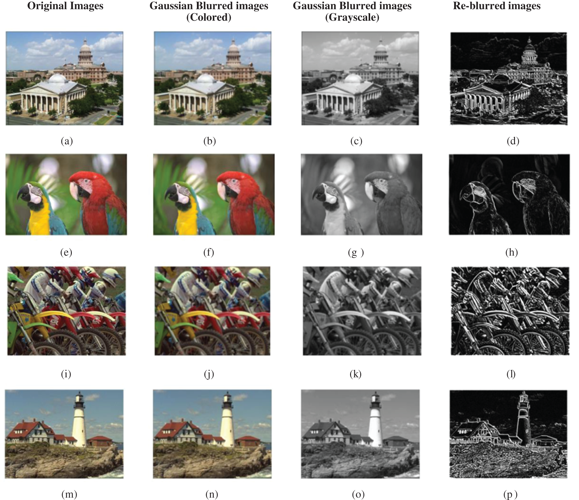
Figure 2: Original, Blurred images in grayscale and re-blurred Images of Gaussian Blurred Images (colored) (b) img66.bmp (634 ×505) (f) img56.bmp (768 ×512) from LIVE Database and (j) I05_3.bmp (512 ×384) (n) I21_2.bmp (512 ×384) from TID 2013 Database respectively

The regression analysis provided by the Video Quality Expert Group (VQEG) [46] was applied on several image databases to evaluate the performance of no-reference blur detection methods [47–49]. Based on this report, some standard performance parameters PLCC,SROCC, MAE, RMSE and OR of no-reference blur assessment algorithm are calculated. To evaluate the performance of no reference blur detection method based on objective scores x and the subjective scores y of various databases, the procedure of VQEG report [46] is followed by many authors [47–49]. Firstly, the Predicted Mean Opinion Scores (MOSP) are calculated based on a logistic function. This function has four model parameters β1, β2, β3, β4 to reduce the sum squared error between the Predicted Mean Opinion Scores (MOSP) and Mean Opinion Scores (MOS) or Differential Mean Opinion Scores (DMOS). The mathematical expression of this function is given below:

MOSP=β1−β21+ex−β3abs(β4)+β2 (11)

Consider the array x = [x1, x2, x3, x4…….xN] are the subjective scores of the database which are already given within the database and y = [y1, y2, y3, y4…….yN] are the evaluated objective scores of the database. The expression for calculation of PLCC is given by the relation:

PLCC=∑i=1N(xi−x¯)(yi−y¯)∑i=1N(xi−x¯)2∑i=1N(yi−y¯)2 (12)

where i = 1, 2, 3, 4……..N are the image numbers of the database images.

SROCC stands for stochastic rank-based correlation approach and it is used to compare two datasets statistically. SROCC coefficient is determined from the mapped subjective scores that is MOS and mapped objective scores that is MOSP. Consider u is the mapping function of the subjective and objective scores, p are mapped objective scores and the q are mapped subjective scores in terms of mapping function, then SROCC can be calculated by using formula:

SROCC=∑i=1N(pi−p¯)(qi−q¯)∑i=1N(pi−p¯)2∑i=1N(qi−q¯)2 (13)

The RMSE is a mathematical grading rule that determines the error's average magnitude. The MAE is a statistic that quantifies the average magnitude of errors in a group of predictions without taking into account their orientation. The MAE and the RMSE can be combined to detect variance in prediction errors. The RMSE will always be greater than or equal to the MAE; the bigger the gap between them, the more variation in the sample's individual errors. The MAE and the RMSE can both be anywhere between 0 to ∞. Root mean square error and mean absolute error can also be determined from the subjective and objective scores according to the mathematical expression given below:

RMSE=∑i=1N(xi−yi)2N (14)

MAE=∑i=1N|xi−yi| (15)

The performance of the blur metric can also be assessed by the outliers ratio. The ratio of false scores obtained by the objective metric to the total scores is known as outliers ratio. The false scores are the outside interval scores dependent on the standard deviation given by [MOS + 2σ, MOS − 2σ], outlier ratio can be calculated as:

OR=FalsescoresTotalscores (16)

Many researchers accepted the non-linear regression analysis for the performance analysis, because it uses the monotonic curve to map the predicted MOS scores with MOS scores, despite the both have different values. The predicted MOS scores are further used for the objective image quality assessment.

4.1 Performance Analysis Using LIVE (Gaussian Blurred) Image Database

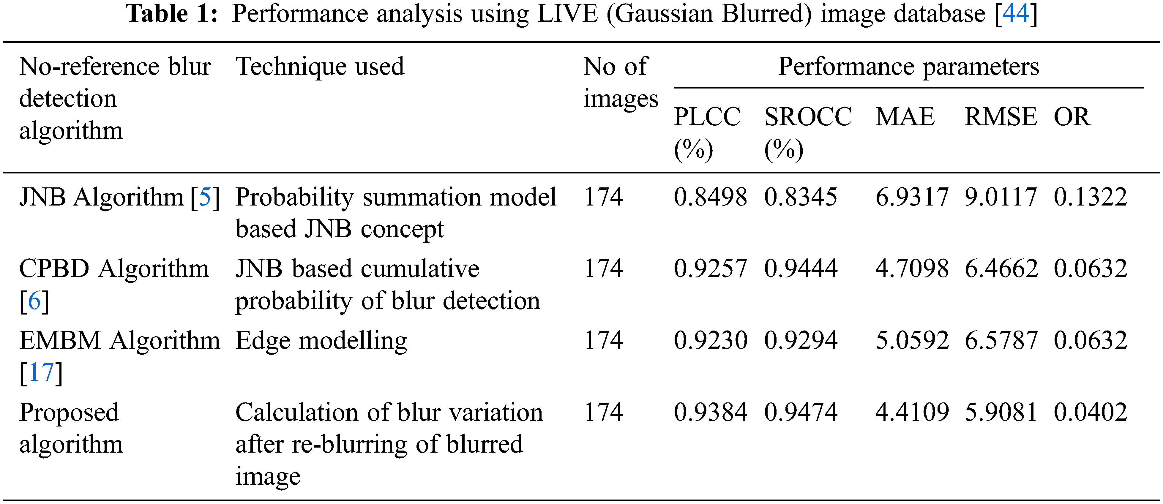
The mathematical model function given in Eq. (11) is used to map objective scores of LIVE database to MOSP of proposed algorithm. The MOSP is calculated from model parameter values β1, β2, β3, β4 which are obtained from the best fit of subjective MOS score. From the MOSP values, the performance parameters of the proposed no-reference blur detection algorithm are calculated. The performance analysis of proposed and existing algorithms for Gaussian blurred images from the LIVE database is presented in Tab. 1. In results, the parameters PLCC is representing prediction accuracy, SROCC is representing prediction monotonicity, MAE and RMSE are representing prediction errors. The OR indicates for the total number of incorrect scores assigned by the objective scores. It is cleared from Tab. 1 that the proposed algorithm outperforms as compared to existing algorithms. The values of PLCC and SROCC obtained maximum which are 0.9384 and 0.9474 respectively, it indicates the objective scores are more accurate. The obtained values of RMSE and MAE are 5.0981 and 4.4109 respectively, which shows the minimum error is obtained in case of proposed algorithm. The minimum value of OR is 0.0402, indicates that incorrect scores obtained are lesser for proposed algorithm as compared to existing algorithms.

Figs. 3a─3d presents the scatter plots of objective scores of proposed and existing algorithms that is JNB [5], CPBD [6] and EMBM [17] against the subjective scores of LIVE database images. The nonlinearity in the mapping of objective scores have been shown by curves of scatter plots. The scatter plot of the proposed algorithm is in opposite direction as compared to existing algorithms for the LIVE database. The curve in Figs. 3a shows the monotonically increasing behavior of objective scores against their respective subjective scores indicates that the proposed algorithm determines the blur from blurred image more precisely as compared to existing algorithms.

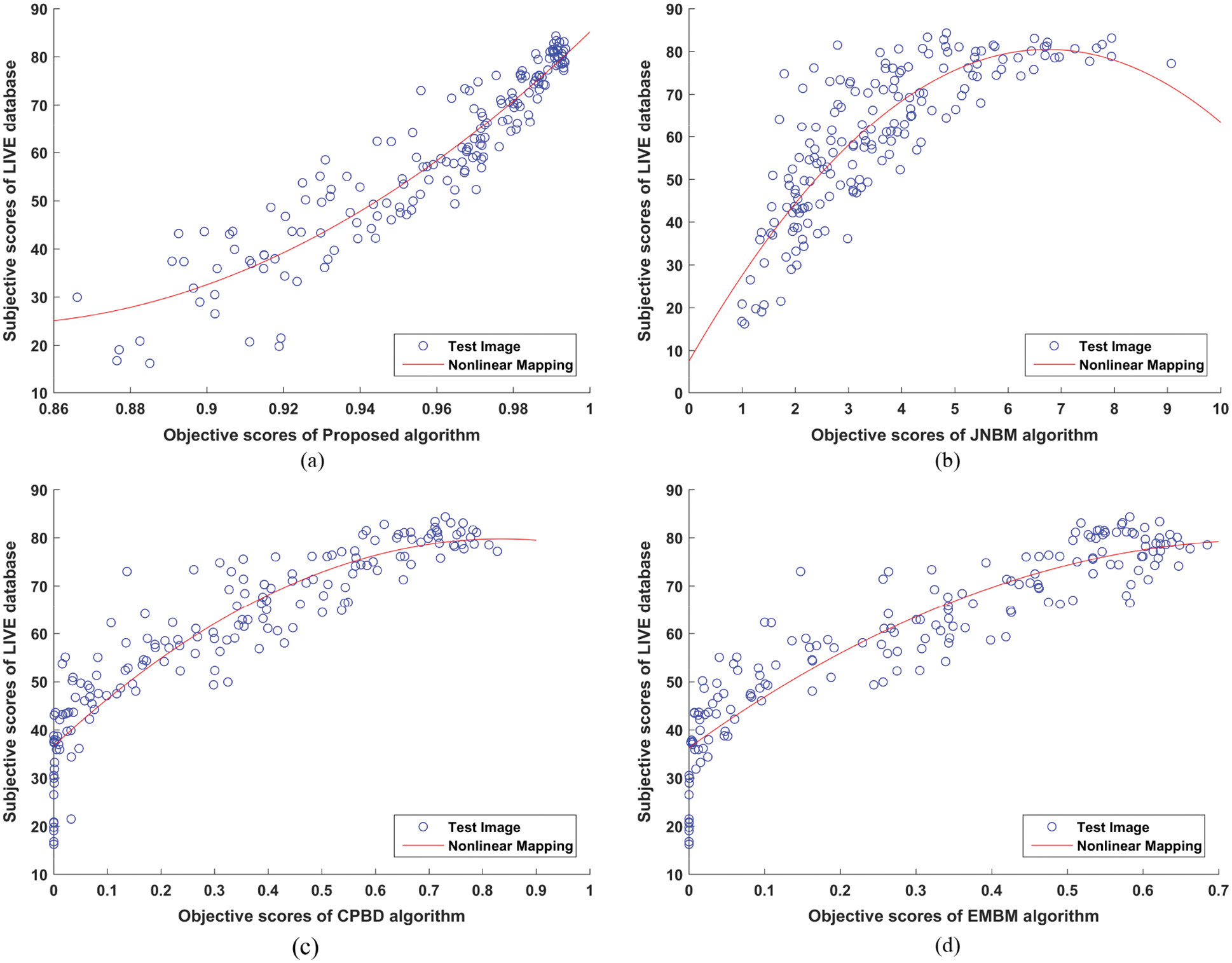
Figure 3: Scatter Plot of Subjective Scores of LIVE Database vs. Objective Scores of (a) Proposed algorithm (b) JNBM algorithm [5] (c) CPBD algorithm [6] (d) EMBM algorithm [17]

4.2 Performance Analysis Using TID2013 (Gaussian Blurred) Image Database

Similarly, for TID2013 database, the MOSP are calculated according to the mathematical model defined by Eq. (11). The MOSP is calculated from model parameter values β1, β2, β3, β4. The performance parameters of the proposed no-reference blur detection algorithm are evaluated using the values of MOSP. For Gaussian blurred images of TID2013 database, performance analysis of proposed and existing algorithms is shown in Tab. 2. It is cleared from the Tab. 2 that the proposed algorithm gives comparative results to EMBM [17] algorithm, but it performs better as compared to JNB [5] and CPBD [6] algorithms. The values of PLCC and SROCC are obtained maximum which are 0.8773 and 0.8664 respectively. The least value obtained by RMSE is 0.5989. The obtained values of MAE and OR are 4.4862 and 0.6880. The resulting parameter values indicate that objective scores are more accurate, with a lower rate of false scores and error.

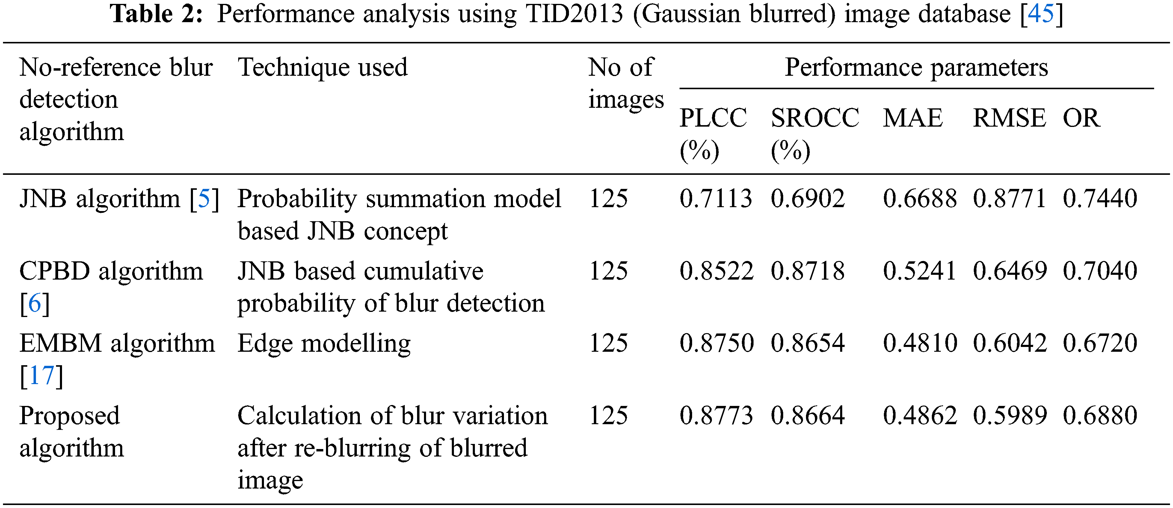
Fig. 4a─4d presents the scatter plots of objective scores of proposed and existing algorithms that is JNB [5], CPBD [6] and EMBM [17] against the subjective scores of TID 2013 database. The scatter plot curve in Fig. 4a shows the nonlinearity in the mapping of objective scores. When compared to existing algorithms, the scatter plot of the proposed algorithm for TID 2013 is also in the opposite direction, but shows the monotonically increasing behavior of objective scores against their respective subjective scores for proposed and existing algorithms. When compared to existing methods, the proposed algorithm performs very well for Gaussian blurred images from the LIVE database, but it is identical to the EMBM method for the Gaussian blurred images of TID 2013 database.

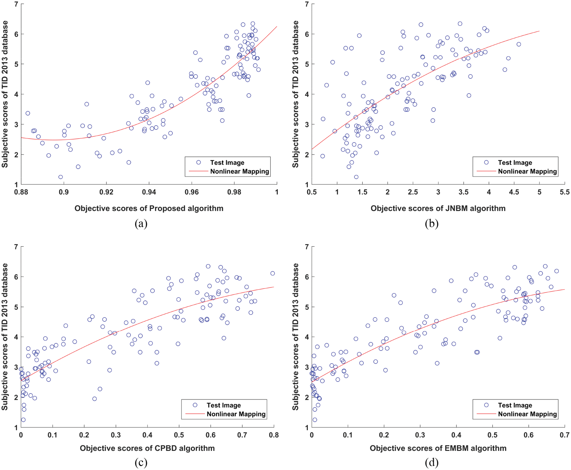
Figure 4: Scatter Plot of Subjective Scores of TID2013 Database vs. Objective Scores of (a) Proposed algorithm (b) JNBM algorithm [5] (c) CPBD algorithm [6] (d) EMBM algorithm [17]

5  Conclusion

Using the re-blurring concept, we were able to deal with the problem of no-reference image blur assessment. The goal of this re-blurring concept is to get beyond the limitations of earlier no-reference blur assessment algorithms. Unlike earlier research, the proposed technique does not rely on edge detection or block processing to calculate blur in a no-reference image. Instead, it relies on the variation of pixel intensities after re-blurring of image. The computation of the blur score has been done using a two-step process. The Laplace filter has been used to create a Markov-based special mask in the first step. In the next step, the blurred image was re-blurred using this special mask and pixel intensity variations were calculated. The final blur score was calculated using the highest value of blur score from both the horizontal and vertical blur scores. To demonstrate the usefulness of the proposed algorithm, Gaussian blurred images from the LIVE and TID 2013 databases were utilized. The results illustrate that the proposed method was successful in predicting high blur scores with high accuracy as compared to existing no-reference blur assessment algorithms such as JNB, CPBD and EMBM algorithms. The future scope of research included that this method can also be improved by using optimization techniques in the selection of special mask. The work can be further extended by using genetic algorithms and machine learning concepts.

Funding Statement: The authors received no specific funding for this study.

Conflicts of Interest: The authors declare that they have no conflicts of interest to report regarding the present study.

References

 1.  A. Zaric, M. Loncaric, D. Tralic, M. Brzica, E. Dumic et al., “Image quality assessment-comparison of objective and subjective measures with results of subjective test,” in 52nd Int. Symp. ELMAR 2010, Zadar, Croatia, pp. 113–118, 2010. [Google Scholar]

 2.  S. Gabarda, G. Cristobal and N. Goel, “Anisotropic blind image quality assessment: Survey and analysis with current methods,” Journal of Visual Communication and Image Representation, vol. 52, pp. 101–105, 2018. [Google Scholar]

 3.  E. Cohen and Y. Yitzhaky, “No-reference assessment of blur and noise impacts on image quality,” Springer, London, vol. 4, no. 3, pp. 289–302, 2010. [Google Scholar]

 4.  P. Marziliano, F. Dufaux, S. Winkler and T. Ebrahimi, “Perceptual blur and ringing metrics: Application to JPEG2000,” Signal Processing: Image Communication, vol. 19, pp. 163–172, 2004. [Google Scholar]

 5.  R. Ferzli and L. J. Karam, “A no-reference objective image sharpness metric based on the notion of just noticeable blur (JNB),” IEEE Transactions on Image Processing, vol. 18, no. 4, pp. 717–728, 2009. [Google Scholar]

 6.  N. D. Narvekar and L. J. Karam, “A no-reference image blur metric based on the cumulative probability of blur detection (CPBD),” IEEE Transactions on Image Processing, vol. 20, no. 9, pp. 2678–2681, 2011. [Google Scholar]

 7.  F. Kerouh and A. Serir, “A perceptual blind blur image quality metric,” in Proc. ICASS, IEEE Int. Conf. on Acoustics, Speech and Signal Processing, Florence, Italy, pp. 2784–2788, 2014. [Google Scholar]

 8.  S. Wu, W. Lin, L. Jiang, W. Xiong and L. Chen, “An objective out-of-focus blur measurement,” in Proc. ICICSP, IEEE Int. Conf. on Information Communications and Signal Processing, Bangkok, Thailand, pp. 334–338, 2005. [Google Scholar]

 9.  D. B. Bong and A. S. Ng, “Full-reference and no-reference image blur assessment based on edge information,” International Journal on Advanced Science Engineering Information Technology, vol. 2, no. 1, pp. 90–95, 2012. [Google Scholar]

10. Y. Wang, H. Du, J. Xu and Y. Liu, “A No-reference perceptual blur metric based on complex edge analysis,” in Proc. IC-NIDC, 3rd IEEE, Int. Conf. on Network Infrastructure and Digital Content, Beijing, China, pp. 487–491, 2012. [Google Scholar]

11. K. Bahrami and A. C. Kot, “A fast approach for no-reference image sharpness assessment based on maximum local variation,” IEEE Signal Process Letters, vol. 21, pp. 751–755, 2014. [Google Scholar]

12. S. Wang, C. Deng, B. Zhao, G. B. Huang and B. Wang, “Gradient based No-reference image blur assessment using extreme learning machine,” Journal of Neurocomputing, Elsevier, vol. 174, part A, 22, pp. 310–321, 2016. [Google Scholar]

13. L. Liang, J. Chen, S. Ma, D. Zhao and W. Gao, “A no-reference perceptual blur metric using histogram of gradient profile sharpness,” in Proc. ICIP, IEEE, Int. Conf. on Image Processing, Cairo, Egypt, pp. 4369–4372, 2009. [Google Scholar]

14. Z. Li, Y. Liu, J. Xu and H. Du, “A no-reference perceptual blur metric based on the blur ratio of detected edges,” in Proc. IC-BNMT, 5th IEEE, Int. Conf. on Broadband Network and Multimedia Technology, Guilin, China, pp. 1–5, 2013. [Google Scholar]

15. S. Ezekiel, K. Harrity, E. Blasch and A. Bubalo, “No-reference blur metric using double-density and dual-tree two-dimensional wavelet transformation,” in Proc. NAECON, IEEE National Aerospace and Electronics Conf., Dayton, OH, USA, pp. 109–114, 2014. [Google Scholar]

16. F. Kerouh and A. Serir, “A no reference perceptual blur quality metric in DCT domain,” in Proc. ICCEIT, IEEE, Int. Conf. on Control Engineering and Information Technology, Tlemcen, Algeria, pp. 1–6, 2015. [Google Scholar]

17. J. Guan, W. Zhang, J. Gu and H. Ren, “No-reference blur assessment based on edge modeling,” Journal of Visual Communication and Image Representation, vol. 29, pp. 1–7, 2015. [Google Scholar]

18. L. Platisa, A. Pizurica, E. Vasteenkiste and W. Philips, “Image blur assessment based on the average cone ratio in the wavelet domain,” in Proc. Int. Conf. on Wavelet Applications in Industrial Processing VI, SPIE, the Int. Society for Optical Engineering, San Jose, California, United States, vol. 7248, pp. 1–10, 2009. [Google Scholar]

19. E. Mavridaki and V. Mezaris, “No-reference blur assessment in natural images using Fourier transform and spatial pyramids,” in Proc. ICIP, IEEE, Int. Conf. on Image Processing, Paris, France, pp. 566–570, 2014. [Google Scholar]

20. S. Ezekiel, K. Harrity, M. Alford, E. Blasch, D. Farris et al., “No-reference objective blur metric based on the notion of wavelet gradient, magnitude width,” in Proc. NAECON, IEEE, National Aerospace and Electronics Conf., Dayton, OH, USA, pp. 115–120, 2014. [Google Scholar]

21. C. Lu, “No-reference image blur measurement based on wavelet high frequency domain analysis,” in Proc. ICISE, IEEE, Int. Conf. on Information Science and Engineering, Hangzhou, China, pp. 3844–3846, 2010. [Google Scholar]

22. S. Yousaf and S. Qin, “Approach to metric and discrimination of blur based on its invariant features,” in Proc. ICIST, IEEE, Conf. on Imaging Systems and Techniques, Beijing, China, pp. 274–279, 2013. [Google Scholar]

23. D. Liu, Z. Chen, H. Ma, F. Xu and X. Gu, “No reference block based blur detection,” in Proc. IEEE, Int. Workshop on Quality of Multimedia Experience, San Diego, CA, USA, pp. 75–80, 2009. [Google Scholar]

24. R. Hassan, Z. Wang and M. Salama, “Image sharpness assessment based on local phase coherence,” IEEE Transactions on Image Processing, vol. 22, no. 7, pp. 2798–2810, 2013. [Google Scholar]

25. P. V. Vu and D. M. Chandler, “A fast wavelet-based algorithm for global and local image sharpness estimation,” IEEE Signal Processing Letters, vol. 19, no. 7, pp. 423–426, 2012. [Google Scholar]

26. Q. Sang, H. Qi, X. Wu, C. Li and A. C. Bovik, “No-reference image blur index based on singular value curve,” Journal of Visual Communication and Image Representation, vol. 25, no.7, pp. 1625–1630, 2014. [Google Scholar]

27. X. Fang, F. Shen, Y. Guo, C. Jacquemin, J. Zhou et al., “A consistent pixel-wise blur measure for partially blurred images,” in Proc. ICIP, IEEE, Int. Conf. on Image Processing, Paris, France, pp. 496–500, 2014. [Google Scholar]

28. K. Harrity, S. Ezekiel, M. Ferris, M. Comacchia and E. Blasch, “No-reference multi-scale blur metric,” in Proc. NAECON, IEEE, National Aerospace and Electronics Conf., Dayton, OH, USA, pp. 103–108, 2014. [Google Scholar]

29. F. Crété-Roffet, T. Dolmiere, P. Ladret and M. Nicolas, “The blur effect: Perception and estimation with a new no-reference perceptual blur metric,” in Proc. SPIE, Electronic Imaging Symp. Conf. on Human Vision and Electronic Imaging, San Jose, CA, United States, vol. 12, pp. EI-6492, 2007. [Google Scholar]

30. A. Chetouani, A. Beghdadi and M. Deriche, “A new reference-free image quality index for blur estimation in frequency domain,” in IEEE Int. Symp. on Signal Processing and Information Technology (ISSPIT), Ajman, United Arab Emirates, pp. 155–159, 2009. [Google Scholar]

31. D. B. Bong and B. E. Khoo, “An efficient and training-free blind image blur assessment in the spatial domain,” IEICE Transactions on Information and Systems, vol. 97, no. 7, pp. 1864–1871, 2014. [Google Scholar]

32. D. B. L. Bong and B. E. Khoo, “Blind image blur assessment by using valid reblur range and histogram shape difference,” Signal Processing: Image Communication, vol. 29, no. 6, pp. 699–710, 2014. [Google Scholar]

33. E. Kalalembang, K. Usman and I. P. Gunawan, “DCT-Based local motion blur detection,” in Proc. ICIC-BME, IEEE, Int. Conf. on Instrumentation, Communications Information Technology and Biomedical Engineering, Bandung, Indonesia, pp. 1–6, 2009. [Google Scholar]

34. R. Dosselmann and X. D. Yang, “No-reference noise and blur detection via the Fourier transform,” Dept. of Computer Science, Univ. of Regina. Regina, SK (Saskatchewan), Canada, August, 2012. [Google Scholar]

35. K. Gu, J. Zhou, J. F. Qiao, G. Zhai, W. Lin et al., “No-reference quality assessment of screen content pictures,” IEEE Transactions on Image Processing, vol. 26, no. 8, pp. 4005–4018, 2017. [Google Scholar]

36. W. Zhou, L. Yu, W. Qiu, Y. Zhou and M. Wu, “Local gradient patterns (LGPAn effective local-statistical-feature extraction scheme for no-reference image quality assessment,” Information Sciences, vol. 397, pp. 1–14, 2017. [Google Scholar]

37. X. Chen, Q. Zhang, M. Lin, G. Yang and C. He, “No-reference color image quality assessment: From entropy to perceptual quality,” EURASIP Journal on Image and Video Processing, vol. 1, pp. 1–14, 2019. [Google Scholar]

38. C. Sun, Z. Cui, Z. Gan and F. Liu, “No-reference image blur assessment based on multi-scale spatial local features,” KSII Transactions on Internet and Information Systems (TIIS), vol. 14, no. 10, pp. 4060–4079, 2020. [Google Scholar]

39. D. Li, T. Jiang and M. Jiang, “Exploiting high-level semantics for no-reference image quality assessment of realistic blur images,” in Proc. 25th ACM Int. Conf. on Multimedia, New York, NY, United States, pp. 378–386, 2017. [Google Scholar]

40. C. Yan, T. Teng, Y. Liu, Y. Zhang, H. Wang et al., “Precise no-reference image quality evaluation based on distortion identification,” ACM Transactions on Multimedia Computing, Communications and Applications (TOMM), vol. 17, no. 3s, pp. 1–21, 2021. [Google Scholar]

41. H. Zhu, L. Li, J. Wu, W. Dong and G. Shi, “MetaIQA: Deep meta-learning for no-reference image quality assessment,” in Proc. IEEE/CVF Conf. on Computer Vision and Pattern Recognition, Seattle, WA, USA, pp. 14143–14152, 2020. [Google Scholar]

42. S. Aoki and A. Takemura, “The largest group of invariance for markov bases and toric ideals,” Journal of Symbolic Computation, vol. 43, no. 5, pp. 342–358, 2008. [Google Scholar]

43. A. Takemura and S. Aoki, “Some characterizations of minimal markov basis for sampling from discrete conditional distributions,” Annals of the Institute of Statistical Mathematics, vol. 56, no. 1, pp. 1–17, 2004. [Google Scholar]

44. H. R. Sheikh, Z. Wang, L. Cormack and A. C. Bovik, “LIVE image quality assessment database release 2,” [Online]. Available: http://live.ece.utexas.edu/research/quality, 2005. [Google Scholar]

45. N. Ponomarenko, L. Jin, O. Ieremeiev, V. Lukin, K. Egiazarian et al., “Image database TID2013: Peculiarities, results and perspectives,” Signal Processing: Image Communication, vol. 30, pp. 57–77, 2015. [Google Scholar]

46. J. Antkowiak, T. J. Baina, F. V. Baroncini, N. Chateau, F. FranceTelecom et al., Final report from the Video Quality Experts group on the validation of objective models of Video Quality assessment. Technical report, 2000, http://www.vqeg.org. [Google Scholar]

47. K. Gu, G. Zhai, X. Yang and W. Zhang, “Hybrid no-reference quality metric for singly and multiply distorted images,” IEEE Transactions on Broadcasting, vol. 60, no. 3, pp. 557–567, 2014. [Google Scholar]

48. L. Cui and A. R. Allen, “An image quality metric based on corner, edge and symmetry maps,” in Proc. BMVC, British Machine Vision Conf., Leeds, UK, pp. 1–10, 2008. [Google Scholar]

49. H. R. Sheikh and A. C. Bovik, “Image information and video quality,” IEEE Transactions on Image Processing, vol. 15, no. 2, pp. 430–444, 2006. [Google Scholar]

This work is licensed under a Creative Commons Attribution 4.0 International License, which permits unrestricted use, distribution, and reproduction in any medium, provided the original work is properly cited.