DOI:10.32604/iasc.2023.025968
| Intelligent Automation & Soft Computing DOI:10.32604/iasc.2023.025968 | |
| Article |
Deep Learning Enabled Financial Crisis Prediction Model for Small-Medium Sized Industries
SSN School of Management, Kalavakkam, Chennai, 603110, India
*Corresponding Author: Kavitha Muthukumaran. Email: mkavitha@ssn.edu.in
Received: 10 December 2021; Accepted: 27 February 2022
Abstract: Recently, data science techniques utilize artificial intelligence (AI) techniques who start and run small and medium-sized enterprises (SMEs) to take an influence and grow their businesses. For SMEs, owing to the inexistence of consistent data and other features, evaluating credit risks is difficult and costly. On the other hand, it becomes necessary to design efficient models for predicting business failures or financial crises of SMEs. Various data classification approaches for financial crisis prediction (FCP) have been presented for predicting the financial status of the organization by the use of past data. A major process involved in the design of FCP is the choice of required features for enhanced classifier outcomes. With this motivation, this paper focuses on the design of an optimal deep learning-based financial crisis prediction (ODL-FCP) model for SMEs. The proposed ODL-FCP technique incorporates two phases: Archimedes optimization algorithm based feature selection (AOA-FS) algorithm and optimal deep convolution neural network with long short term memory (CNN-LSTM) based data classification. The ODL-FCP technique involves a sailfish optimization (SFO) algorithm for the hyperparameter optimization of the CNN-LSTM method. The performance validation of the ODL-FCP technique takes place using a benchmark financial dataset and the outcomes are inspected in terms of various metrics. The experimental results highlighted that the proposed ODL-FCP technique has outperformed the other techniques.
Keywords: Small medium-sized enterprises; deep learning; FCP; financial sector; prediction; metaheuristics; sailfish optimization
In recent times, there has been an increase in the financial crisis of companies all over the world, they are giving considerable attention to the field of financial crisis prediction (FCP) [1]. For a financial institution /company, it is highly needed to develop a consistent and early predictive method to predict the possible risks of the company status of earlier financial risk. Commonly FCP produces a binary classification method that has been resolved efficiently [2]. The outcomes from the classification method are classified as follows: failure and non-failure status of a company [3]. So far, several classification methods have been designed by a large number of domain knowledge for FCP. In general, the proposed method is separated into artificial intelligence (AI) /statistical methodologies.
The precision of the FCP plays a significant role to define the financial firms’ profitability and productivity [4]. For instance, a small positive adjustment from the accuracy levels of a promising customer with default credit would minimalize a great future loss of organizations [5]. FCP is considered as a data classification problem, that represents the user as “default” or user is represented as “non-default” once they return the loan. Several studies have been conducted on the FCP classification, starting at the beginning of the year 1960′s. In recent times, conventional approaches applied numerical function to forecast financial crisis that differentiates financial institutions from weaker and stronger ones [6]. During 1990’s, the focus has moved towards machine learning (ML) and artificial intelligence (AI) based expert systems such as Support Vector Machines (SVM) and Neural Network (NN). Lately, AI methods are adapted to improve the traditional classification methods. But, the existence of various characteristics in the higher-dimension financial data results in various problems such as low interoperability, overfitting, and high computational complexity [7]. The convenient method to resolve this problem is decreasing the available amount of features with feature selection (FS) methods [8].
The FS method is one of the vital and effective pre-processing phases in Data Mining (DM). It is accountable to extract the redundant and unwanted features from original information [9]. Furthermore, it is employed to extract high possible data through minimal feature subset and potential characteristics such as computation time, noise elimination, minimizing of impure feature, and reduced cost that is crucial to implement an approximation method [10]. Moreover, FS is applied to process the feature subset under the applications of fixed value instead of utilizing elected features. The key challenge in this method is detecting optimum features from available features called NP-hard problems [11]. Various methods are employed to identify partial solutions using shorter time intervals. Certain ML techniques such as gray wolf optimizer (GWO), particle swarm optimization (PSO), and ant colony optimization (ACO) are employed in choosing crucial features, however, such methods aren’t relevant in the business application, mainly in FCP.
This paper presents an optimal deep learning based FCP (ODL-FCP) model for SMEs. The major aim of the ODL-FCP technique is to determine the financial status of SMEs. The proposed ODL-FCP technique contains the design of the Archimedes optimization algorithm based feature selection (AOA-FS) algorithm to derive optimal feature subset. In addition, the sailfish optimization (SFO) algorithm with a convolution neural network with long short term memory (CNN-LSTM) is utilized for data classification. To showcase the enhanced classification efficiency of the ODL-FCP technique, a wide range of simulations were carried out against benchmark financial datasets and the outcomes are examined concerning various metrics.
Uthayakumar et al. [12] presented an ant colony optimization (ACO) based FCP method that integrates 2 phases: ant colony optimization based feature selection (ACO-FS) and ant colony optimization based data classification (ACO-DC) algorithms. The presented method is confirmed by a group of 5 standard datasets including quantitative and qualitative. For the FS model, the presented ACO-FS technique is compared to 3 current FCP techniques algorithms. Yan et al. [13] developed a new method of DL prediction, according to that, create a DL hybrid predictive method for stock markets—complementary ensemble empirical mode decomposition principal component analysis long term short memory (CEEMD-PCA-LSTM). During this method, CEEMD, as an order smoothing and decomposition model, capable of decomposing the trends/fluctuations of distinct scales of time sequence gradually, generates a sequence of intrinsic mode function (IMF) using distinct characteristic scale. Next, a higher-level abstract feature is individually fed into the LSTM network for predicting the final price of the trading for all the components.
Yang [14] presented a method-based DL architecture for predicting the financial indicator value. The presented method applies the LSTM method as a standard predictive method. This architecture estimates the economic condition to define the number of financial failures to the organization and warns of any fluctuation in the forecasted 3 indicator values. Perboli et al. [15] aimed at mid-and long-term bankruptcy prediction (up to sixty months) targeting smaller/medium enterprises. Samitas et al. [16] examined on “Early Warning System” (EWS) by examining potential contagion risk, according to structured financial network. The presented method improves typical crisis predictive model performances. With machine learning algorithms and network analysis, they detect proof of contagion risks on the date where they witness considerable raise in centralities and correlations.
Uthayakumar et al. [17] introduced a cluster-based classification method that includes: fitness-scaling chaotic genetic ant colony algorithm (FSCGACA) based classification method and enhanced K-means clustering. Initially, an enhanced K-means method is developed to remove the incorrectly clustered information. Next, a rule-based method is chosen for fitting the provided dataset. Finally, FSCGACA is utilized to search for the best possible parameter of the rule-based method. Tyagi et al. [18] presented a smart Internet of Things (IoT) assisted FCP method with Meta-heuristic models. The presented FCP model contains classification, data acquisition, pre-processing, and FS. Initially, the financial information of the organization is gathered by IoT gadgets like laptops, smartphones, and so on. Then, the quantum artificial butterfly optimization (QABO) method for FS is employed to select optimum sets of features.
In this paper, an efficient ODL-FCP technique has been presented for the identification of the financial crisis of SMEs. The proposed ODL-FCP technique encompasses major sub-processes namely pre-processing, arithmetic optimization algorithm (AOA) based selection of features, CNN-LSTM based classification, and SFO based hyperparameter tuning. The utilization of AOA for the optimal selection of features and SFO for the hyperparameter optimization process aid to accomplish improved classification performance. Fig. 1 demonstrates the overall block diagram of the proposed ODL-FCP technique.
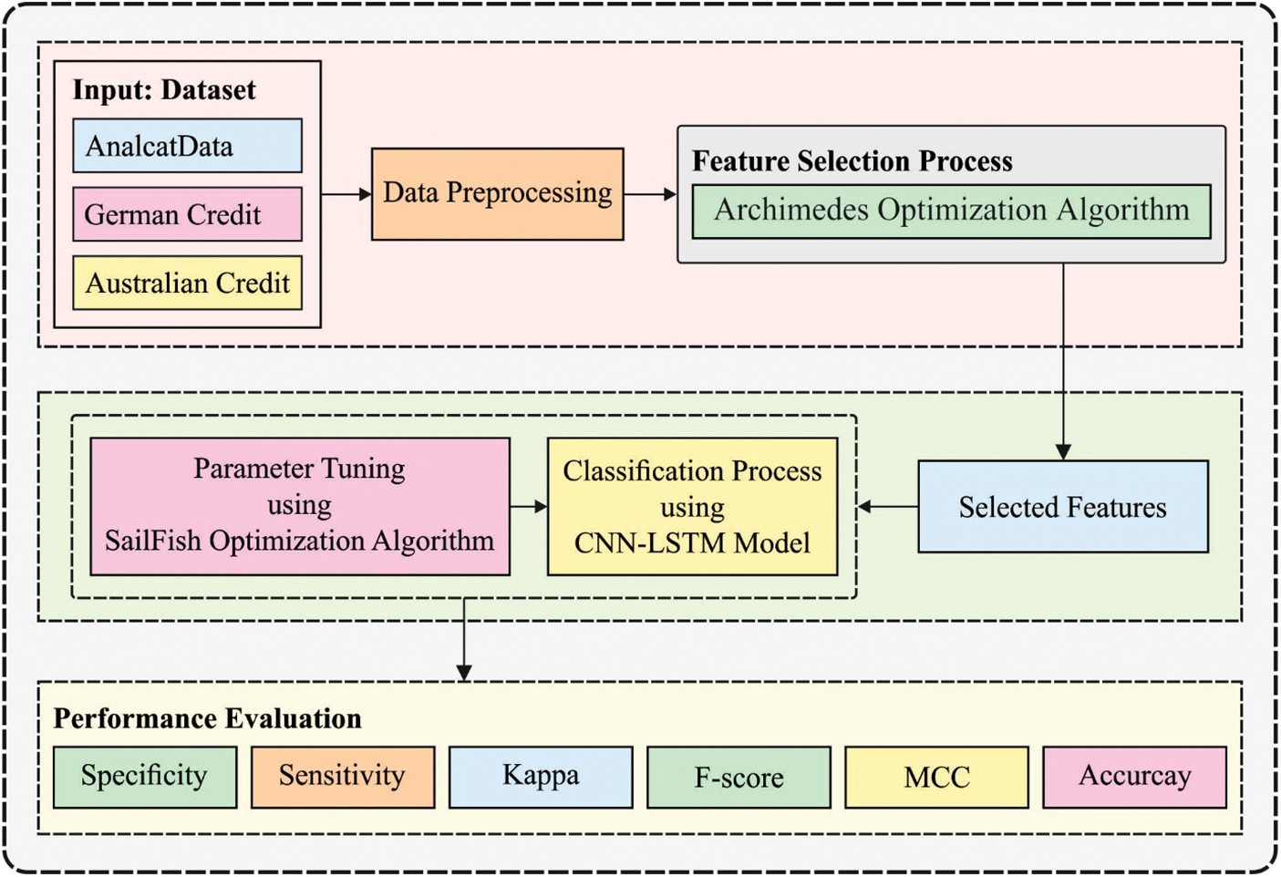
Figure 1: Overall process of proposed framework
The financial data has extremely difficult and is collected of fundamental signals with many distinct features. But determining the transformation performance from cellular network confidently is help for enhancing networks data forecast techniques. For avoiding load packets with superior numeric values from the network in controlling individuals with lesser numeric values, the data is scaled; it also improves the modeling speed of the technique but continues optimum accuracy. A min-max technique is utilized for transforming the data to value amongst [0,1]; scaling the data is used from increasing the model to forecast network traffics. The two important benefits of scaling are for avoiding samples of higher numeric ranges controlling individuals with minimal numeric ranges and for preventing numerical problems under the forecast. The transformation has realized as follows:
where
3.2 Design of AOA-FS Technique
Once the financial data are pre-processed, the appropriate selection of features was carried out using the AOA-FS technique. During this effort, the AOA technique [19] was utilized for solving the presented optimized issue together with NR mathematical technique. The AOA approach is a meta-heuristic technique employed for solving many mathematical optimized issues and is verified their capability for fetching towards a global solution from a short time. The AOA essential condition hinges on Archimedes’ rule of buoyancy. The AOA allows several phases determining a near-global solution, and these phases are demonstrated as:
Phase 1 ‘Initialized’: In this step, the populations containing the immersed object (solution) are considered by its volume, density, and acceleration. All solutions are initialized with an arbitrary place from the fluid as offered in Eq. (2), afterward the fitness value to all solutions is estimated.
where
Phase 2 ‘Upgrade density and volume’: During this phase, the density and volumes of all the solutions were upgraded utilizing the subsequent equations:
where
Phase 3 ‘Transfer operator and density factor’: During this phase, the collision amongst solutions is still in its equilibrium state. The mathematical process of the collision was demonstrated as:
where
Phase 4 ‘Exploration’: During this phase, the collision amongst solution occurs. Therefore, when
where
Phase 5 ‘Exploitation’: During this phase, no collision amongst solution occurs. Therefore, when
where
Phase 6 ‘Normalize acceleration’: The acceleration was normalization for assessing the percentage of the alteration as follows:
where
Phase 7 ‘Evaluation’: The fitness value of all solutions was estimated under this phase, and optimum solutions are registered, for instance, upgrade the optimum solutions
Different from the classical AOA in which the solution was upgraded from the exploring space near the continued valued place from the BAOA, the searching space was demonstrated as
During the binary techniques, one utilizes the step vector for evaluating the possibility of altering place, the transfer function significantly influences the balance amongst exploitation as well as exploration. During the FS technique, once the size of the feature vector demonstrates
According to the aforementioned, the FF for determining solution under this state produced for attaining a balance amongst the 2 objectives as:
3.3 Design of CNN-LSTM Classifier
During the classification process, the CNN-LSTM model gets executed to identify the financial status of the SMEs. The CNN layer extracts the data patterns automatically. The order of features can be learned one more time in the LSTM layer. The presented method constantly tunes hyperparameters based on the outcomes from learning LSTM and CNN. CNN layer extracts parameters that are significant for classification. Especially, this is validated by the class activation maps. Also, the pooling layer reduces the spatial size of feature vectors, reduces the number of variables and computation difficulty of the NN. They could automatically alter hyper parameters like several filters, filter size, and several layers. Eq. (14) signifies the process of
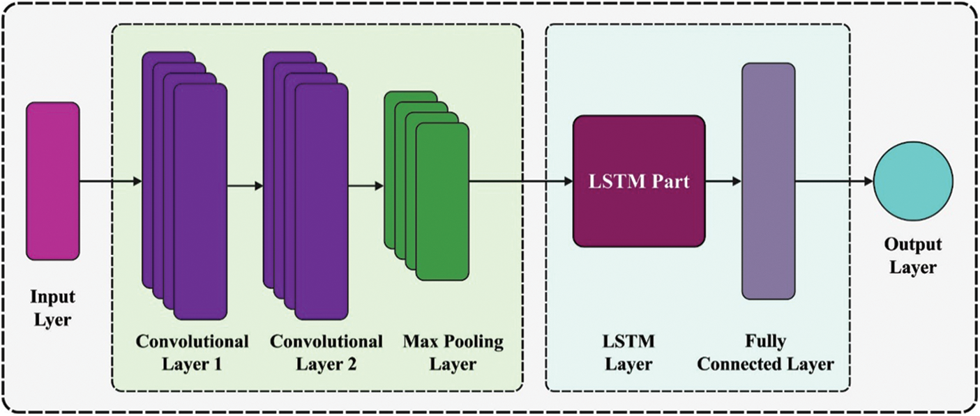
Figure 2: Structure of CNN-LSTM model
To generate a non-linear decision boundary,
The pooling layer is utilized for improving the classifier accuracy of the access control scheme and minimalizing the computational costs. Eq. (16) denotes the pooling layer operation. The pooling layer enables to minimalize over-fitting and effectively extracts features.
LSTM learns temporal data according to the feature extracted from CNN. Eq. (17) indicates the 3 gates state which completes the LSTM process that controls the sequential data of a database query as a constant value among zero and one. Every cell contains forget input and output gates. Eq. (17) is denoted as the resultant value of
Eq. (20) illustrates the FC layer operation. The output of the FC layer is categorized as zero/one by softmax. Eq. (21) evaluates the role classification possibility.
3.4 Hyper Parameter Tuning Using SFO Algorithm
For resolving the limitation of the CNN-LSTM model of trapping into local optima problem at the time of learning and training processes, the SFO algorithm is utilized for optimizing and adjusting the parameters involved in the CNN-LSTM Model and determining the optimum initial weight of the network.
The SFO is a new nature simulated meta-heuristic technique that is demonstrated then a set of hunting sailfish. It depicts competitive efficiency related to famous meta-heuristic techniques. During the SFO technique, it can be considered that sailfish is a candidate solution and which places of sailfish under the search space signify the variables of issue. The place of
where
The variable
where
The variable
where
Initially the hunted, sailfishes are energetic, and sardines aren’t tired/injured. The sardines are escape quickly. But, with continued hunting, the control of sailfish attacks is slowly reduced. In the meantime, the sardines are come to be tired, and their awareness of the place of the sailfish is also reduced. Thus, the outcome, the sardines are hunted. According to the algorithmic procedure, a novel place of sardine
where
The variable
where
where
where
The experimental results analysis of the ODL-FCP technique takes place using three benchmark datasets namely Alancatdata, German Credit, and Australian Credit datasets. The first AnalcatData dataset includes 50 samples under two classes. Next, the second dataset comprises 1000 samples with two classes. The final dataset has 690 samples with two classes. Tab. 1 offers the FS outcome of the AOA-FS technique. The results show that the AOA-FS technique has chosen only a minimal number of features. For instance, the AOA-FS technique has selected a total of 3, 10, and 8 features on the test AnalcatData, German Credit, and Australian Credit datasets respectively.

Fig. 3 demonstrates the best cost (BC) analysis of the AOA-FS technique with other FS models on AnalcatData Dataset. Fig. 3 shows that the AOA-FS technique has resulted ineffectual FS outcomes with minimal BC. For instance, under 3 iterations, the AOA-FS technique has obtained a lower BC of 0.0269 whereas the QABO-FS, ACO-FS, and grey wolf optimization based feature selection (GWO-FS) techniques have attained higher BC of 0.0347, 0.0466, and 0.0715 respectively. At the same time, under 6 iterations, the AOA-FS approach has reached minimal BC of 0.0246 whereas the QABO-FS, ACO-FS, and GWO-FS methods have obtained superior BC of 0.0316, 0.0466, and 0.0607 correspondingly. Moreover, under 9 iterations, the AOA-FS technique has gained a lower BC of 0.0223 whereas the QABO-FS, ACO-FS, and GWO-FS techniques have attained superior BC of 0.0315, 0.0466, and 0.5743 correspondingly.
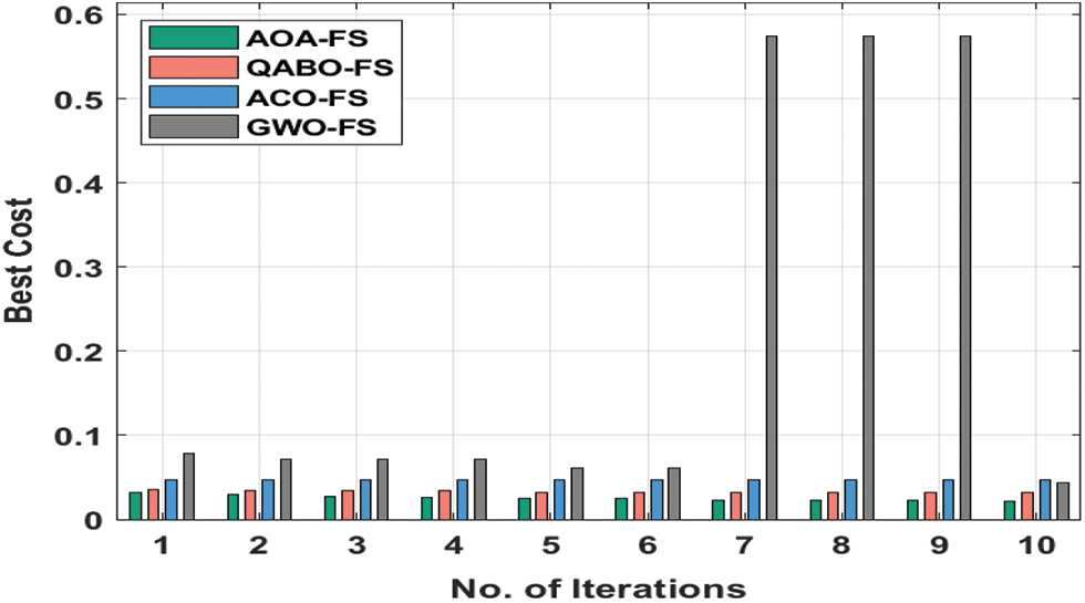
Figure 3: BC analysis of AOA-FS technique on AnalcatData dataset
Fig. 4 determines the BC analysis of the AOA-FS system with other FS manners on the German Credit Dataset. Fig. 4 outperformed that the AOA-FS technique has resulted in effective FS outcome with the minimal BC. For the sample, under 3 iterations, the AOA-FS technique has obtained least BC of 0.1477 but the QABO-FS, ACO-FS, and GWO-FS techniques have achieved superior BC of 0.1532, 0.1600, and 0.1600 correspondingly. Simultaneously, under 6 iterations, the AOA-FS technique has obtained lower BC of 0.1334 whereas the QABO-FS, ACO-FS, and GWO-FS techniques have attained higher BC of 0.1467, 0.1500, and 0.1600 respectively. Also, under 9 iterations, the AOA-FS technique has obtained minimum BC of 0.1099 while the QABO-FS, ACO-FS, and GWO-FS techniques have attained a higher BC of 0.1258, 0.1400, and 0.1600 correspondingly.
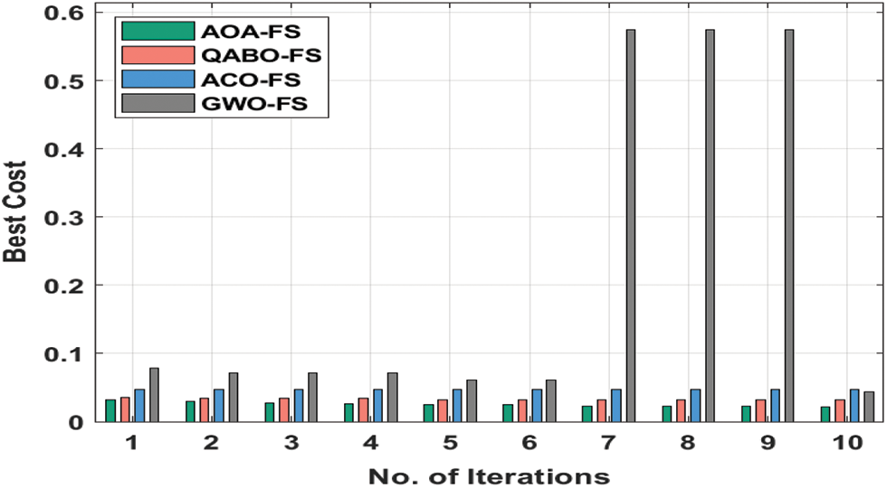
Figure 4: BC analysis of AOA-FS technique on German credit dataset
Fig. 5 reveals the BC analysis of the AOA-FS approach with other FS models on the Australian Credit Dataset. Fig. 5 revealed that the AOA-FS system has resulted in effective FS outcomes with minimal BC. For instance, under 3 iterations, the AOA-FS method has reached a minimum BC of 0.0471 whereas the QABO-FS, ACO-FS, and GWO-FS methods have gained superior BC of 0.0652, 0.0830, and 0.0990 respectively. Followed by, under 6 iterations, the AOA-FS technique has reached a lower BC of 0.0429 whereas the QABO-FS, ACO-FS, and GWO-FS manners have attained higher BC of 0.0543, 0.0830, and 0.0950 correspondingly [23]. Likewise, under 9 iterations, the AOA-FS technique has obtained a minimum BC of 0.0333 whereas the QABO-FS, ACO-FS, and GWO-FS methodologies have obtained superior BC of 0.0518, 0.0830, and 0.0950 correspondingly.
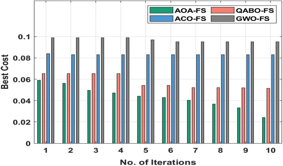
Figure 5: BC analysis of AOA-FS technique on Australian credit dataset
4.1 Comparative Results Analysis on AnalcatData Dataset
Tab. 2 offers a brief comparative study of the ODL-FCP with other techniques on the AnalcatData dataset.
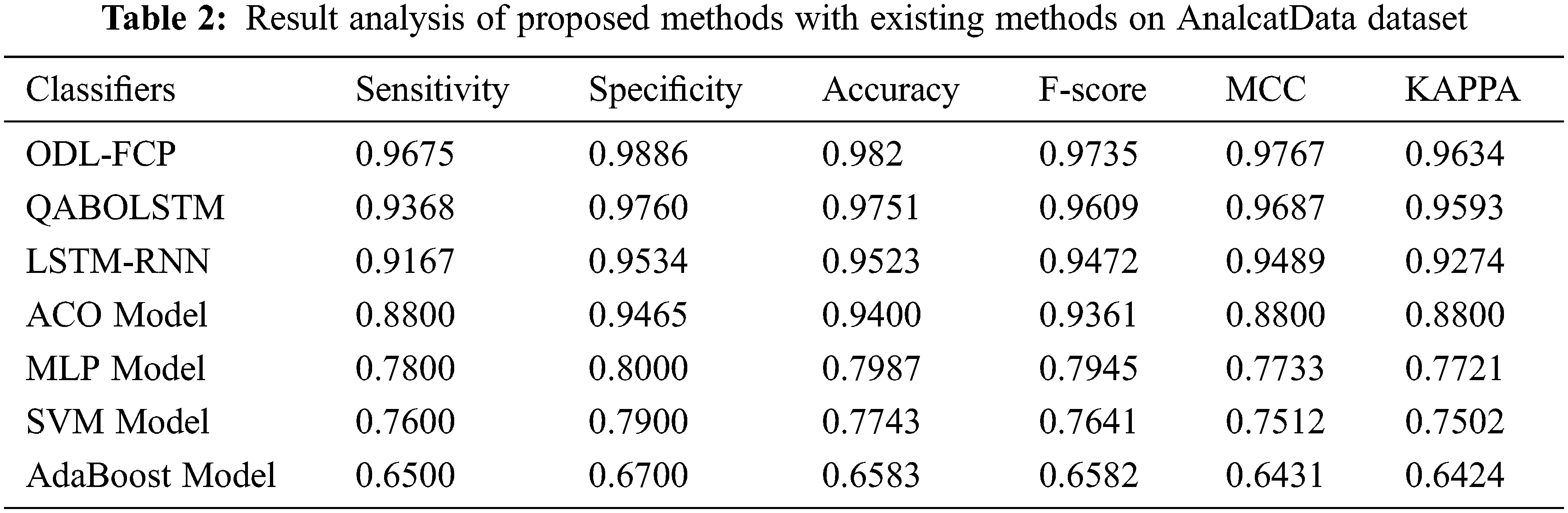
Fig. 6 offers the
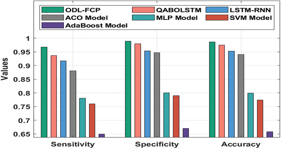
Figure 6:
Fig. 7 provides the
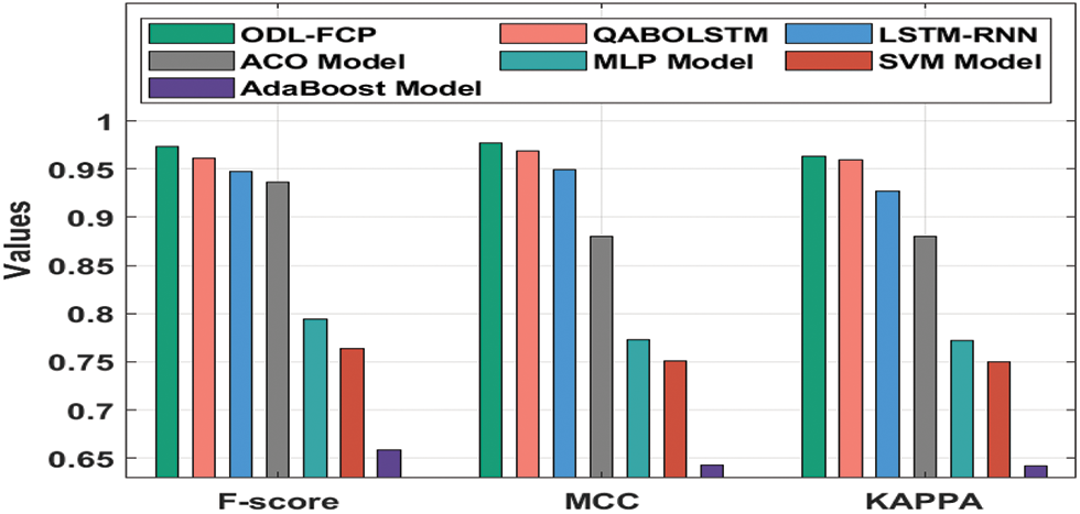
Figure 7:
4.2 Comparative Results Analysis on German Credit Dataset
Tab. 3 provides a brief comparative analysis of the ODL-FCP with other approaches on the German Credit dataset. Fig. 8 suggests the
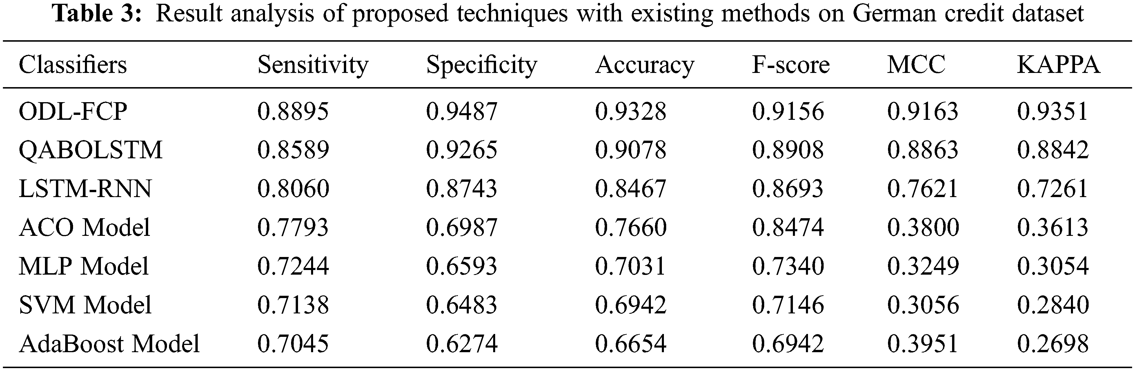
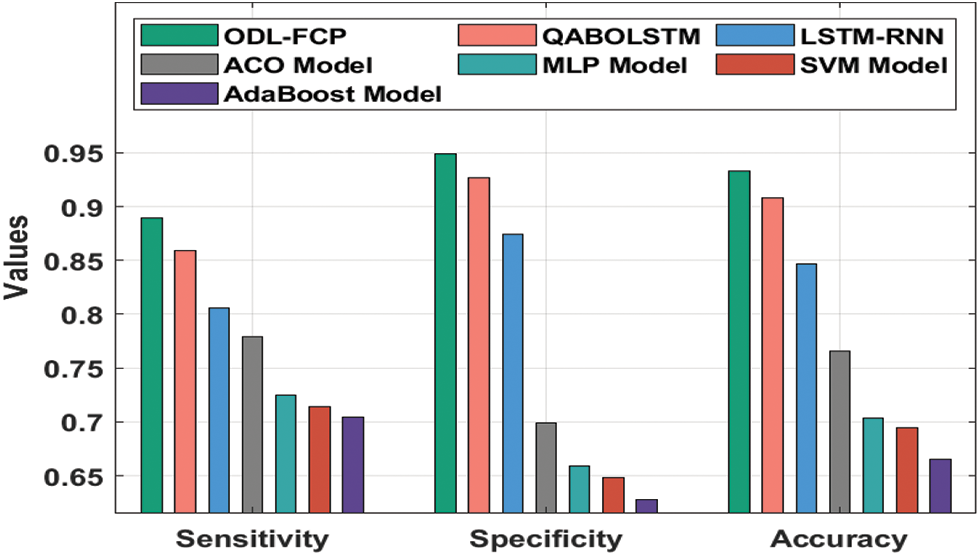
Figure 8:
Fig. 9 gives the
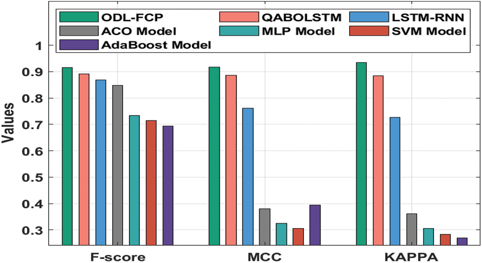
Figure 9:
4.3 Comparative Results Analysis on Australian Credit Dataset
Tab. 4 depicts a detailed comparative analysis of the ODL-FCP with other techniques on the Australian Credit t dataset. Fig. 10 shows the
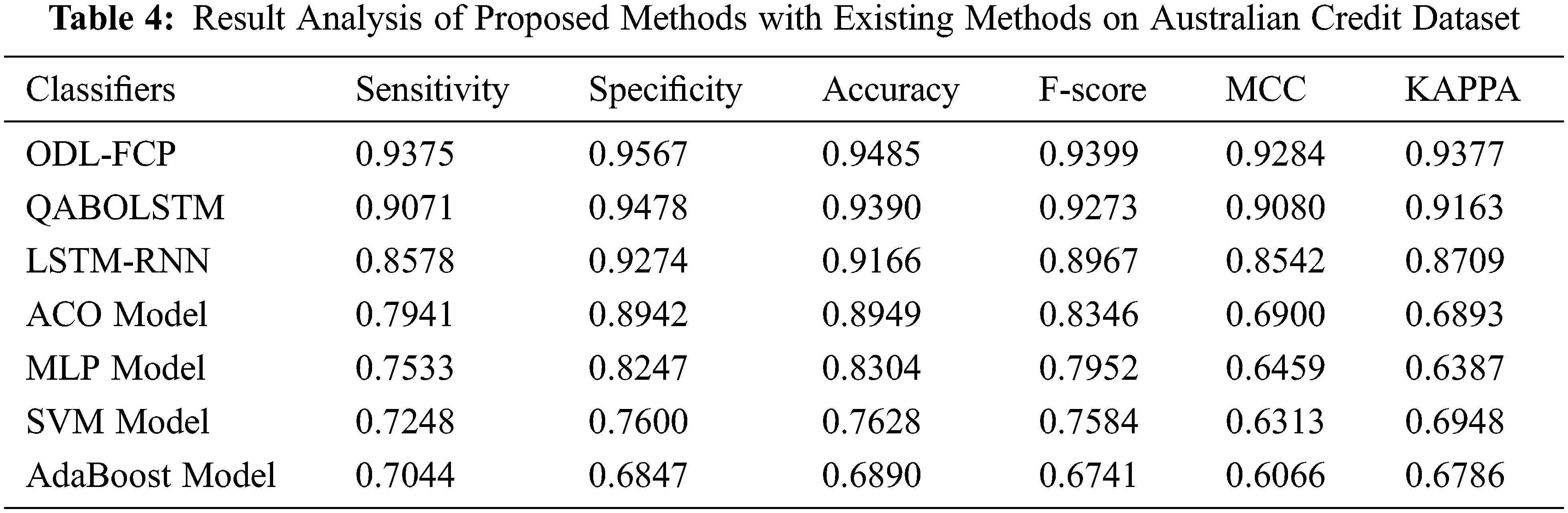
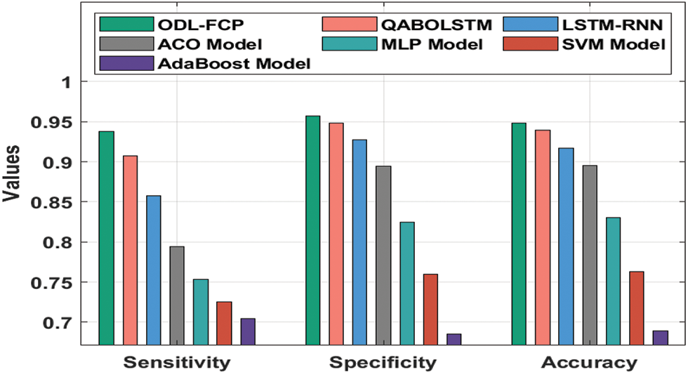
Figure 10:
Fig. 11 examines the
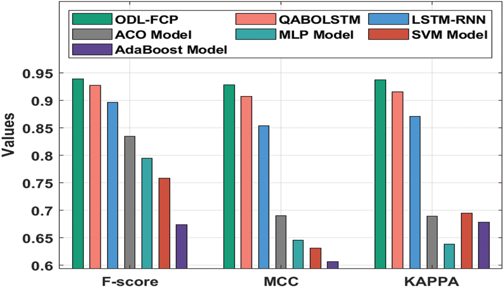
Figure 11:
From the detailed results and discussion, it can be ensured that the ODL-FCP technique can be applied as a proficient method to determine the financial crisis of SMEs.
In this paper, an efficient ODL-FCP technique has been presented for the identification of the financial crisis of SMEs. The proposed ODL-FCP technique encompasses major subprocesses namely pre-processing, AOA-based selection of features, CNN-LSTM based classification, and SFO based hyperparameter tuning. The utilization of AOA for the optimal selection of features and SFO for the hyperparameter optimization process aid to accomplish improved classification performance. To showcase the enhanced classification performance of the ODL-FCP technique, a wide range of simulations were carried out against benchmark financial datasets and the outcomes are examined concerning various metrics. The experimental results highlighted that the proposed ODL-FCO technique has outperformed the other techniques. As a part of future extension, the ODL-FCP technique is extended to the design of data clustering approaches in a big data environment.
Funding Statement: The authors received no specific funding for this study
Conflicts of Interest: The authors declare that they have no conflicts of interest to report regarding the present study.
1. M. Ala’raj and M. F. Abbod, “Classifier’s consensus system approach for credit scoring,” Knowledge-Based System, vol. 104, pp. 89–105, 2016. [Google Scholar]
2. A. Martin, V. Aswathy, S. Balaji, T. M. Lakshmi and V. P. Venkatesan, “An analysis on qualitative bankruptcy prediction using fuzzy ID3 and ant colony optimization algorithm,” in International Conference on Pattern Recognition, Informatics and Medical Engineering (PRIME-2012), Salem, India, pp. 416–421, 2012. [Google Scholar]
3. Guojun Gan, Chaoqun Ma and Jianhong Wu, “Data clustering: theory, algorithm and application,” ASA-SIAM Series on Statistics and Applied Mathematics, Philadelphia, vol. 1, pp. 3–17, 2007. [Google Scholar]
4. A. Ekbal and S. Saha, “Joint model for feature selection and parameter optimization coupled with classifier ensemble in chemical mention recognition,” Knowledge Based Systems, vol. 85, pp. 37–51, 2015. [Google Scholar]
5. A. F. Atiya, “Bankruptcy prediction for credit risk using neural networks: A survey and new results,” IEEE Transactions on Neural Network, vol. 12, no. 4, pp. 929–935, 2001. [Google Scholar]
6. G. Ou, “Research on early warning of financial risk of real estate enterprises based on factor analysis method,” Social Scientist, vol. 9, no. 56, pp. 56–63, 2018. [Google Scholar]
7. Y. Yang, “Research on information disclosure of listed companies and construction of financial risk early warning system,” Modern Business, vol. 1, pp. 151–152, 2018. [Google Scholar]
8. M. Chen, “Predicting corporate financial distress based on integration of decision tree classification and logistic regression,” Expert Systems with Applications, vol. 38, no. 9, pp. 11261–11272, 2011. [Google Scholar]
9. Y. Lee and H. Teng, “Predicting the financial crisis by mahalanobis – Taguchi system – Examples of Taiwan’s electronic sector,” Expert Systems with Applications, vol. 36, no. 4, pp. 7469–7478, 2009. [Google Scholar]
10. V. Ravi and C. Pramodh, “Threshold accepting trained principal component neural network and feature subset selection: Application to bankruptcy prediction in banks,” Applied Soft Computing, vol. 8, no. 4, pp. 1539–1548, 2008. [Google Scholar]
11. W. Y. Lin, Y. H. Hu and C. F. Tsai, “Machine learning in financial crisis prediction: A survey,” IEEE Transactions on Systems, Man, and Cybernetics, Part C, vol. 42, no. 4, pp. 421–436, 2012. [Google Scholar]
12. J. Uthayakumar, N. Metawa, K. Shankar and S. K. Lakshmanaprabu, “Financial crisis prediction model using ant colony optimization,” International Journal of Information Management, vol. 50, no. 5, pp. 538–556, 2020. [Google Scholar]
13. B. Yan and M. Aasma, “A novel deep learning framework: Prediction and analysis of financial time series using CEEMD and LSTM,” Expert Systems with Applications, vol. 159, no. 4, pp. 113609, 2020. [Google Scholar]
14. S. Yang, “A novel study on deep learning framework to predict and analyze the financial time series information,” Future Generation Computer Systems, vol. 125, no. 12, pp. 812–819, 2021. [Google Scholar]
15. G. Perboli and E. Arabnezhad, “A machine learning-based DSS for mid and long-term company crisis prediction,” Expert Systems with Applications, vol. 174, no. 4, pp. 114758, 2021. [Google Scholar]
16. A. Samitas, E. Kampouris and D. Kenourgios, “Machine learning as an early warning system to predict financial crisis,” International Review of Financial Analysis, vol. 71, no. 2, pp. 101507, 2020. [Google Scholar]
17. J. Uthayakumar, N. Metawa, K. Shankar and S. K. Lakshmanaprabu, “Intelligent hybrid model for financial crisis prediction using machine learning techniques,” Information Systems and e-Business Management, vol. 18, no. 4, pp. 617–645, 2020. [Google Scholar]
18. S. K. S. Tyagi and Q. Boyang, “An intelligent internet of things aided financial crisis prediction model in FinTech,” IEEE Internet of Things Journal, vol. 10, pp. 1, 2021. [Google Scholar]
19. F. A. Hashim, K. Hussain, E. H. Houssein, M. S. Mabrouk and W. Al-Atabany, “Archimedes optimization algorithm: A new metaheuristic algorithm for solving optimization problems,” Applied Intelligence, vol. 51, pp. 1–21, 2020. [Google Scholar]
20. Z. M. Ali, I. M. Diaaeldin, A. El-Rafei, H. M. Hasanien, S. H. A. Aleem et al., “A novel distributed generation planning algorithm via graphically-based network reconfiguration and soft open points placement using Archimedes optimization algorithm,” Ain Shams Engineering Journal, vol. 12, no. 2, pp. 1923–1941, 2021. [Google Scholar]
21. I. E. Livieris, E. Pintelas and P. Pintelas, “A CNN-LSTM model for gold price time-series forecasting,” Neural Computing and Applications, vol. 32, no. 23, pp. 17351–17360, 2020. [Google Scholar]
22. M. Li, Y. Li, Y. Chen and Y. Xu, “Batch recommendation of experts to questions in community-based question-answering with a sailfish optimizer,” Expert Systems with Applications, vol. 169, no. 9, pp. 114484, 2021. [Google Scholar]
23. L. Wensheng, W. Kuihua, F. Liang, L. Hao, W. Yanshuo et al., “A region-level integrated energy load forecasting method based on CNN-LSTM model with user energy label differentiation,” in 5th Int. Conf. on Power and Renewable Energy (ICPRE), Shanghai, China, pp. 154–159, 2020. [Google Scholar]
24. T. Zheng, “Scene recognition model in underground mines based on CNN-LSTM and spatial-temporal attention mechanism,” in Int. Sym. on Computer, Consumer and Control (IS3C), Taichung City, Taiwan, vol. 20, pp. 513–516, 2020. [Google Scholar]
25. S. J. Bu, H. J. Moon and S. B. Cho, “Adversarial signal augmentation for CNN-LSTM to classify impact noise in automobiles,” in IEEE Int. Conf. on Big Data and Smart Computing (BigComp), Jeju Island, Korea (Southvol.10, pp. 60–64, 2021. [Google Scholar]
26. Y. Wang, X. Wang and X. Chang, “Sentiment analysis of consumer-generated online reviews of physical bookstores using hybrid LSTM-CNN and LDA topic model,” in Int. Conf. on Culture-Oriented Science & Technology (ICCST), Beijing, China, vol.24, pp. 457–462, 2020. [Google Scholar]
 | This work is licensed under a Creative Commons Attribution 4.0 International License, which permits unrestricted use, distribution, and reproduction in any medium, provided the original work is properly cited. |