Intelligent Automation & Soft Computing DOI:10.32604/iasc.2023.025437
Article

Hybrid Convolutional Neural Network and Long Short-Term Memory Approach for Facial Expression Recognition

M. N. Kavitha1,* and A. RajivKannan2

1Department of Computer Science & Engineering, Kongu Engineering College, Perundurai, Erode, 638060, Tamil Nadu, India
2Department of Computer Science & Engineering, K.S.R. College of Engineering, Tiruchengode, 637215, Tamil Nadu, India
*Corresponding Author: M. N. Kavitha. Email: kavithafeb1@gmail.com
Received: 23 November 2021; Accepted: 27 February 2022

Abstract: Facial Expression Recognition (FER) has been an important field of research for several decades. Extraction of emotional characteristics is crucial to FERs, but is complex to process as they have significant intra-class variances. Facial characteristics have not been completely explored in static pictures. Previous studies used Convolution Neural Networks (CNNs) based on transfer learning and hyperparameter optimizations for static facial emotional recognitions. Particle Swarm Optimizations (PSOs) have also been used for tuning hyperparameters. However, these methods achieve about 92 percent in terms of accuracy. The existing algorithms have issues with FER accuracy and precision. Hence, the overall FER performance is degraded significantly. To address this issue, this work proposes a combination of CNNs and Long Short-Term Memories (LSTMs) called the HCNN-LSTMs (Hybrid CNNs and LSTMs) approach for FERs. The work is evaluated on the benchmark dataset, Facial Expression Recog Image Ver (FERC). Viola-Jones (VJ) algorithms recognize faces from preprocessed images followed by HCNN-LSTMs feature extractions and FER classifications. Further, the success rate of Deep Learning Techniques (DLTs) has increased with hyperparameter tunings like epochs, batch sizes, initial learning rates, regularization parameters, shuffling types, and momentum. This proposed work uses Improved Weight based Whale Optimization Algorithms (IWWOAs) to select near-optimal settings for these parameters using best fitness values. The experimental findings demonstrated that the proposed HCNN-LSTMs system outperforms the existing methods.

Keywords: Facial expression recognition; Gaussian filter; hyperparameter optimization; improved weight-based whale optimization algorithm; deep learning (DL)

1  Introduction

FER in humans has developed into a significant subject of study in these twenty years. Humans transmit their emotions and intentions through the face and face is the most powerful, natural, and instantaneous way of assessing emotions. Individuals use facial expressions and verbal tones to infer emotions like joy, sadness, and anger. Computer visions recognize facial expressions that reflect anger, contempt, fear, pleasure, sadness, and surprise. Many studies [1,2] have pointed out that verbal components account for 1/3rd of human communications, while nonverbal components account for the balance 2/3rd. Facial expressions are nonverbal components that carry emotional meaning and are primary to interpersonal communications [3,4]. As a result, it’s no surprise that research into facial expressions has attracted much attention in recent decades [5]. Automated and real-time FERs have significant influences in many areas, including healthcare, human-computer interaction, safe driving, virtual reality, picture retrievals, video-conferencing, human emotion analyses, cognitive sciences, personality developments, and so on [6]. However, effective identification of facial emotions from images/videos remains a complex task where the challenges are inaccurately extracting emotional features.

Detections, feature extractions, and facial expressions categorizations are the basic phases in automated FERs. Studies have used several feature extraction approaches, including Scale-Invariant Feature Transform (SIFT) [7], Histograms of Oriented Gradients (HOGs) [8], Local Binary Patterns (LBPs) [9], and Local Gabor Binary Patterns (LGBPs) [10] for facial emotion identifications. These approaches performed well on small training sets but were constrained in generalizations and could not be adapted to FERs. Many Machine Learning Techniques (MLTs) have been proposed for classifying facial expressions, including Neural Networks (NNs), Support Vector Machines (SVMs), Bayesian Networks (BNs), and rule-based classifiers but failed to achieve acceptable recognition rates.

Despite the use of DLTs in FERs difficulties persist as they need a substantial quantity of training data to avoid overfitting [11]. Moreover, available databases/datasets on FERs are insufficient to train NNs with a deep architecture. NNs have been used in object identification tests successfully. FERs are also affected by significant inter-subject variances based on humans’ characteristics like age, gender, ethnicity, and level of expressiveness. Confusions are also added by variations in postures, lightings, and occlusions in unconstrained facial expression settings. These variables are nonlinearly associated with FERs and emphasize the need for DLTs to address high intra-class variations while and learning expression-specific representations effectively.

The study in [12] used the Toronto Face Database (TFD) dataset for FERs using multitask CNNs. Their scheme resulted in a success rate of 85.13%. Khorrami et al. [13] used zero-bias CNNs for facial expression identifications and achieved 88.6% in terms of accuracy. Khorrami et al. [14] proposed fine-tuned CNNs for predicting facial expressions. Their tests on the TFD dataset resulted in a success rate of 88.9 percent. However, CNN’s training choices directly impact performance successes where improving hyper-parameter optimizations can lead to enhanced accuracy in DLTs. Following this introductory section, a thorough examination of prior proposed FERs is examined followed by this study’s proposed FER design approach. The fourth section displays simulation results followed by conclusions and future projects.

2  Literature Review

Zhang et al. [15] created a joint expression modeling system for FERs based on Generative Adversarial Networks (GANs). The work used the generator’s encoder-decoder structure to learn facial images’ identity representations. Then, the authors used expressions and posture codes where identity representations were decoupled from both expressions and pose variants. The automated production of facial images with various expressions in arbitrary positions for expanding FERs training sets has been focused on in the final stage. Quantitative and qualitative assessments on controlled and uncontrolled datasets showed that their proposed algorithm outperformed most other techniques.

Zeng et al. [16] proposed a novel framework for FERs that could accurately discriminate expressions as it contained accurate and comprehensive information about emotions. The study introduced high-dimensional features encompassing facial geometry and appearances for its FER. In addition, DSAEs (Deep Sparse Auto Encoders) detected facial emotions with high accuracy by learning discriminative features robustly from data. Their experimental results showed that their framework had high recognition accuracies (95.79%) on the extended Cohn–Kanade (CK+) database and outperformed the other three benchmarked methods by 3.17%, 4.09%, and 7.41%. Their proposed scheme used eight facial emotions, including neutral expressions, for better recognition accuracy, demonstrating the practicality and effectiveness of the approach.

FaceNet2ExpNet presented by Ding et al. [17], was a unique idea in network-based training for expression recognition from static pictures. The scheme used a novel distribution function to describe the expression network’s high-level neurons. The work used a two-stage training method wherein the pre-training step, expressions trained CNNs and regularized by face net. Moreover, in the refining stage, they appended fully-connected layers to the pre-trained CNNs layers and jointly trained the entire network. Their visual findings demonstrated that their model captured better high-level expression semantics. Their evaluations on FERs datasets:CK+; Oulu-CASIA; TFD, and SFEW, showed excellent results compared to other techniques.

Li et al. [18] proposed a new and efficient Deep Fusion-CNNs (DF-CNNs) in their study for multimodal 2D/3D FERs. Feature extraction/ feature fusion subnets and a softmax layer constituted their DF-CNNs. Each textured three-dimensional face scan was represented as six 2D facial attribute maps (one geometry, three normal, one curvature, and one texture). These maps were fed into the proposed DF-CNNs for learning features and fusion resulting in highly concentrated facial representation (32-dimensional). The study used two methods for predicting expressions: 1) learning linear SVMs on 32-dimensional fused deep features and 2) directly predicting using softmax on the six-dimensional expression probability vectors. Their DF-CNN’s integrated feature/fusion learning into a single training architecture. The study illustrated the efficacy of DF-CNNs with extensive tests on three 3D facial datasets and compared it with the performance of DFCNN handmade features, pre-trained deep features, fine-tuned deep features, and other techniques (i.e., BU-3DFE Subset I, BU-3DFE Subset II, and Bosphorus Subset). Their proposed DF-CNN’s consistently outperformed other methods. This was probably the first paper to introduce deep CNN to 3D FERs and deep learning-based feature level fusion for multimodal 2D/3D FERs.

Sun et al. [19] proposed robust vectorized CNNs with an attention mechanism for extracting characteristics from facial ROIs (Region of Interests). This study designated facial ROIs before sending them to CNNs. The attention notion, in particular, was used as the first layer of their proposed NNs to conduct ROI-related convolution computations and extracted robust features. The study’s ROIs-related convolution outcomes on particular ROIs were found to be improved. The scheme used CapsNetin NNs next layer for the generation of feature vectors. Multi-level convolutions extracted feature vectors from distinct ROIs for facial expressions, which were subsequently rebuilt by a decoder to reconstruct the entire image. Their experimental findings showed that their suggested method was extremely successful in enhancing the performances of FERs.

Alenazy et al. [20] focused on predicting facial expressions in their study where the datasets CK+, Oulu CASIA, MMI, and JAFFE were used for testing. Their scheme was semi-supervised DBNs (Deep Belief Networks). For accuracy in FERs, the study used GSAs (Gravitational Search Algorithm) which improved specific parameters of DBMNs. The study for extracting features from lips, cheeks, brows, eyes, and furrows, their scheme used HOGs (Histogram Oriented Gradients) and 2D-DWTs (2D-Discrete Wavelet Transform). Their feature selections eliminated undesirable information from images. Their Kernel-based PCAs (Principal Component Analysis) extracted features. Their proposal also discovered non-linear components by obtaining higher-order correlations between input variables. Features derived from the lip patches using HOGs resulted in accurate facial emotion categorizations. Their results showed that any classifier based on DBN-GSA could produce accurate results.

Ryu et al. [21] introduce a novel face descriptor for FERs. Their facial emotion detections were called Local Directional Ternary Patterns (LDTPs) which effectively encoded emotion-related characteristic information including eyes, brows, upper nose, and mouth) with the help of directional information and ternary patterns, thus capitalizing on edge patterns’ strength in edge areas. They proposed histogram-based facial description methods which partitioned a human face into multiple areas and sampling codes. They used face descriptors with two-level grids while sampling expression-related information using different scales. One was a coarse grid for stable codes (closely connected to non-expressions) and a finer grid for active codes (highly related to expressions). Their multi-level technique allowed the description of facial movements at a finer granularity while maintaining coarse expression characteristics. The study learned from LDTPs codes from emotion-related facial areas where their experimental results suggested that their designed technique enhanced overall FERs accuracy values.

3  Proposed Methodology

This study proposes the HCNN-LSTMs approach for FERs where the proposed scheme is divided into four stages: pre-processing, facial detections, feature extractions, and classifications. Fig. 1 depicts the workflow of the proposed scheme.

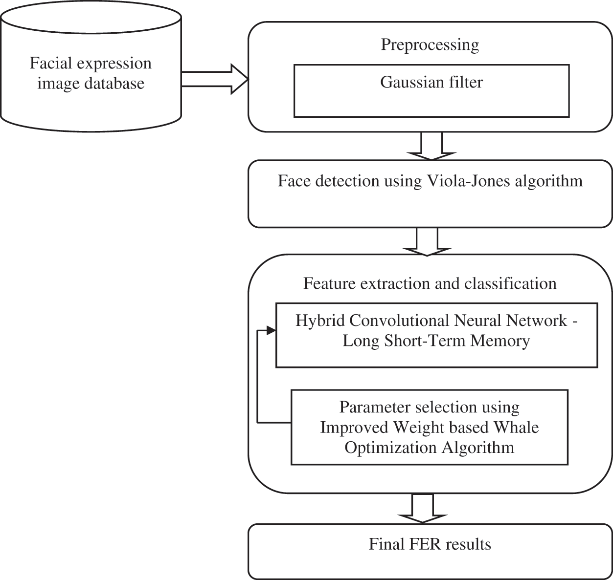
Figure 1: Flow diagram of the proposed work

3.1 Input

In this work, FERC Dataset is taken as the input for facial expression recognition. It contains two directories, namely train and test and file labels. Both train and test directories contain seven classes: anger, disgust, fear, happiness, neutral, sadness, and surprise.

3.2 Preprocessing Using Gaussian Filter

Pre-processing facial pictures is a very crucial process in FER. The image noises can be filtered using filters, and this study uses GFs (Gaussian Filters) to smoothen noises present in facial images. The GFs usage based on a 2-D convolution smoothing operator where current image pixel values are replaced by weighted mean computed from the pixel’s neighborhood. This weight decreases as the pixel’s distance from the centre increases. GFs are similar to mean filters but use a different kernel to reflect Gaussian (‘bell-shaped’) humps. Eq. (1) represents 2D Gaussian distributions with 0 and standard deviation σ = 1.

G(x,y)=12πσ2e−x2+y22σ2 (1)

where, σ is the standard deviation and x, y is the local coordinate of an image.

3.3 Facial Detections Using VJ Algorithm

The faces from images are detected using VJ algorithm in this research work. This technique is used as it has high detection rates in real-time data. This VJ algorithm can be divided into four stages: Haar feature selections, integral images, Adaboost training, and cascading classifiers.

3.3.1 Haar Feature Selections

Haar features are visual characteristics used for object detection. VJ algorithm modifies Haar wavelet concepts to generate Haarlike characteristics. Many humans share a few common characteristics, like eyes in images are darker than their neighboring pixels while the nose region looks brighter than the eyes. Haar features can be assessed where two or three rectangles are used to determine the existence of a face in images. Each Haar feature’s value can be computed by calculating the area of each rectangle and then adding it up. Fig. 2 shows the haar features.

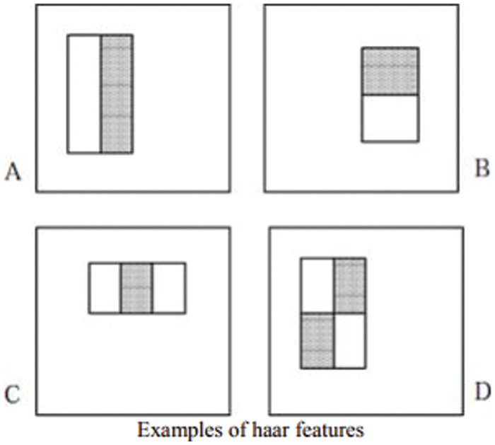
Figure 2: Haar features

3.3.2 Creating an Integral Image

Integral images are a kind of image representation used in the pre-processing phase, and integral images are computed. VJ algorithm starts by converting input facial images into integral images, which is accomplished by setting each pixel equal to the total sum of all pixels above and to the left of the pixel. Integral images can be computed using Eq. (2):

I(x,y)=∑x′≤x,y′≤y⁡o(x,,y,) (2)

where I - integral image and O - original image

Integral images are summations of rectangular regions where the sum of all pixels within a rectangular region Z = [A1, A2, A3, A4] can be computed using Eq. (3)

I(x,y)=∑(x,y)∈z⁡O(A4)+O(A1)+O(A2)+O(A3) (3)

Features are determined in a specified time since the sum of the pixels in the component rectangles can be computed in constant time. VJ discovers the values through a detector and a basic resolution of 24*24 pixels for producing good results.

3.3.3 AdaBoost Based Raining

AdaBoost is an MLT that finds the correct hypothesis by combining multiple weak hypotheses with average accuracy. Adaboost is used in this work as it aids in the selection of only the best features in a pool of features. Once it establishes required features, a weighing of features is used to determine if the feature is the part of the window with a face. The characteristics are often called weak classes.

3.3.4 Cascading Classifiers

The use of multiple/cascade of sophisticated classifiers can produce higher detection rates. VJ face detection algorithm works by scanning detectors often with different sizes of the same image where the disproportionate number of assessed sub-windows may not face. Cascade classifiers are made of layers where each layer has a powerful classifier, and each level is responsible for determining if a particular sub-window is a face/non-face.

3.4 Feature Extractions and Classification

This research work uses HCNN-LSTMs for its feature extractions and facial expression categorizations. The CNNs used in the study include training alternatives that can directly impact performance successes. The essential parameters for training include maxepochs, minbatch sizes, initial learning rates, regularization parameters, shuffle types, and momentum. This work’s IWWOAs select near-optimal settings of parameters used in this work.

3.4.1 CNNs

CNN is one of the most powerful DLTs that can function with several hidden layers, convolute these layers, and sub-sample to extract low/high-level features from input data. CNN typically has convolution, sub-sampling/pooling, and fully connected layers as depicted in Fig. 3.

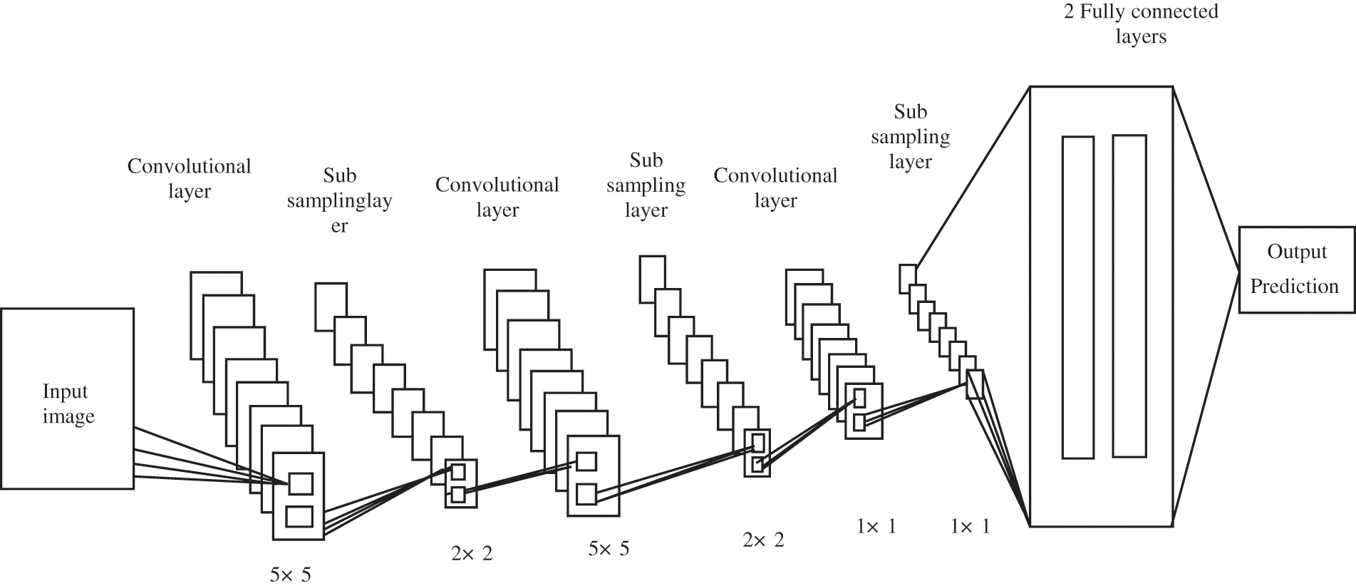
Figure 3: CNNs

This work uses CNNs for two main things: feature extractions and classifications. Multiple convolution layers are used for feature extractions, and max-pooling and activation functions are subsequently used. Classifiers are typically made up of completely linked layers.

3.4.2 Convolution Layer

Convolution layer is a key component of CNNs in this study and is used for feature extractions. It includes linear/non-linear processes including convolution and activation functions. Input features are convolved with a kernel in this layer for filtering (convolution matrix kernels) and producing n output features identified from input images. The output features are generated by convolving the kernel and inputs referred to as feature maps of size i*i.

CNN has many convolution layers, and output features are inputs to subsequent convolution layers. Each convolution layer has n filters convolved with inputs, resulting in (n*) feature maps, which equals the number of filters used in convolutions. It should be noted that each filter map is regarded as a distinct feature at a given position in inputs. The outputs from lth convolution layer denoted by Ci(l) , has feature maps and computed using Eq. (4)

Ci(l)=Bi(l)+∑j=1ai(l−1)⁡Ki,j(l−1)∗Cj(l) (4)

where, Bi(l) is the bias matrix and Ki,j(l−1) is convolution filter or kernel of size a*a that connects the j-th feature map in layer (l − 1) with the i-th feature map in the same layer. The output Ci(l) layer consists of feature maps. In Eq. (5), the first convolutional layer Ci(l−1) is input space, that is, Ci(0)=Xi . The kernel generates feature map. After the convolution layer, the activation function can be applied for nonlinear transformation of the outputs of the convolutional layer

Yi(l)=Y(Ci(l)) (5)

where, Yi(l) - output of the activation function, Ci(l) - input that it receives. CNNs generically use activation functions which may be sigmoid, tanh, and ReLUs (rectified linear units). This research work uses ReLUs depicted in Eq. (6)

Yi(l)=max(0,Yi(l)) (6)

ReLUs are used in DLTs as it reduces interactions and nonlinear effects. When the input is negative, ReLUs convert outputs to 0 while positive values are unchanged. The main advantage of activation functions is its accommodation of quicker training based on an error derivative, which becomes extremely tiny in the saturating area, and therefore weights that get updated virtually disappear also referred to as vanishing gradient problem.

3.4.3 Sub-Sampling/Pooling Layer

Reducing dimensionality of input features maps produced from preceding convolutions is the primary goal of this layer. Sub-sampling process is carried out between masks and feature maps where a mask of size bb is chosen. The sub-sampling procedure between masks and feature maps can be depicted mathematically as Eq. (7).

Xjl=f(βjldown(Xjl−1)+bjl) (7)

where down (•) is a sub-sampling function and sums each individual n-by-n features in the input t, resulting in an output that is n-times smaller in spatial dimensions. Each output map has its own multiplicative bias and additive bias b.

3.4.4 Fully Connected Layer

The convolution layers extracted features and were sampled by pooling layers translated into the network’s final output. The probabilities for each class in classification tasks are a subset of fully connected layers. The Softmax activation function used in the output layer and detailed below:

Yi(l)=f(zi(l)) (8)

zi(l)=∑i=1mi(l−1)⁡wi,j(l)yi(l−1) (9)

where, wi,j(l) are the weights adjusted in the fully connected layer for constructing representations of each class, and f is a transfer function that represents non-linearity. The fully linked layer’s non-linearity is constructed through neurons, instead of distinct layers like convolution/pooling layers.

3.4.5 LSTMs

The LSTMs are a type of RNNs (Recurrent Neural Networks), but describe temporal sequences and long-term relationships within them better than standard RNNs. Fig. 4 depicts a typical LSTM cell that encompasses input, forget and output gates along with a cell activation component. These devices receive activation signals from multiple sources and use specific multipliers to regulate cell activations.

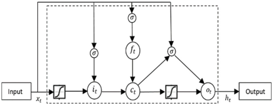
Figure 4: Long short term memory cell

The input gate of LSTM is defined as

it=σ(Wxixt+Whiht−1+Wcict−1+bi) (10)

The forget gate is defined as

ft=σ(Wxfxt+Whfht−1+Wcfct−1+bf) (11)

The cell gate is defined as

ct=ftct−1+ictanh(Wxcxt+Whcht−1+bc) (12)

The output gate is defined as

ot=σ(Wx0xt+Wh0ht−1+Wc0ct+b0) (13)

Finally, the hidden state is computed as

ht=ottanh(ct) (14)

tanh - hyperbolic tangent activation function, xt - input at time t and W and b - network parameters (Weights and Biases).

The σ is the logistic sigmoid function, and i, f, o and c are respectively the input gate, forget gate, output gate and cell state. Wci, Wcf and Wco are denoted weight matrices for peephole connections. In LSTM, three gates (i, f, o) control the information flow. Input gates determine input ratios which influence determining cell states (12). Forget gates determine whether prior memory ht1 is passed where prior memory ratio is derived based on Eq. (10) and used in the Eq. (12). Output gates decide if a memory cell’s output is passed and depicted as Eq. (14). LSTMs address the vanishing gradient issue with the use of these three gates. LSTM cells replace the recurrent hidden layer in the LSTM-RNN architecture.

The proposed HCNN-LSTMs approach takes a facial image as input and extracts features followed by dimensionality reduction where two layers of CNNs are used. The convolution layers use learnable filters to identify certain characteristics in the original image where different filters identify them and convolve them, resulting in a set of activation maps. These generated maps are then fed into LSTMs after being reduced in spatial dimensionality. LSTMs further acquire temporal features of images for accurate recognition of facial expressions. The two fully connected layers that existed in CNN architecture which refers to FC1 and FC2 are used to categorize the facial emotion recognition as happiness, disgust, fear, angry, neutral, sad and surprise based on the probabilities for each class in classification tasks. Fig. 5 shows the architecture of the proposed HCNN-LSTM.

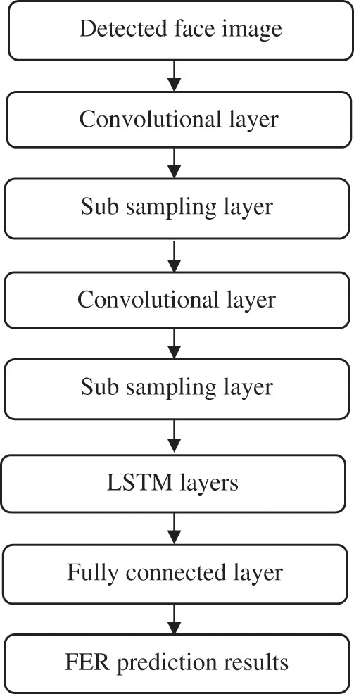
Figure 5: Hybrid CNN-LSTM model

3.4.6 Parameter Selection Using IWWOAs

Increasing the number of training samples directly affects the success rates of DLTs. Tuning DLT’s hyperparameters like max epochs, min batch sizes, initial learning rates, regularization parameters, shuffle types, and momentum improves the model’s performances. This work’s proposed IWWOAs select near-optimal settings for these parameters based on which CNNs train on adjusted hyperparameter values. Finally, the testing set is categorized using a trained model to assess the effectiveness of the suggested technique.

Mirjalili and Lewis presented a meta-heuristic nature-inspired that mimics the real-life behavior of whales. WOAs are swarm-based, mimicking humpback whales’ social behavior and inspired by their bubble-net tactics while hunting. These whales are the biggest group of baleen whales and always stand together. They hunt tiny groups of krill and small fish near the surface by forming bubbles along with a spiral pattern around their prey and then swimming up to the surface along this path. Their behaviors can be represented numerically.

Encircling of Prey: Maxepochs, small batch sizes, initial learning rate, regularization parameters, shuffle types, and momentum are treated as the whale population Xi( i = 1, 2, 3, …, n). Recognitions are imagined as a fitness function. Humpback whales can detect the presence of prey and encircle it where WOAs assume that the current best candidate solution is either the targeted optimal value or a value near to the target optimal value. When the best search agent is determined, other search agents attempt to update their locations about the best search agent and depicted by the following equations:

D→=|C→.X∗→(t)−X→(t)|, (15)

X→(t+1)=X∗→(t)−A→.D→, (16)

To improve the performance of the WOAs, this work uses a time-varying inertia weight along with the update Eq. (16). Inertia weight ω is defined in Eq. (17).

ω=(ω1−ω2)(Itermax−IterIter)+ω2 (17)

X→(t+1)=ω.X∗→(t)−A→.D→ (18)

where, ω1 is initial value of the inertia weight, ω2 final values of the inertia weight, iter current iteration, the Itermax is the maximum number of allowable iteration, it represents the present iteration A→ and C→ refer to the coefficient vectors. The X∗ indicates the location vector of the best solution, which is acquired till now and X∗→ stands for the location vector. X has to be updated through iteration if a better solution exists.

The vectors A→ and C→ are computed as below:

A→=2a→.r→−a→ (19)

C→=2.r→ (20)

where ′a′→ is linearly reduced from two to zero with the number of iterations. ‘r’ represents the random vector in the range [0,1].

As discussed in the preceding section, humpback whales use the bubble-net technique to attack their prey. The following is a mathematical formulation of this approach.

Exploitation Phase: This phase is called a bubble net attack, where operations are based on two mechanisms as detailed below:

Shrinking Encircling Technique: Locating the search agent randomly A→ in the interval [–1, 1] and between the agent’s earlier and current best positions.

Spiral Updating Position: The distance between the whale and prey located at (X, Y) and (X∗,Y∗) is computed, and a spiral equation between the position of whale and prey is created based on the following Eq. (21):

X→(t+1)=D′.→ebl.coscos(2πl)+ω.X∗→(t) (21)

Exploration Phase: WOAs achieve global optimizations. In Fig. 3, whales seek prey based on random locations or allow search agents to navigate from a reference whale, A→ is set in the interval, [–1,1]. Moreover, the positions of search agents are updated by randomly selecting agents making WOAs execute global searches. The following equations mathematically depict these exploration scans:

X→(t+1)=Xrand→−A→.D→ (22)

where, Xrand→ - random position of a whale selected randomly from the population.

The main steps of the proposed HCNN-LSTMs are described as follows

1: Prepare the Dataset

2: Process Face alignments

3: Convert RGB images to grayscale

4: Apply GDs for reducing noises

5: Facial detections

6: Split data into Training and Testing sets

7: Apply HCNN-LSTMs

8: Set initial values for IWSO control parameters

9: Set initial values for SwarmSize

10. Set initial values for of MaxIter

11: Set initial values for the fitness function

12: Execute until stop criterion of IWSO is not achieved

13: Perform IWSO algorithmic phases

14: Obtain near-optimal values for the hyperparameter as output

15: Train HCNN-LSTMs on the Training Set and tune hyperparameters

16: Output the trained model

17: Evaluate the success of HCNN-LSTMs on the Testing Set by using the trained model

4  Experimental Results

Python was used in implementations of the proposed HCNN- LSTMs FERs and tested on FERC dataset found on https://www.kaggle.com/manishshah120/facial-expression-recog-image-ver-of-fercdataset. The dataset had train and test folders with a labels file. In train/test image directories, seven expressive faces: anger, disgust, fear, happiness, neutral, sorrow, and surprise were found in train/test images directories. HCNN- LSTMs performances were compared with LSTMs and CNNs in terms of accuracy, precision, recall, and f-measures for FERs where the proposed scheme outperformed compared techniques, and their results are displayed in this section.

Initially, the input is taken from the FERC of Dataset and filtered using a Gaussian filter. The input and filtered image is represented in Figs. 6 and 7 respectively.

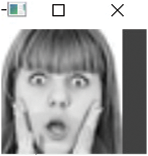
Figure 6: Input image

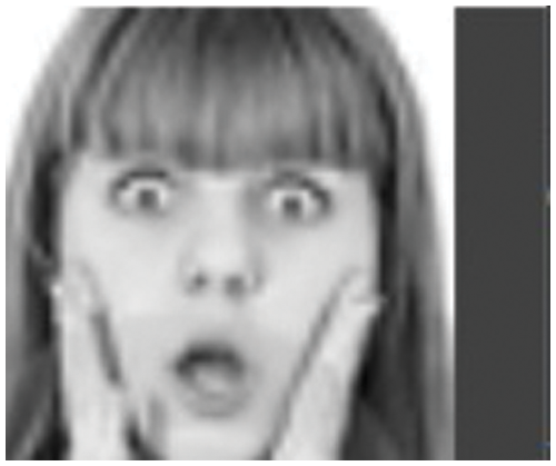
Figure 7: Filtered image

4.1 Accuracy

The measurement accuracy correctly identifies the weighted percentage of facial expressions. It is represented as,

Accuracy=TP+TNTP+FP+TN+FN (23)

where,

TP-True Positive

TN-True negative

FP-False Positive

FN-False Negative

4.2 Precision

Precision is the ratio of properly predicted positive results to the total predicted observations.

Precision=TPTP+FP (24)

4.3 Recall

Recall is the ratio of correctly predicted positive results to all observations in actual class.

Recall=TPTP+FN (25)

4.4 F-Measure

F-measure has represented the weighted average of precision and recall.

F=2P×RP+R (26)

Tab. 1 lists the comparative performance of the proposed HCNN-LSTMs on FERs with existing LSTMs and CNNs.

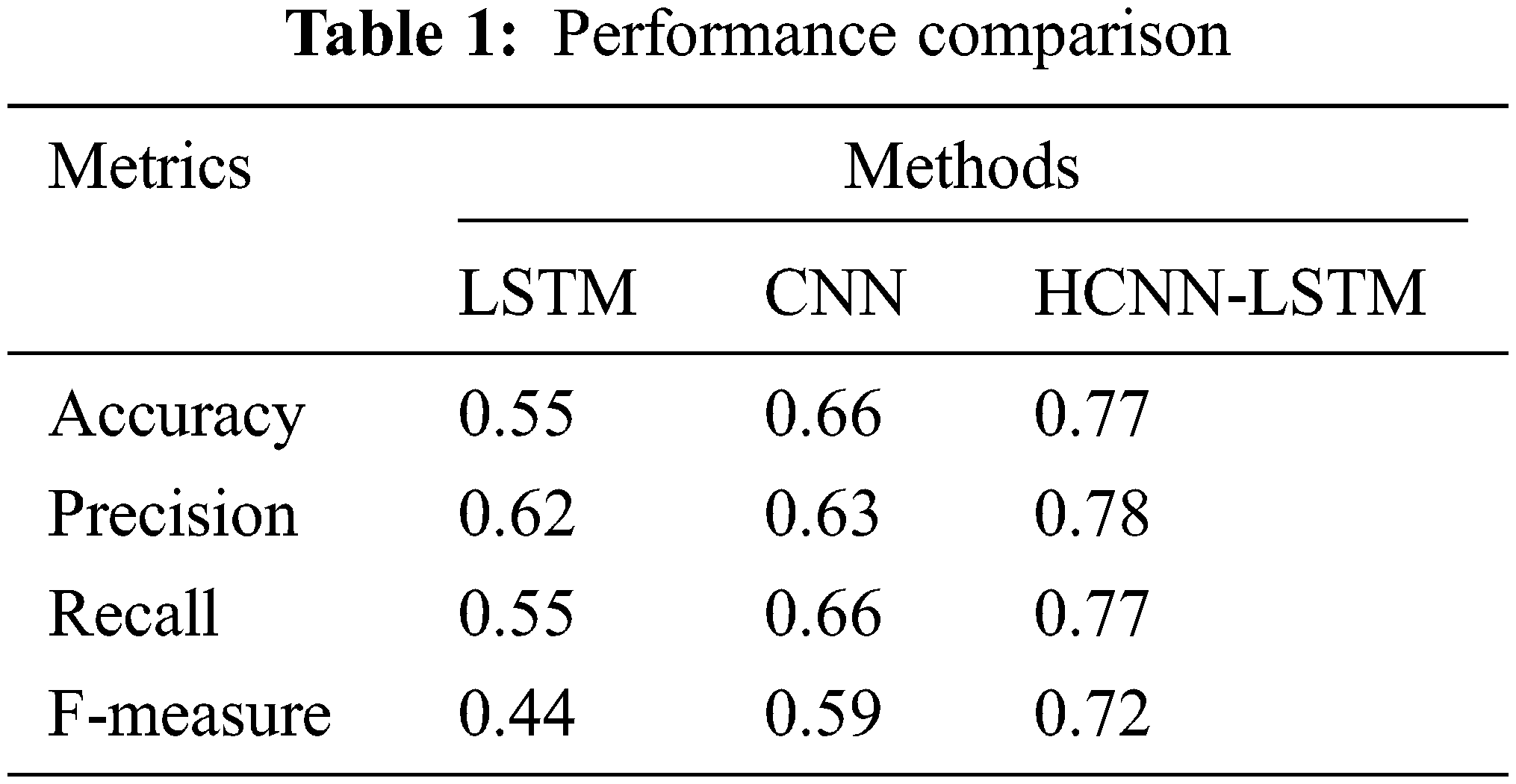
Fig. 8 shows iterations of the fitness function based on the data with recognition errors as output. It can be inferred that values decrease when iteration counts increase.

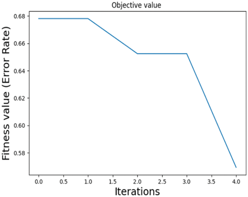
Figure 8: Fitness value

Fig. 9 shows the performance comparison. The proposed HCNN-LSTMs were compared with existing LSTMs and CNNs for FERs. The proposed system showed better performance in increased precision as it tuned hyperparameters using IWWOAs. This work’s experimental results showed that the suggested HCNN-LSTMs achieved 0.77% accuracy compared to LSTMs and CNNs accuracy values of 0.55% and 0.66% respectively. In terms of precision values the proposed system achieved a value of 0.78 when compared to 0.62 (LSTMs) and 0.63 (CNNs). According to the graph, the recall scores of HCNN-LSTMs suggested the proposed system had a recall of values of 0.77, whereas LSTMs and CNN scored 0.55 and 0.66, respectively. The suggested system’s f-measure value was 0.72, while LSTMs and CNNs f-measure values were 0.44 and 0.59, respectively.

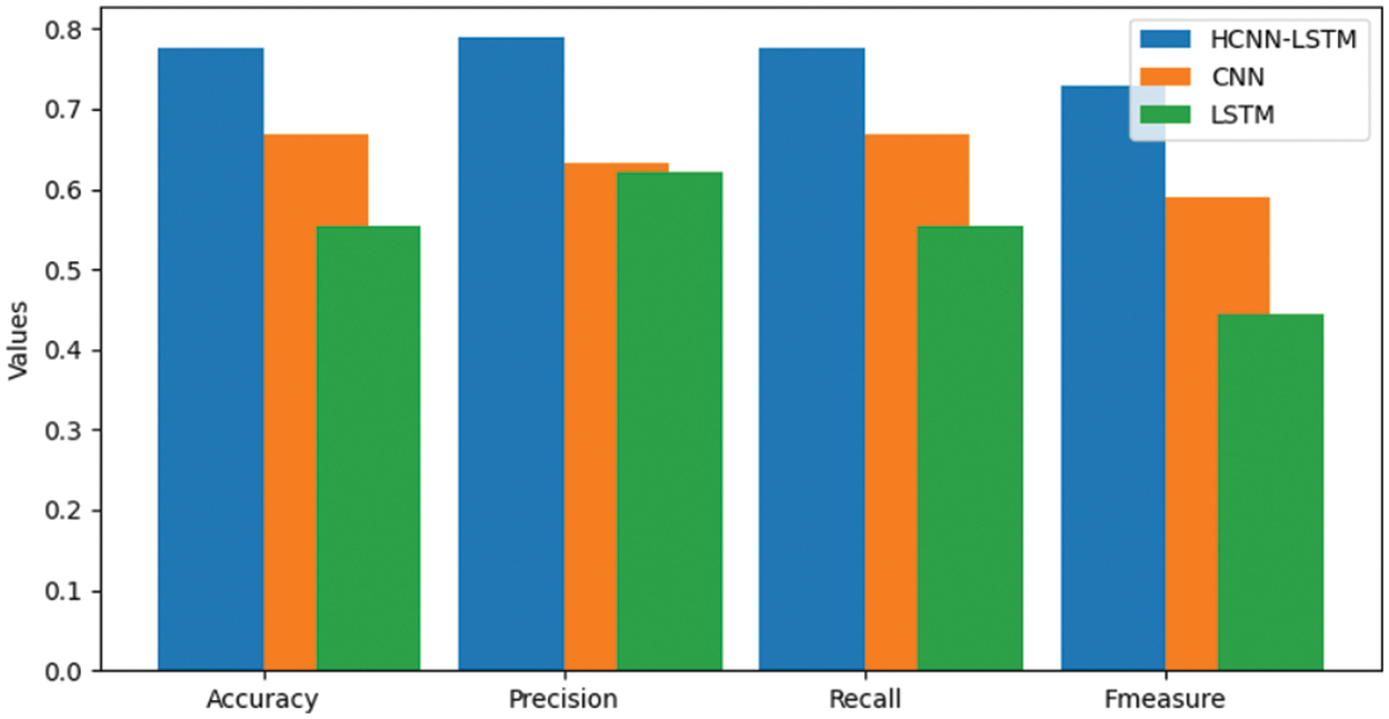
Figure 9: Performance comparison

5  Conclusion

This research work has proposed and demonstrated an approach for FERs called HCNN-LSTMs, a Hybrid approach combining CNNs with LSTMs. GFs eliminate noise from images in this work, and VJ algorithm identifies faces. This study increased the recognition rates by its use of the proposed HCNN-LSTMs in feature extractions and classifications. CNN use the parameters of maxepochs, min batch sizes, initial learning rates, regularization parameters, shuffle types, and momentum in training which IWWOAs tuned to select near-optimal hyperparameter values. This study’s experimental findings demonstrated the proposed system’s superior performances by outperforming prior systems in accuracy, precision, recall, and f-measure.

Funding Statement: The authors received no specific funding for this study.

Conflicts of Interest: The authors declare that they have no conflicts of interest to report regarding the present study.

This work is licensed under a Creative Commons Attribution 4.0 International License, which permits unrestricted use, distribution, and reproduction in any medium, provided the original work is properly cited.