DOI:10.32604/iasc.2022.029660
| Intelligent Automation & Soft Computing DOI:10.32604/iasc.2022.029660 | |
| Article |
Application of CNN and Long Short-Term Memory Network in Water Quality Predicting
1College of Engineering and Design, Hunan Normal University, Changsha, 410081, China
2Hunan Institute of Metrology and Test, Changsha, 410014, China
3Big Data Institute, Hunan University of Finance and Economics, Changsha, 410205, China
4University Malaysia Sabah, Sabah, 88400, Malaysia
*Corresponding Author: Jianjun Zhang. Email: 87890878@qq.com
Received: 09 March 2022; Accepted: 19 April 2022
Abstract: Water resources are an indispensable precious resource for human survival and development. Water quality prediction plays a vital role in protecting and enhancing water resources. Changes in water quality are influenced by many factors, both long-term and short-term. Therefore, according to water quality changes’ periodic and nonlinear characteristics, this paper considered dissolved oxygen as the research object and constructed a neural network model combining convolutional neural network (CNN) and long short-term memory network (LSTM) to predict dissolved oxygen index in water quality. Firstly, we preprocessed the water quality data set obtained from the water quality monitoring platform. Secondly, we used a CNN network to extract local features from the preprocessed water quality data and transferred time series with better expressive power than the original water quality information to the LSTM layer for prediction. We choose optimal parameters by setting the number of neurons in the LSTM network and the size and number of convolution kernels in the CNN network. Finally, LSTM and the proposed model were used to evaluate the water quality data. Experiments showed that the proposed model is more accurate than the conventional LSTM in the prediction effect of peak fitting. Compared with the conventional LSTM model, its root mean square error, Pearson correlation coefficient, mean absolute error and mean square error were respectively optimized by 5.99%, 2.80%, 2.24%, and 11.63%.
Keywords: LSTM; CNN; dissolved oxygen; water quality predicting
The importance of water to human life is self-evident, human survival and development are closely associated with water resources. With the rapid development of China’s social economy, many industrial wastes and pollutants have also been discharged into nature [1], far beyond nature’s self-purification capacity. At present, most of the rivers in China have been polluted to varying degrees, and some lakes are also in a state of eutrophication. Among the 112 key lakes in the country, the fifth type of water is close to 10% [2,3]. A significant increase in water pollution load has led to a significant increase in plankton and plants in water [4], and water hypoxia has become a serious worldwide problem. Dissolved oxygen is the amount of free oxygen in the water. Hypoxia in water will have many adverse effects. Hypoxia death of aquatic organisms such as fish and harmful gases released from sediments will damage the water [4]. Therefore, the content of dissolved oxygen in water is an important indicator to measure the self-purification capacity of the water body. When the dissolved oxygen in the water decreases, the time it takes to return to the initial state is shorter, indicating that the self-purification ability of the water body is stronger [5]. Improving the accuracy of dissolved oxygen prediction is not only beneficial to enhancing water quality, but also beneficial to river management and early warning. However, dissolved oxygen has the characteristics of time series, instability and non-linearity. The complex coupling relationship between various factors and the influence of various factors will affect the prediction results. Therefore, it is significant to select a suitable model to predict dissolved oxygen data.
With the continuous development of Internet of Things technology and the Internet, the digital economy is developing rapidly, and big data and related technologies are increasingly altering our daily life. By analyzing the big data generated in production and life [6,7], we can forecast the future [8,9]. According to the definition of time series characteristics [10], water quality indicators conform to time series characteristics, and the time series prediction model is suitable for water quality data prediction. In earlier studies. Scholars proposed a series of statistical prediction models such as the autoregressive integrated moving average (ARIMA) model based on time series analysis and variant seasonal autoregressive integrated moving average (SARIMA) model [11]. The unified feature of these models is that they need to test the steadiness and white noise of data. Due to lack of the ability to extract features from nonlinear data, traditional machine learning algorithms have more or less limitations in accuracy, convergence speed, and applicability [12].
In recent years, with the rapid development of neural networks and deep learning algorithms, they have been widely used in all walks of life [13]. Reshma et al. used a deep learning algorithm to estimate skin lesions by analyzing images [14]. Liu et al. proposed an attention-based cyclic neural network model, which can be used for human wearable activity recognition [15]. Xiang et al. proposed a spam detection model based on LSTM, which can effectively extract the time features of different product entities and perform fusion analysis on these features, effectively enhancing spam detection accuracy [16]. Wei et al. proposed a prediction model based on the LSTM network, trained wind speed data collected by WindLog wind speed sensor, and predicted wind speed 1, 5, and 10 minutes in advance [17]. Yan et al. proposed a short-term traffic flow prediction method based on the CNN-LSTM model. This network structure combined the ability of the CNN model to mine the spatial correlation of traffic flow with the ability of the LSTM model to mine the temporal characteristics of traffic flow, which could better realize short-term traffic flow prediction [18]. Lu et al. proposed a CNN-LSTM hybrid neural network model for short-term power load prediction. Firstly, CNN was applied to extract feature vectors at the bottom of the network. Then the extracted feature vectors are constructed according to the time series. Finally, the newly constructed time series is used as the input of LSTM for prediction [19]. Wang et al. used the advantages of CNN in capturing local correlation of data and LSTM in capturing data sequence and long-range dependence for typical commands and disguised intrusion commands so as to distinguish better and detect whether users’ behaviors are disguised intrusion behaviors [20]. Kumar et al. used recursive neural network and LSTM (RNN-LSTM) network to control different gates to control information input and state update methods, enabling them to mine long-distance sequential data information to forecast the stock market [21].
Among the various deep learning frameworks, CNN requires fewer parameters and is well suited for processing data with statistical stationarity and local correlation. LSTM neural networks are specially designed to learn time series data with long-term dependencies and have great advantages in learning long-term dependencies and temporality in higher-level feature sequences. These characteristics are very suitable for the needs of water quality prediction [21]. The main contributions of this paper can be summarized as follows: (1) a hybrid model for water quality prediction is proposed, which combines the respective advantages of the CNN model and LSTM. After the feature extraction of the CNN layer, the original data will get a new sequence with more vital feature ability than the original sequence. Then, the new sequence is put into the LSTM model, which is more sensitive to time series processing, the prediction result is outputted through the fully connected layer. The results show that the combined model inherits the prediction accuracy of conventional LSTM in stationery data and has a better effect in peak cases. (2) The optimal parameters of the proposed combined neural network are determined. Compared with the single LSTM model, the four indexes of the hybrid model to evaluate the predicted value of dissolved oxygen data have a specific improvement, indicating that the combined model has better prediction performance and generalization ability.
The rest of this article is organized as follows: An overview of related technologies is presented in Section 2. In Section 3, the author describes the design of the proposed CNN-LSTM hybrid model, its prediction scheme, model composition, and evaluation index. Section 4 contains the process of building the model and comparing the models. Section 5 summarizes the full text and prospects for further research.
2.1 Convolutional Neural Network
CNN is one of the most successful deep learning algorithms, and its network structure is divided into 1 Dimensional CNN (1D-CNN), 2 Dimensional CNN (2D-CNN), and 3 Dimensional CNN (3D-CNN). 1D-CNN is usually used for sequence data processing, 2D-CNN is usually used for image and text processing, and 3D-CNN is usually used for video processing [22]. CNN has the ability to extract abstract visual features such as points, lines, and planes of input data, so simple patterns in data can be well-identified through CNN, and then more complex patterns can be formed in higher layers using these patterns. When we hope to acquire more usable information from fewer segments of the overall water quality data set, but the location correlation of feature information in the segments is not high, using 1D-CNN is very beneficial for data processing [23]. 1D-CNN first extracts the local sequence fragments and multiplies them with the weights by shifting the window on the time series data by viewing the convolution kernel as a window, then pools them down after calculating the characteristics of the sequence, further filters out the noise information that bias the prediction results in the data, and finally makes the prediction results more accurate.
2.2 Long and Short-term Memory Model
RNN is a kind of artificial neural network, first proposed by some famous foreign scholars such as Jordan and Pineda in the 1980s. Unlike the feedforward type, RNN is not limited by the input length and can use the internal state to process the input sequence. The output of each layer is fed back to the input of the previous layer, which provides the characteristics of the system with memory [24]. However, RNNs explode or vanish exponentially as the recursion time increases, which makes capturing long-term associations challenging and leads to convergence difficulties in RNN training. LSTM networks address this limitation by using memory cells in hidden layers to better remember long-term dependencies [24,25]. LSTM network, also known as the long short-term memory network, was initially proposed by Hochreiter et al. in 1997, and Alex Graves refined and popularized it [26]. Its simple network structure is shown in Fig. 1. It not only solves the problem of RNN gradient explosion or gradient disappearance, but also learns from experience when there is a long lag between important events. Classifying, processing, and predicting time series is one of the most advanced in-depth learning architectures for sequence learning tasks [27–29].
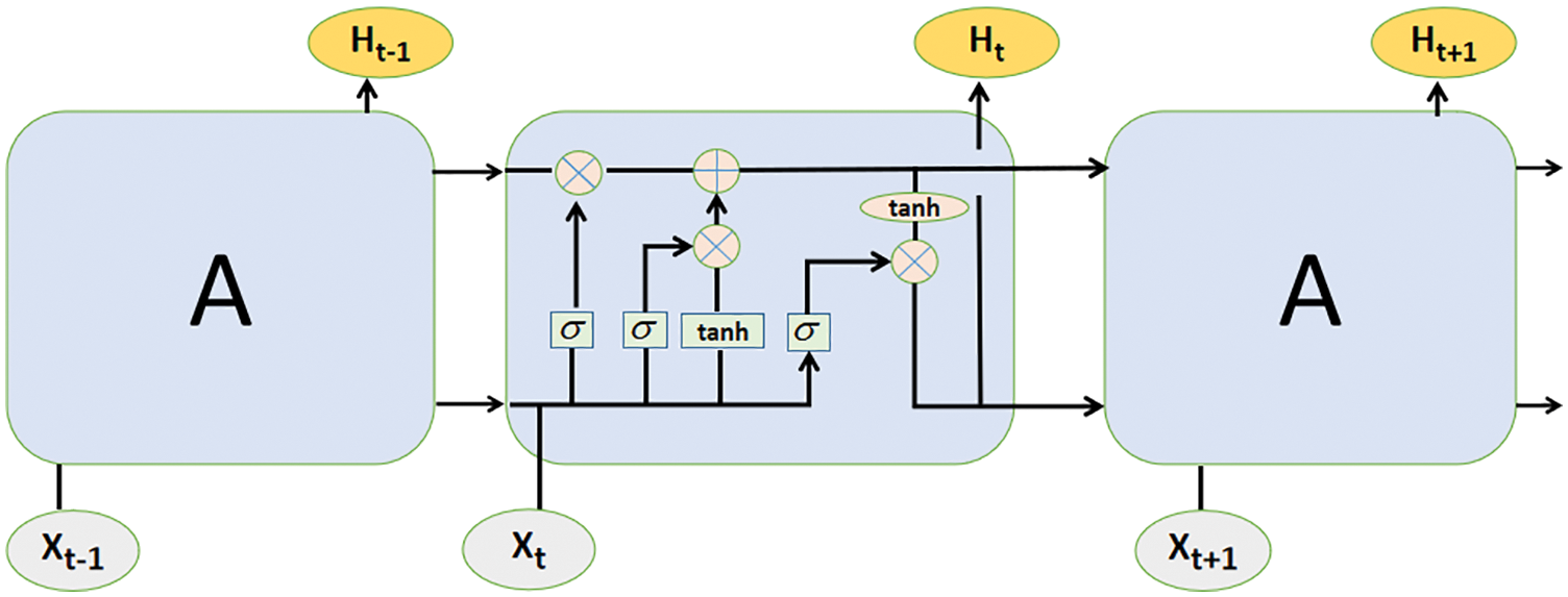
Figure 1: LSTM network structure
In the LSTM network, each LSTM module consists of an input gate i, an output gate o, a forgetting gate f, and a cell state c. The forget gate mainly determines which information to forget from the cell state; the input gate is to update which information from the cell state; and the output gate is to determine which information to output from the cell state, and the entire storage unit can be expressed by the following formula:
where, Ht is the hidden state at time t; Ct is the tuple state at time t; Xt is the input at time t; Ht − 1 is the hidden state at t − 1 moment, and the hidden state at the initial moment is 0. it, ft, gt, and ot are input gate, forget gate, select gate and output gate respectively; Sigma represents the Sigmoid activation function. In the transmission process of each unit, ct is usually ct−1 transferred from the previous state plus some values, which changes slowly, while ht has a wide range of values, so different nodes will have great differences [30]. LSTM’s processing of time series is mainly divided into three stages:
(1) Forgetting stage. This stage is mainly to selectively forget the input sequence of the previous node, which will “forget the unimportant and remember the important information”. That is, the value of ft is used to control what needs to be remembered and what needs to be forgotten in the previous state ct−1.
(2) Selecting the memory stage. In this stage, the input sequence Xt is selectively “remembered”. The input of the current unit is the calculated it, which can be selectively output by gt.
(3) Output stage. This phase determines which states will be considered as outputs of the current state, controlled primarily by ot, and scaled on ct using the tanh activation function.
3 Design of a CNN-LSTM Neural Network Model
3.1 Forecasting Framework Designing
In this paper, the water quality monitoring data set is constructed by a web crawler, and the dissolved oxygen concentration prediction model is constructed by CNN-LSTM hybrid network. The schematic block diagram is shown in Fig. 2. The model consists of three modules: data output layer, hidden processing layer, and prediction result output layer. The main function of the data input layer is the construction of water quality monitoring big data and data preprocessing. The hidden processing layer mainly extracts the data space through CNN and further extracts the time series features of the data from the spatial features of the data through LSTM. The prediction result layer mainly uses the fully connected layer to connect each node with all the data features output by the LSTM unit to realize the integration of local features and finally output the water quality prediction result.
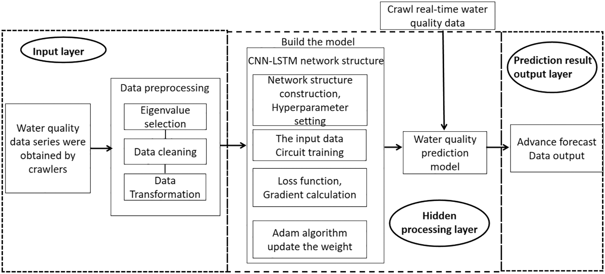
Figure 2: Water quality prediction scheme
3.2 CNN-LSTM Network Model Constructing
The changes of water quality data with time show a certain periodicity, and will be affected by other external factors, which makes the data change nonlinearly. Therefore, it is difficult to directly predict changes in water quality. Using the LSTM model alone for prediction can affect the maximum and minimum values of the data results, introducing noise that is not relevant to the prediction. Using the CNN model alone can lead to an overfitting problem caused by the excessive proportion of parameters in the whole connection layer [31,32]. Combining the advantages of CNN and LSTM network structure, the two models can be combined to form a CNN-LSTM model, which can better improve the accuracy of the model prediction effect. The CNN-LSTM model is shown in Fig. 3.
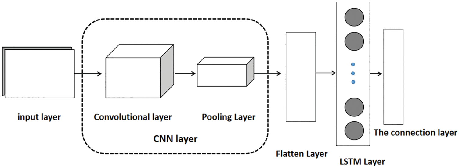
Figure 3: CNN-LSTM network structure
As can be seen from that in Fig. 3, the first part of the CNN-LSTM model is a CNN layer consisting of convolutional layers and max pooling layers. The convolution layer will traverse the water quality information transferred from the input layer, and use the weight of the convolution kernel to perform a convolution operation with the local sequence of the imported water quality information, Thereby a preliminary matrix with a higher expressive ability than the original sequence will be obtained. The new matrix obtained is used as input in the max pooling layer, and the pooling window is used to slide on the matrix sequence, and the maximum value of the window after each sliding is taken for pooling, thereby outputting a more expressive feature matrix. The stacked part is passed to the LSTM network through the Flatten layer, and the characteristics of the forget gate and the output gate of the LSTM model are used to filter and update the associated data information.
Some commonly used evaluation indexes include mean square error (MSE), root mean square error (RMSE), mean absolute percentage error (MAPE), Pearson correlation coefficient (PCC) [33,34], which can well reflect the actual situation of the error of the predicted value.
MSE is used to monitor the deviation between the predicted value and the actual value. It is an index to evaluate the performance of neural networks. The calculation formula of MSE is:
RMSE reflects the dispersion degree of systematic error and represents the deviation range between the predicted value and the real value. Different from MSE, MSE will change the dimension in the operation process, so the influence of dimension can be eliminated through RMSE. The larger the value of RMSE, the stronger the data volatility. The calculation formula of RMSE is:
MAPE reflects the ratio of actual error to the actual value, and essentially considers the ratio of actual error to the actual value. Its function is to use the same data to predict different models. The smaller the MAPE of the model prediction, the model will be better. The calculation formula of MAPE is:
Pearson correlation coefficient (PCC) is used to evaluate the correlation between real and predicted values. The closer the Pearson correlation coefficient is to 1, the better the restoration effect is. The calculation formula of PCC is:
where: xi is the measured value; xi′ is the predicted value of the model output; i is the sample number; n is the number of samples.
4 Experimental Results and Discussions
4.1.1 Water Quality Monitoring Data Set Constructing
The water quality monitoring data are from China National Environmental Monitoring Station (http://www.cnemc.cn/). By clicking on the national water quality automatic monitoring link, you can enter the water quality monitoring platform, as shown in Fig. 4. Water quality information mainly consists of site location, monitoring type, and monitoring time. Site locations include the province where the station is located, the watershed, and the section name. The monitoring types include water temperature, conductivity, dissolved oxygen, turbidity, permanganate index, ammonia nitrogen, total phosphorus, and total nitrogen. Monitoring time shows data updated in the last four hours.
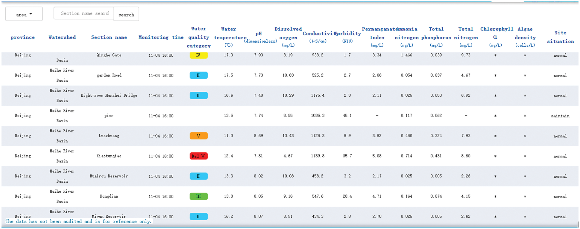
Figure 4: Water quality monitoring platform
When we enter the water quality monitoring platform, we can find that the data on this page is loaded dynamically. Therefore, if a crawler directly requests the uniform resource locator (URL) of the current interface, the returned hypertext markup language (HTML) is only the source code of the current interface, not the complete source code of all interfaces. There are usually two ways to crawl data for web pages that dynamically load data. One is to analyze the data interface of dynamically loaded data and convert it to a Python object by reading the JavaScript object notation (JSON) format string from the file. The second method is to load the web page and parse the rendered source code using selenium and browser to simulate the habits of natural people. Because the second method consumes central processing unit (CPU) and memory and is slow and slow in performance, this paper uses the first method to read JSON format string from a file and convert it to a python object to process the data. By going into developer mode, we can view the web page’s source code and related files and analyze the data interface for dynamically loading data.
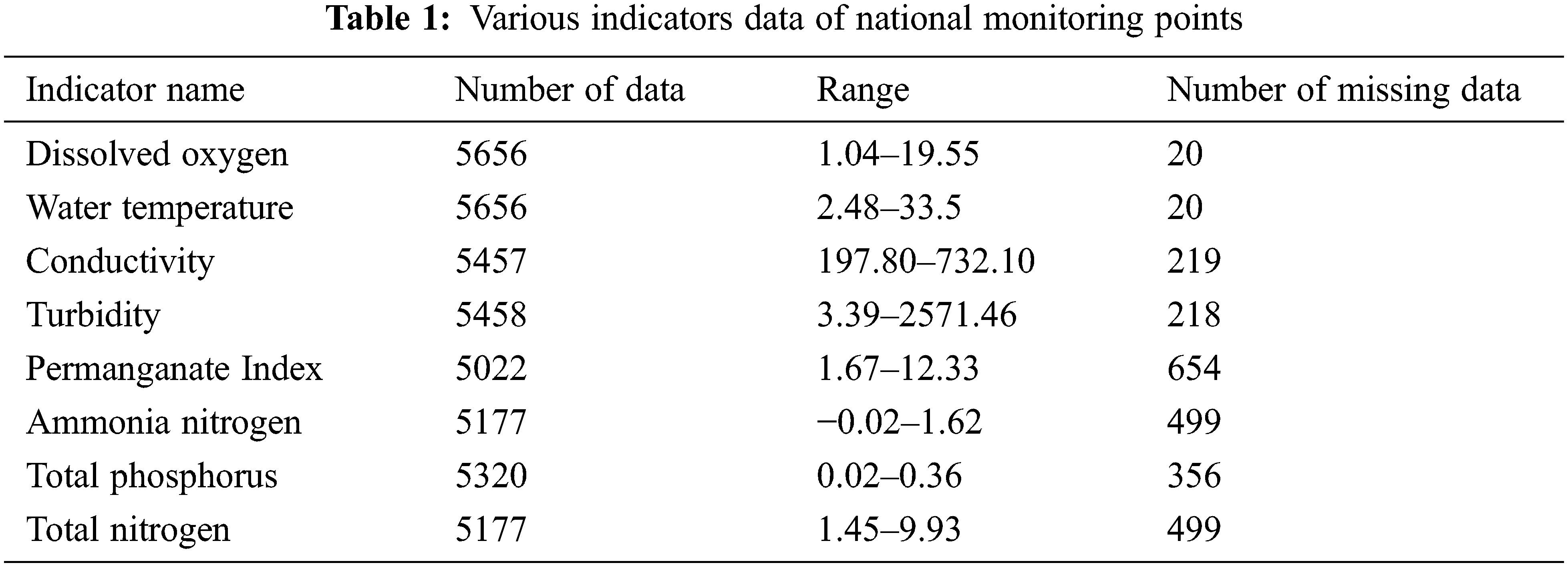
After extracting the required form through the POST request method, all the information could be crawled by changing the Pageindex and the PageSize. After analyzing the crawling data, a total of 5676 water quality monitoring data in the past three years, from July 1, 2018, to January 31, 2021, were summarized. The sorted data are shown in Tab. 1.
With the advent of the era of big data, the clutter, complexity, and fuzziness of raw data make the data processing face huge challenges in many aspects such as perception and calculation [35]. Data preprocessing is a very important preparatory work before data analysis and mining. On the one hand, it can ensure the accuracy and validity of the data; on the other hand, it can better meet the needs of data mining by adjusting the data format [36].
Data preprocessing comprises three parts: feature selection, data cleaning, and data conversion. The flow chart is shown in Fig. 5. Feature selection analyzes water quality characteristics and selects appropriate water quality characteristics for analysis; data cleaning mainly includes processing missing data, filtering outliers, and eliminating duplicate values; data transformation is performed by normalizing data.
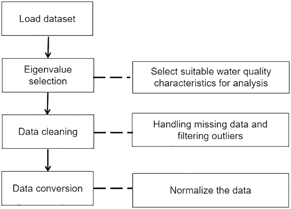
Figure 5: Data cleaning process
(1) Selection of eigenvalues. By observing the number of missing values in each indicator data of national monitoring sites in Tab. 1, it can be seen that the missing value of dissolved oxygen index in this area is the least, and the prediction of this index by using the prediction model has higher accuracy and reliability. Therefore, the dissolved oxygen will be taken as the primary research object to evaluate the water quality of this region.
(2) Missing value handling. The causes of the missing value [37] are broadly divided into human and natural factors. The natural factor is that in the process of data collection, due to machine factors, some of the data collection failed, or the collected data could not be stored, resulting in a section of data could not be saved. Human factors are due to human errors in the collection process, resulting in the omission of some data. When there are enough samples in the dataset, the ratio of missing values is relatively small. This small number of missing values has less impact on the whole situation and can be directly eliminated. Therefore, the missing data values are deleted directly in this experiment.
(3) Outliers handling. In the process of data collection, there will be abnormal objects due to different types of data sources, data measurement, and collection errors. Abnormal objects are often called outliers. Outlier detection, also known as deviation detection and exception mining, is often used as an important part of data mining. Its task is to find objects significantly different from most data. Therefore, most data mining methods treat this difference information as noise [38]. The boxplot uses the distance between the interquartile values as the basis for judgment, so the boxplot has objectivity and superiority in identifying outliers. It can be seen from the obtained data set that there are exaggerated data between the maximum and minimum values of dissolved oxygen, which may be due to the long working time of the instrument and the aging of the instrument, resulting in errors in the data at some time points. Therefore, these data can be regarded as abnormal values during data analysis. The effect of eliminating abnormal values in the box diagram is shown in Fig. 6, and the comparison diagram after handling the abnormal values of dissolved oxygen is shown in Fig. 7.
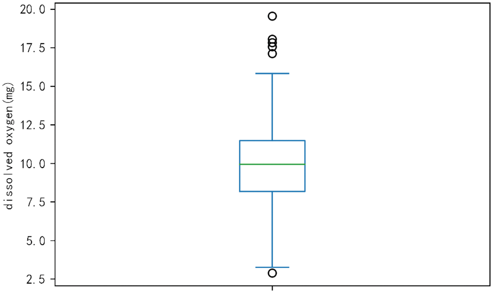
Figure 6: Dissolved oxygen outliers box plot
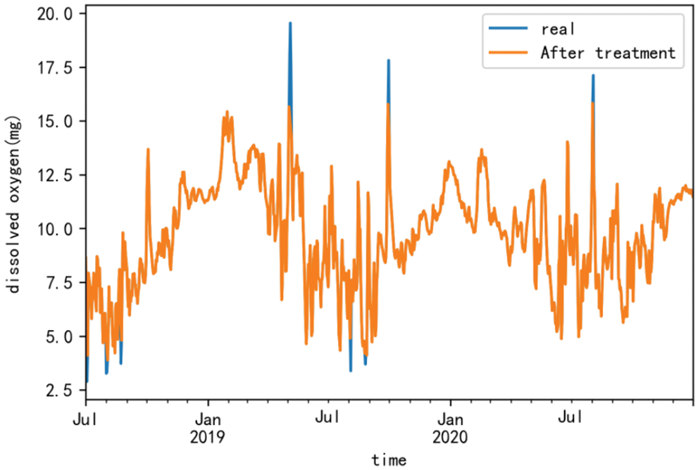
Figure 7: Comparison of dissolved oxygen outlier treatment
(4) Normalization. In order to make CNN-LSTM model converge faster and have higher stability in the training process, the data of dissolved oxygen are normalized to make the dissolved oxygen data between [0,1]. The normalization formula is:
(5) Data dividing. In order to prevent the model from performing well in the training set but generally in the test set, the generalization ability is weak. Therefore, this paper resamples 915 data of dissolved oxygen concentration in chronological order by day and divides the data into training set and verification set in the proportion of 8:2 in the process of training. That is, 732 sample data from July 1, 2018, to July 1, 2020, are used for model training, and 183 sample data from July 2, 2020, to January 31, 2021, are used to verify the performance of the model.
(6) Data restoring. When evaluating the model after training, to eliminate the impact of normalization on the prediction results, the predicted data needs to be restored to evaluate the error of the model’s predicted value. The inverse normalization formula is:
The CNN-LSTM model is mainly composed of the input layer, convolution layer, pooling layer, LSTM layer, fully connected layer, and output layer. In the windows environment, the deep learning library Keras 2.3.1 is used to build a neural network model. Google’s open-source artificial intelligence system Tensorflow1.1.0 is used as the back-end computing framework. Because adaptive motion estimation (Adam) has the advantages of fast convergence and better learning ability, the prediction models in this paper are trained by using Adam’s optimization algorithm and learning rate of 0.001. At the same time, to reduce the influence of human factors on the prediction model, we complete 100 epochs (one epoch means traversing all samples in a training set) to obtain the parameters of the CNN-LSTM model.
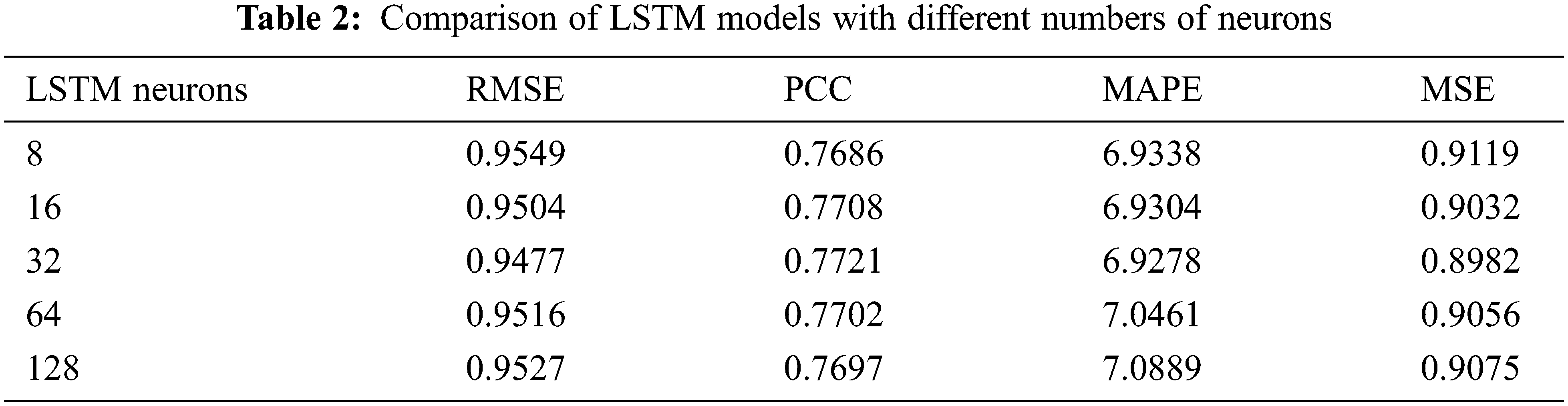
The construction of the model consists of two parts: the construction of the LSTM model and the construction of the CNN model. The first part is the determination of LSTM model parameters. To determine the most appropriate number of neurons, we need to put the test set data into the LSTM model for training. From Tab. 2, we can see that when the number of neurons in the LSTM layer is 32, the values of the four indicators are at the best value, and the accuracy and stability of the LSTM model are the best.
The second part is the determination of CNN model parameters. Because the CNN-LSTM prediction model uses the data extracted from the features of convolution layer and pooling layer as the input of LSTM. It is necessary to determine the parameters of the CNN convolution layer and pooling layer when determining the LSTM parameters. However, the size and number of various convolution kernels will also affect the actual effect. Therefore, this paper sets the number of convolution cores as four groups (8, 16, 32, 64) and the size of convolution cores as three groups (1, 2, 3). When the number of convolution cores is fixed, the effects of different convolution core sizes on the four prediction indexes are tested, and the parameter configuration and model evaluation index values are shown in Tab. 3.
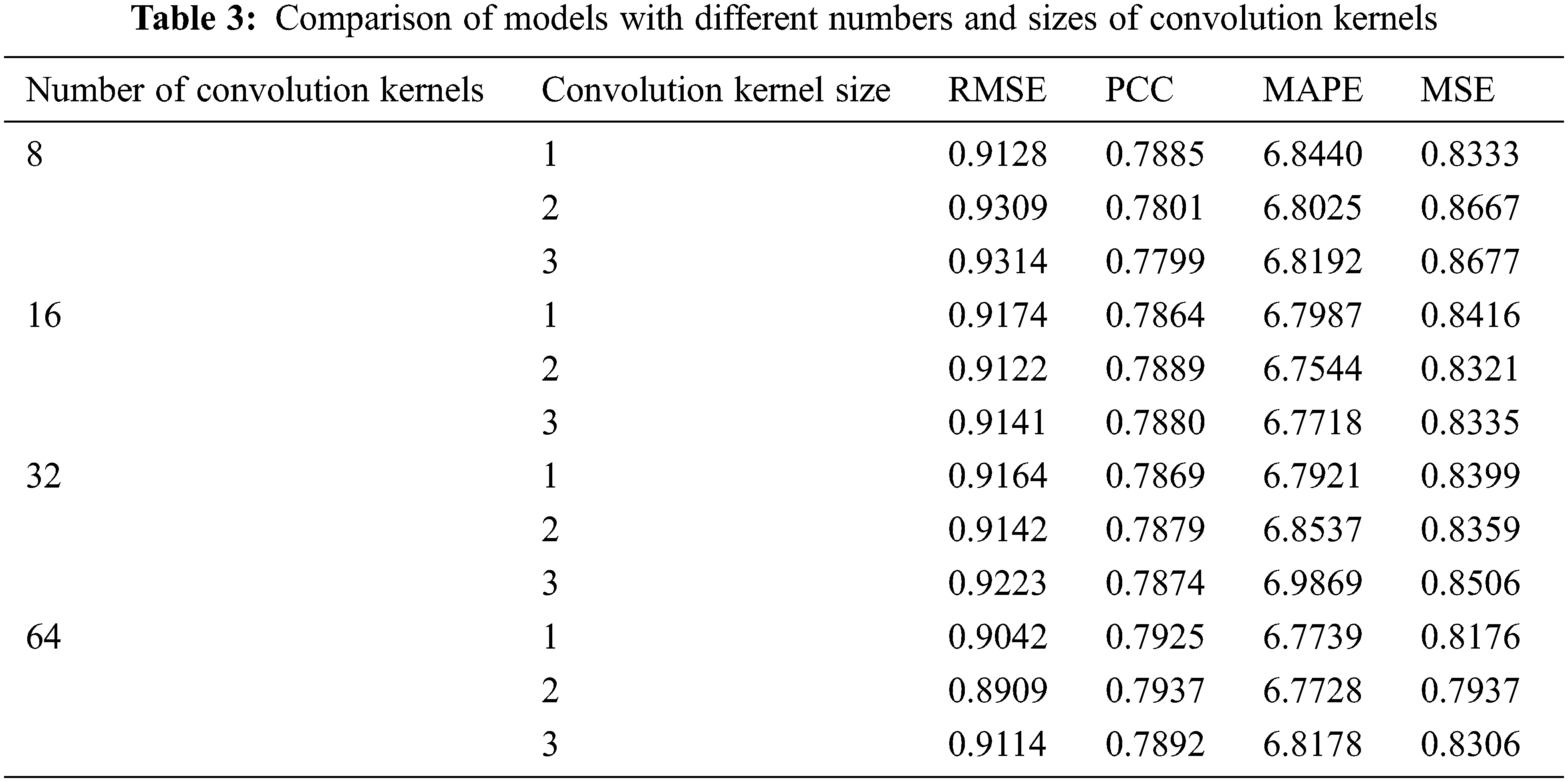
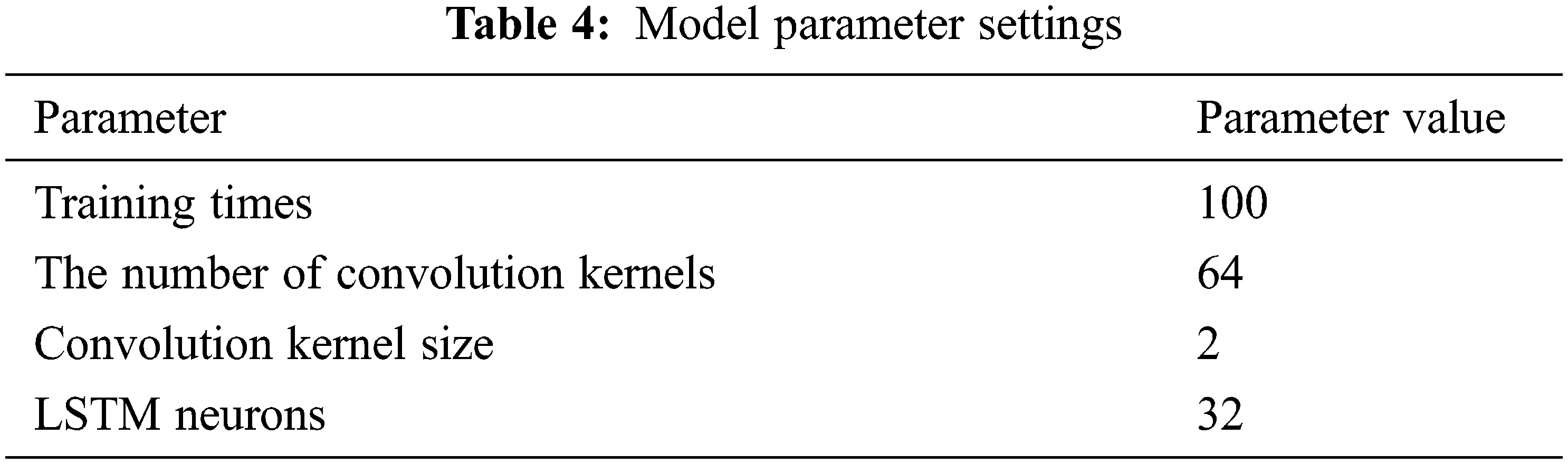
It can be seen from Tab. 3 that when the number of convolution kernels in the convolutional layer is 64, and the convolution kernel size is 2, the prediction performance of the CNN-LSTM model is the best. Combined with the above experimental training, some model parameter settings are shown in Tab. 4.
The change curve of the loss function of the proposed CNN-LSTM model is shown in Fig. 8. It can be seen from the figure that with the continuous increase of the number of iterations in the training process, the loss curve of the samples in the training set decreases significantly at first and then tends to stabilize. When the number of iterations reaches more than 40 times, the loss function becomes a straight line parallel to the x-axis, and finally, the expected model is obtained.
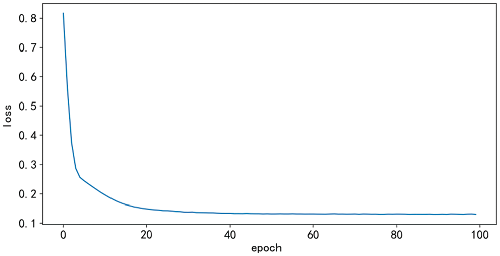
Figure 8: The loss function curve of the model
In order to compare the prediction effect of the two models on the actual data, this experiment uses the LSTM model and the CNN-LSTM model to predict the dissolved oxygen concentration in the test sample respectively. At the same time, in order to more clearly compare the prediction effects of the two models, we performed a visual comparative analysis of the first 100 samples, as shown in Figs. 9 and 10. It can be seen from the figure that although LSTM can better predict the periodic change of dissolved oxygen, the fitting between the more significant value and the smaller value is relatively poor, resulting in relative deviation. However, CNN-LSTM not only inherits the ability of LSTM to remember and forget the previous data of time series, but also solves the problem of inaccurate prediction of large and small values by LSTM and has a better fitting effect on the peak value. It can be shown that CNN-LSTM has a more robust prediction performance.

Figure 9: Prediction curves for the LSTM model
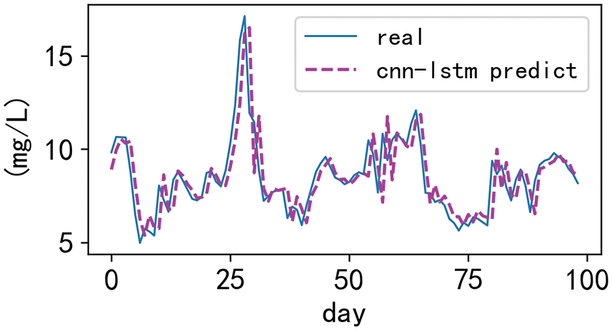
Figure 10: Prediction curves for the CNN-LSTM model
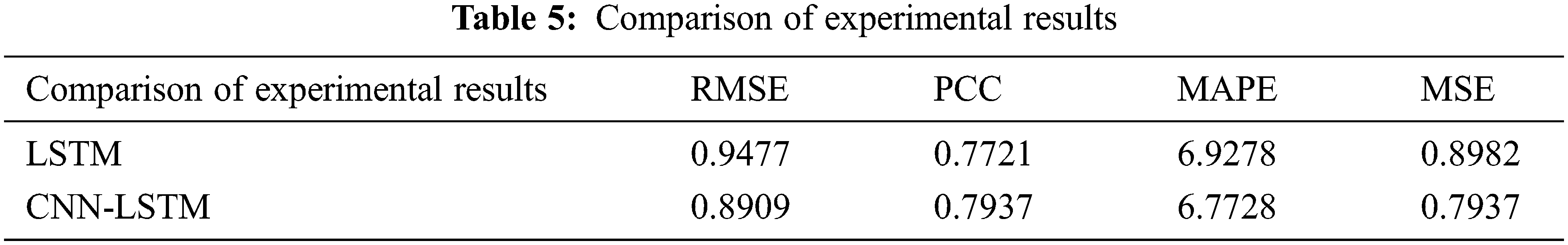
The four evaluation metrics MAPE, PCC, MSE, and RMSE of the CNN-LSTM model and LSTM model are shown in Tab. 5. Compared with the original LSTM prediction model, CNN-LSTM, improves the four evaluation indicators to a certain extent. The RMSE of the hybrid model is 5.99% lower than that of the single model, the PCC is increased by 2.80%, the MAE is reduced by 2.24%, and the MSE is reduced by 11.63%.
In order to solve the problem of too many influencing factors and difficult prediction of water quality change, this paper proposed a CNN-LSTM combined model to forecast the dissolved oxygen data in water quality. In this model, the data features extracted by CNN can be stored in LSTM for long-term memory, highlighting the role of these data features in the prediction process, thus improving the accuracy of the model. Compared with the traditional LSTM model, the RMSE, PCC, MAE, and MSE respectively improved by 5.99%, 2.80%, 2.24%, and 11.63%. The drawbacks of the proposed method include too few selection factors and only considering the iterative method to solve the above tasks. With this in mind, the further research is necessary, including the following:
(1) More input variables will be added to optimize the prediction model further. A multi-layer hidden layer will be used to improve the accuracy of the prediction of dissolved oxygen concentration.
(2) Non-iteration methods will be used to incorporate the model, which further improves the accuracy of the model prediction [39,40].
(3) While adding more input variables, some independent variables are related to each other so that we can eliminate collinearity by principal component analysis.
Acknowledgement: The authors would like to appreciate all anonymous reviewers for their insightful comments and constructive suggestions to polish this paper in high quality.
Funding Statement: This research was funded by the National Natural Science Foundation of China (No. 51775185), Natural Science Foundation of Hunan Province, Scientific Research Fund of Hunan Province Education Department (18C0003), Research project on teaching reform in colleges and universities of Hunan Province Education Department (20190147), and Hunan Normal University University-Industry Cooperation. This work is implemented at the 2011 Collaborative Innovation Center for Development and Utilization of Finance and Economics Big Data Property, Universities of Hunan Province, Open project, Grant Number 20181901CRP04.
Conflicts of Interest: The authors declare that they have no conflicts of interest to report regarding the present study.
1. Y. M. Wang, “Interpretation of the current situation of surface water quality monitoring in China,” Theoretical Research on Urban Construction (Electronic Edition), vol. 9, no. 15, pp. 120, 2019. [Google Scholar]
2. Y. T. Xiao, J. Zhang, M. Wu, H. Liu, D. Zhang et al., “Research on water pollution and drinking water safety in China,” Resources and Environment in the Yangtze Basin, vol. 10, no. 1, pp. 51–59, 2001. [Google Scholar]
3. S. J. Ma and B. L. Gao, “Analysis of the status quo and countermeasures of surface water quality monitoring,” Jiangsu Science and Technology Information, vol. 34, no. 11, pp. 38–39, 2017. [Google Scholar]
4. M. Li, “Research progress of aerobic denitrifying biological nitrogen removal technology,” Guangdong Chemical, vol. 42, no. 13, pp. 119–120, 2015. [Google Scholar]
5. X. Q. Yin, “Analysis of dissolved oxygen variation law and influencing factors in Mangjou reservoir,” Environmental Science Guide, vol. 40, no. 1, pp. 56–58, 2021. [Google Scholar]
6. J. Zhang, Y. Sheng, W. Chen, H. Lin, G. Sun et al., “Design and analysis of a water quality monitoring data service platform,” Computers, Materials & Continua, vol. 66, no. 1, pp. 389–405, 2021. [Google Scholar]
7. G. Sun, F. H. Li and W. D. Jiang, “Brief talk about big data graph analysis and visualization,” Journal on Big Data, vol. 1, no. 1, pp. 25–38, 2019. [Google Scholar]
8. B. Yang, L. Xiang, X. Chen and W. Jia, “An online chronic disease prediction system based on incremental deep neural network,” Computers, Materials & Continua, vol. 67, no. 1, pp. 951–964, 2021. [Google Scholar]
9. Y. Sheng, J. Zhang, W. Tan, J. Wu, H. Lin et al., “Application of grey model and neural network in financial revenue forecast,” Computers, Materials & Continua, vol. 69, no. 3, pp. 4043–4059, 2021. [Google Scholar]
10. W. D. Jiang, J. Wu, G. Sun, Y. X. Ouyang, J. Li et al., “A survey of time series data visualization methods,” Journal of Quantum Computing, vol. 2, no. 2, pp. 105–117, 2020. [Google Scholar]
11. Y. K. Hu, N. Wang, S. Liu, Q. L. Jiang and N. Zhang, “Application research of time series model and LSTM model in water quality prediction,” Small Microcomputer System, vol. 42, no. 8, pp. 1569–1573, 2021. [Google Scholar]
12. C. W. Xiong, “Improvement of ant colony algorithm and its application in path planning,” M.S. Dissertation, Chongqing University of Posts and Telecommunications, Chongqing, 2020. [Google Scholar]
13. Y. C. Le, Y. Bengio and G. Hinton, “Deep learning,” Nature, vol. 521, no. 7553, pp. 436–444, 2015. [Google Scholar]
14. G. Reshma, C. Atroshi, V. K. Nassa, B. Geetha, G. Sunitha et al., “Deep learning-based skin lesion diagnosis model using dermoscopic images,” Intelligent Automation & Soft Computing, vol. 31, no. 1, pp. 621–634, 2022. [Google Scholar]
15. L. Y. Liu, J. He, K. Y. Ren, J. Lungu, Y. B. Hou et al., “An information gain-based model and an attention-based RNN for wearable human activity recognition,” Entropy, vol. 23, no. 12, pp. 1635–1635, 2021. [Google Scholar]
16. L. Xiang, G. Guo, Q. Li, C. Zhu, J. Chen et al., “Spam detection in reviews using LSTM-based multi-entity temporal features,” Intelligent Automation & Soft Computing, vol. 26, no. 6, pp. 1375–1390, 2020. [Google Scholar]
17. Y. Z. Wei and X. N. Xu, “Ultra-short-term wind speed prediction based on LSTM long short-term memory network,” Journal of Electronic Measurement and Instrumentation, vol. 33, no. 2, pp. 64–71, 2019. [Google Scholar]
18. Z. Yan, C. C. Yu and L. Han, “Short-term traffic flow prediction method based on CNN + LSTM,” Computer Engineering and Design, vol. 40, no. 9, pp. 2620–2624, 2019. [Google Scholar]
19. J. X. Lu, Q. P. Zhang, Z. H. Yang, Y. B. Hou and R. H. Dong, “Short-term load forecasting method based on CNN-LSTM hybrid neural network model,” Automation of Electric Power Systems, vol. 43, no. 8, pp. 131–137, 2019. [Google Scholar]
20. Y. Wang, X. N. Feng and T. Y. Qian, “Intrusion detection of camouflaged users based on CNN and LSTM deep network,” Computer Science and Exploration, vol. 12, no. 4, pp. 575–585, 2018. [Google Scholar]
21. K. Kumar and M. T. U. Haider, “Enhanced prediction of intra-day stock market using metaheuristic optimization on RNN–LSTM network,” New Generation Computing, vol. 39, no. 1, pp. 231–272, 2021. [Google Scholar]
22. T. Li, M. Wu and X. Wu, “A hybrid CNN-LSTM model for forecasting particulate matter (PM2.5),” IEEE Access, vol. 8, pp. 26933–26940, 2020. [Google Scholar]
23. Y. C. Mao, T. Y. Chen, H. S. Chou, S. Y. Lin, S. Y. Liu et al., “Caries and restoration detection using bitewing film based on transfer learning with CNNs,” Sensors, vol. 21, no. 13, pp. 4613, 2021. [Google Scholar]
24. M. Geravanchizadeh and H. Roushan, “Dynamic selective auditory attention detection using RNN and reinforcement learning,” Scientific Reports, vol. 11, no. 1, pp. 1–11, 2021. [Google Scholar]
25. S. Hochreiter and J. Schmidhuber, “Long short-term memory,” Neural Computation, vol. 9, no. 8, pp. 1735–1780, 1997. [Google Scholar]
26. R. Chandra and A. Jain, “Deep learning via LSTM models for COVID-19 infection forecasting in India,” PLoS One, vol. 17, no. 1, pp. 1–28, 2022. [Google Scholar]
27. X. Wang, J. Wu, C. Liu, H. Y. Yang, Y. L. Du et al., “Fault time series prediction based on LSTM recurrent neural network,” Journal of Beijing University of Aeronautics and Astronautics, vol. 44, no. 4, pp. 772–784, 2018. [Google Scholar]
28. R. Xu, “Research and application of water quality prediction method in beilun estuary based on SARIMA-LSTM,” M.S. Thesis, Chongqing University, Chongqing, 2019. [Google Scholar]
29. F. Li, Y. Chen and W. Xiang, “State degradation trend prediction based on quantum weighted long-short term memory neural network,” Chinese Journal of Scientific Instrument, vol. 39, no. 7, pp. 217–225, 2018. [Google Scholar]
30. M. J., Hamayel and A. Y. Owda, “A novel cryptocurrency price prediction model using GRU, LSTM and bi-LSTM machine learning algorithms,” AI, vol. 2, no. 4, pp. 477–496, 2021. [Google Scholar]
31. J. Wang, Z. X. Gao and Y. M. Zhu, “Research on water quality prediction of Yellow River based on CNN-LSTM model,” People’s Yellow River, vol. 43, no. 5, pp. 96–99, 2021. [Google Scholar]
32. J. Kim, J. Choe and K. Lee, “Sequential field development plan through robust optimization coupling with CNN and LSTM-based proxy models,” Journal of Petroleum Science and Engineering, vol. 209, pp. 109887, 2022. [Google Scholar]
33. L. Germánico and A. Pablo, “Short-term wind speed forecasting over complex terrain using linear regression models and multivariable LSTM and NARX networks in the Andes mountains, Ecuador,” Renewable Energy, vol. 183, pp. 351–368, 2022. [Google Scholar]
34. H. Y. Wu, Y. P. Cai, Y. S. Wu, P. Zhong, Q. Li et al., “Time series analysis of weekly influenza-like illness rate using a one-year period of factors in random forest regression,” Bioscience Trends, vol. 11, no. 3, pp. 292–296, 2017. [Google Scholar]
35. S. Y. Yin, X. K. Chen and L. Shi, “Python-based data desensitization and visual analysis,” Computer Knowledge and Technology, vol. 15, no. 6, pp. 14–17, 2019. [Google Scholar]
36. Q. Sun, C. Q. Ye and Y. Sun, “Research on data preprocessing methods under big data,” Computer Technology and Development, vol. 28, no. 5, pp. 1–4, 2018. [Google Scholar]
37. W. J. Zhang, “Research on personal credit risk assessment model based on big data,” Ph.D. Dissertation, University of International Business and Economics, Beijing, 2016. [Google Scholar]
38. W. B. Deng, “Research on dominant relation rough set method for uncertain information processing,” Ph.D. Dissertation, Southwest Jiaotong University, Chengdu, 2015. [Google Scholar]
39. I. Izonin, R. Tkachenko, V. Verhun and K. Zub, “An approach towards missing data management using improved GRNN-SGTM ensemble method,” Engineering Science and Technology, an International Journal, vol. 24, no. 3, pp. 749–759, 2021. [Google Scholar]
40. R. Tkachenko, I. Izonin, I. Dronyuk, M. Logoyda and P. Tkachenko, “Recovery of missing sensor data with GRNN-based cascade scheme,” International Journal of Sensors Wireless Communications and Control, vol. 11, no. 5, pp. 531–541, 2021. [Google Scholar]
 | This work is licensed under a Creative Commons Attribution 4.0 International License, which permits unrestricted use, distribution, and reproduction in any medium, provided the original work is properly cited. |