Intelligent Automation & Soft Computing DOI:10.32604/iasc.2022.026385
Article

Convolutional Neural Networks Based Video Reconstruction and Computation in Digital Twins

M. Kavitha1, B. Sankara Babu2, B. Sumathy3, T. Jackulin4, N. Ramkumar5, A. Manimaran6, Ranjan Walia7 and S. Neelakandan8,*

1Department of Computer Science and Engineering, Vel Tech Rangarajan Dr. Sagunthala R&D Institute of Science and Technology, Chennai, 600 062, India
2Department of Computer Science and Engineering, Gokaraju Rangaraju Institute of Engineering and Technology, Hyderabad, 500 090, India
3Department of Instrumentation and Control Engineering, Sri Sairam Engineering College, Chennai, 602 109, India
4Department of Computer Science and Engineering, Panimalar Engineering College, Chennai, 600 123, India
5Department of Statistics, Vishwakarma University, Pune, 411 048, India
6Department of Computer Applications, Madanapalle Institute of Technology & Science, Madanapalle, 517 325, India
7Department of Electrical Engineering, Model Institute of Engineering and Technology, Jammu, 181 122, India
8Department of Computer Science and Engineering, R.M.K Engineering College, Kavaraipettai, 601 206, India
*Corresponding Author: S. Neelakandan. Email: snksnk17@gmail.com
Received: 24 December 2021; Accepted: 27 January 2022

Abstract: With the advancement of communication and computing technologies, multimedia technologies involving video and image applications have become an important part of the information society and have become inextricably linked to people's daily productivity and lives. Simultaneously, there is a growing interest in super-resolution (SR) video reconstruction techniques. At the moment, the design of digital twins in video computing and video reconstruction is based on a number of difficult issues. Although there are several SR reconstruction techniques available in the literature, most of the works have not considered the spatio-temporal relationship between the video frames. With this motivation in mind, this paper presents VDCNN-SS, a novel very deep convolutional neural networks (VDCNN) with spatiotemporal similarity (SS) model for video reconstruction in digital twins. The VDCNN-SS technique proposed here maps the relationship between interconnected low resolution (LR) and high resolution (HR) image blocks. It also considers the spatiotemporal non-local complementary and repetitive data among nearby low-resolution video frames. Furthermore, the VDCNN technique is used to learn the LR–HR correlation mapping learning process. A series of simulations were run to examine the improved performance of the VDCNN-SS model, and the experimental results demonstrated the superiority of the VDCNN-SS technique over recent techniques.

Keywords: Digital twins; video reconstruction; video computation; multimedia; deep learning; curvelet transform

1  Introduction

Over the last few decades, multimedia has become an increasingly important component of people's daily life. It is used as a result of the rapid development of internet users, which, according to ITU (International Telecommunication Union) figures, reached approximately 3.2 billion users in 2015 [1,2]. Alternatively, the purchasing cost of multimedia capturing devices is decreasing, and the majority of the devices are now embedded in tablet, laptop, and mobile phone, making media production a work that can be completed by anybody, at any time and from any location [3]. Finally, the influence of social media and the human desire to interact with family and friends through chatting, words, and texts, as well as the richness of audio-visual content, has inspired a novel way of communicating with their social surroundings via social networks such as Twitter, Facebook, and Instagram [4]. As a result, the diversity, amount, and complexity of digital media generated, recorded, analysed, saved, and processed via distributed and heterogeneous media sources and cloud frameworks such as Flickr and Picasa have increased. This vast amount of multimedia content, known as User Generated Content (UGC) [5] could be used to improve human-to-human communication, but it is also used in a variety of unique application domains such as culture, tourism, entertainment, and leisure. The general technique of video reconstruction is depicted in Fig. 1.

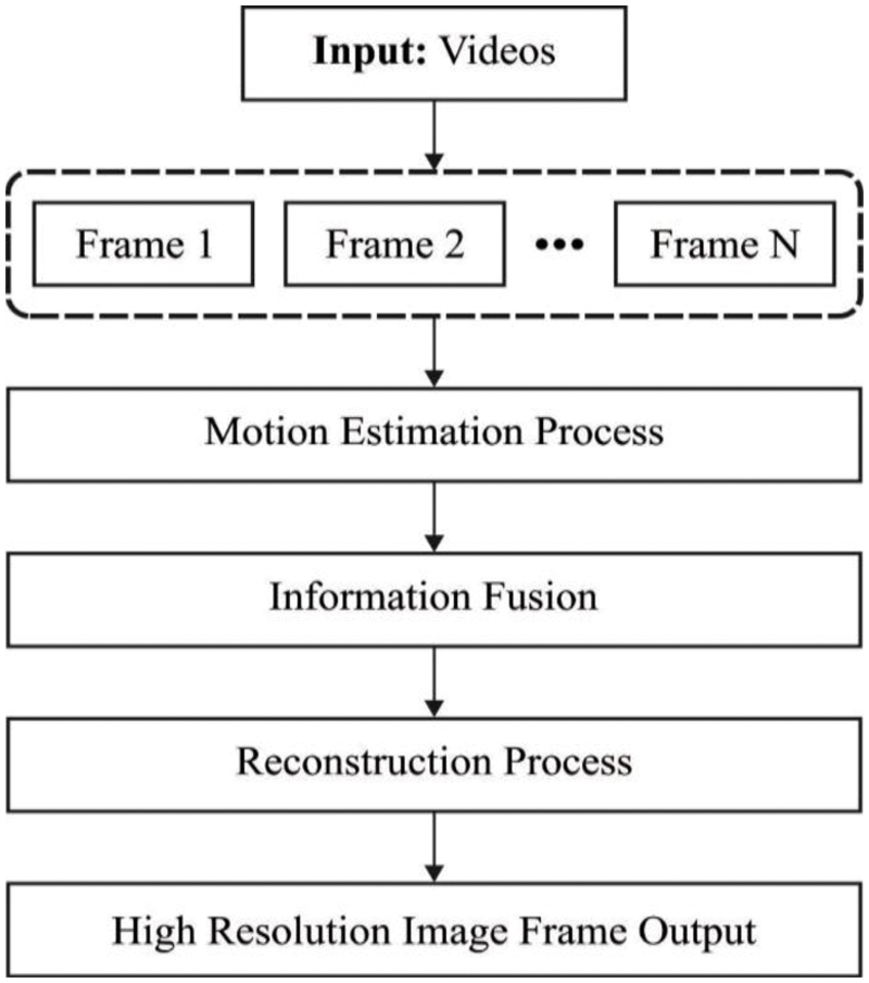
Figure 1: General video reconstruction process

One intriguing approach is to use today's massive multimedia data sources for the reconstruction step [6]. This will result in “wild” modelling, in which image data are obtained from distributed, web/social-based multimedia sources for private or other purposes but not for correct reconstruction [7]. They expanded on the preceding approach in this study by focusing on video series hosted on heterogeneous and dispersed multimedia platforms. The goal is to generate modules of the scene they portray using high visual data from video content. As a result, such movies contain a plethora of non-interesting items and noises, such as persons in front of a cluttered background, monuments, moving vehicles, and so on [8].

To create modules, the video frames are first summarized using a video summarizing algorithm. To summarise the videos, the unique idea proposed is to use discriminant Principal Component Analysis (d-PCA). Recently, the d-PCA concept [9] was proposed to cluster the objects in order to maximize the coherency of the foreground to the background. The use of Machine Learning (ML) based techniques is widespread in many aspects of their lives, ranging from corporate logistics and advertising schemes to applications on their cameras and smartphones, which are supported by a large number of devices and dedicated hardware. Recently, there has been a surge in interest in Deep Learning (DL) approaches in the research community. It is a subset of ML approaches that enables a smart scheme for manually learning an acceptable data representation from the data itself. Because of the potential of DL-based approaches for extracting the implicit data of this type of information, it is particularly beneficial for multimedia applications such as audio and video classifications. Many DL classifications, for example, have attained human performance in medical image classification for recognizing a large variety of disorders, narrowing the gap between machine and human analytical capacity.

Recently, deep learning techniques have produced efficient learning methods in a wide spectrum of AI, particularly for video and image analytics. This method can extract knowledge from massive amounts of unstructured data and deliver data-driven solutions. They have made significant progress in a wide range of research applications and domains, including pattern recognition, audio visual signal processing, and computer vision. Furthermore, it is expected that DL and its improved methodologies would be included into future image and sensor schemes. These methods are commonly used in CV and, more recently, video analysis. Indeed, different DL methods have emerged in research scholars, business, and academics scientists with efficient answers for numerous video and image-related difficulties. The primary goal of developing DL is to achieve greater detection accuracy than prior algorithms. With the rapid development of creative DL approaches and models such as Long Short-term Memory, Generative Adversarial Networks, DotNetNuke, and Recurrent Neural Network, as well as the increased demand for visual signal processing efficiency, unique probabilities are emerging in DL-based video processing, sensing, and imaging.

This research introduces VDCNN-SS, a novel VDCNN with spatiotemporal similarity (SS) model for video reconstruction in digital twins. The suggested VDCNN-SS technique visualizes the relationship between interconnected low resolution (LR) and high resolution (HR) picture blocks. It deals with non-local complementary and repeating data that is spatially and temporally distributed across nearby low-resolution video frames. The VDCNN model is utilized for learning the LR–HR correlation mapping to improve reconstruction speed while maintaining SR quality, and the resultant HR video frames are obtained effectively and quickly. A thorough simulation analysis is performed to evaluate the improved SR video reconstruction performance of the VDCNN-SS technique, and the findings are examined in terms of several evaluation factors.

2  Structure

Mur et al. [10] suggested a fast DL reconstructor that uses spatiotemporal information in a video. They were particularly interested in convolution gated recurrent units, which have lower memory requirements. These simulations show that the projected recurrent network improves reconstruction quality over static approaches that recreate video frames separately. Yao et al. [11] proposed a new DR2-Net for reconstructing the image from their CS measurement. The DR2-Net is based on two explanations: 1) Residual learning can improve reconstruction quality further, and 2) linear mapping can reconstruct higher quality primary pictures. As a result, DR2-Net has two modules: a residual network and a linear mapping network. The FC layer of NN, in particular, performs the linear mapping network.

Sankaralingam et al. [12] take advantage of learning-based algorithms in video SR fields, proposing a new video SR reconstruction approach based on Deep Convolutional Neural Networks and Spatio-Temporal Convolutional Neural Network-Super Resolution. It is a DL technique for reconstructing video SR that implies a mapping relationship between related HR and LR picture blocks, as well as redundant information and spatio-temporal non-local complements among neighbouring LR video frames. Sundaram et al. [13] presented a super-resolution (SR) reconstruction technique based on an effective subpixel CNN, whereas the optical flow is provided in the DL network. In addition, a superpixel convolutional layer is added after the DCN to improve the SR. Higham et al. [14] demonstrate the DL application employing convolution AE networks for recovering real-world 128128-pixel video at thirty frames per second from single pixel camera sampling at a compression ratio of 2%. Furthermore, by training the network on a large database of images, it optimizes the first layer of the convolution networks, which is equivalent to optimizing the basis used to scan the image intensities. Prakash et al. [15] asserts that by learning from an instance of a specific context, this method offers the possibility of HR for task-specific adaptation, which has implications for applications in metrology, gas sensing, and 3D imaging.

Kong et al. [16] used two DL modules to improve the spatial resolution of temperature regions. In MPSRC, the three pathways with and without pooling layers are targeted at fully reflecting the spatial distribution feature of temperature. The appropriate HR temperature regions have been successfully and accurately rebuilt. Judith et al. [17] investigate a new foveated reconstruction technique that makes use of recent advances in generative adversarial NN. They rebuilt a believable peripheral video from a smaller fraction of pixels that provided each frame. When it comes to providing a visual experience with no evident quality deterioration, this technology outperforms advanced foveated rendering.

3  The Proposed Video Reconstruction Model

This study developed a new VDCNN-SS technique for digital twins that employs correlation mapping between the outer correlative blocks and nonlocal paired and repetitive data in surrounding LR video frames to get higher quality reconstruction results. During the learning method, the VDCNN-SS technique employs the VDCNN model to get the reconstruction variables among the LR and HR picture blocks that increase the SR speed. In addition, curvelet transform (CLT) and structural similarity (SSIM) are used to provide spatiotemporal fuzzy registration and fusion across neighbouring frames at the subpixel level. At this point, the VDCNN-SS approach is extremely responsive to a complex motion process and produces robust results. The complete working process is represented in Fig. 2, which includes two primary processes: correlation mapping learning and SSIM measurement.

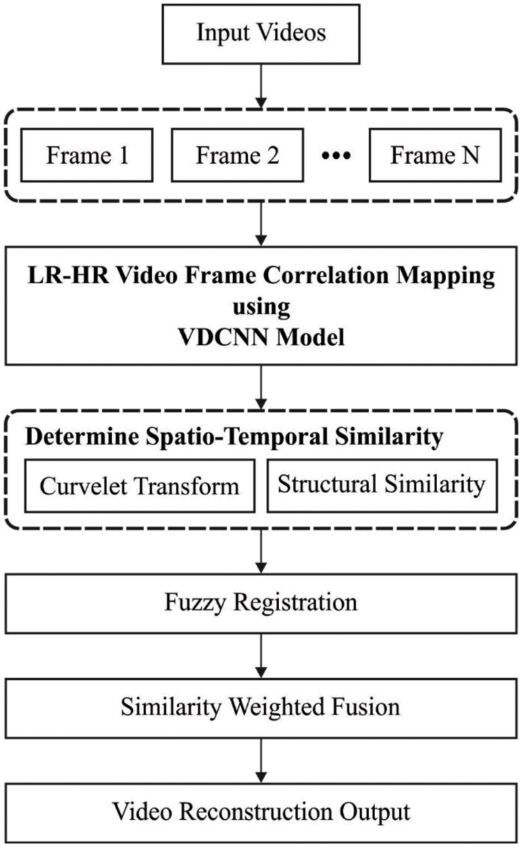
Figure 2: Overall process of VDCNN-SS model

3.1 Design of VDCNN Based Correlation Mapping Learning Model

Correlation mapping learning is a method for learning the relationships between HR and LR video frames. Sparse coding refers to the removal of all patches from the training set in order to reduce the burden of storage and computation. This approach comprises multiple parts, which are summarized below: reconstruction, patch extraction, sparse representation, and correlation mapping.

Fi(Y)=max(0,Wi∗Fi−1(Y)+Bi) (1)

Whereas {W,B}={W1,W2,W3,B1,B2,B3} denoted the filter and the bias attained during the training procedure. The index i denotes the NN layer in the reconstruction procedure, and if i = 0, F0( Y) signifies the input image which could be simply noted as X. Besides, the filter consist of 4 dimensional matrices and the bias consists of vector. In additional explanations, c is presented for denoting the channel of frame. fi and ni utilized for denoting the size and number of the filters in i layer, respectively. Later, they could utilize these functions for representing the succeeding 3 phases:

1)   Patch extraction and sparse depiction. The filter W1 dentoes the matrix of size c × f1 × f1 × n1 and bias B1 indicates an n1-dimension vector, whereas f1 & n1 denotes the size and amount of the filters in the initial layer. Eq. (1) could be considered as implementing n1 convolution on input frame X using a kernel sized c × f1 × f2 and output an n1-dimension vector.

2)   Correlation mapping. Here, the size of W2 is n1 × f2 × f2 × n2 and B2 denotes an n2-dimension vector, afterward implementing n2 convolution to F1(Y), they could map n1-dimension LR image block to n2-dimension HR image block.

3)   Reconstruction. Here, the size of W3 is n2 × f3 × f3 × c, B3 implies the c-dimensional vector and the output F3(Y) denotes a c-dimensional vector, that has the pixel value in the target area. Therefore, the HR frame is reconstructed using a VDCNN.

The VDCNN is an adaptive framework for identifying text processes that was designed to provide different depth levels (9, 17, 29, and 49). The network begins with a lookup table, which generates embeddings for the input text and stores them in a two-dimensional tensor of size (f0, s). The number of input characters (s) is set to 1,024 and the embedded dimensional (f0) is set to sixteen. The following layer (three, Temp Convolution, 64) employs sixty-four sixty-four temporal convolutions of kernel size three, resulting in a size sixty-four s output tensor. It is a significant function for fitting the lookup table output with adaptive network segment input gathered by convolution blocks. All of the preceding blocks are a series of two temporal convolution layers, all of which are achieved by a temporal batch normalization layer [18] and a ReLU activation. Furthermore, different network depths are achieved by varying the number of convolution blocks. For example, the depth seventeen architecture contains two convolution blocks for each level of feature map, resulting in four convolution layers for all levels. The following rule is used to reduce the network's memory footprint: Previously, each convolution block doubled the number of feature maps, and the pooling layer split the temporal dimensions. Furthermore, the VDCNN network features shortcut links for each convolution block that is run using 1 1 convolution. The architecture of the VDCNN model is seen in Fig. 3.

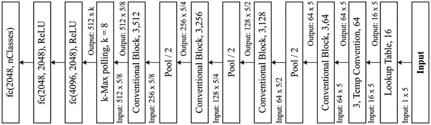
Figure 3: Architecture of VDCNN

They used another VDCNN for learning this parameter because the pair of biases and filters is critical in the reconstruction procedure. Smaller filter sizes, deeper layers, and extra filters could improve DL efficiency. The Media Source Extensions, as derived by Eq., is the cost function used at this stage (2). For minimizing the cost function, they utilized regular BP technique integrated by the arbitrary gradient decent technique for obtaining the optimum variables {W, B}.

L(W,B)=1n∑i=1n⁡‖F(Yi, Wi, Bi,)−Xi‖2 (2)

The variable pairs {W, B} was initiated with the help of Gaussian function using the distribution N(0, 0.001) . The filter upgrade task is displayed in Eq. (3), and the upgrade of bias is equivalent to filters.

Wi+1l=Wil+Δi+1 (3)

Δi+1=0.94+η∂L∂Wil

Whereas i and l denoted the iteration time and layer correspondingly, and four denotes the increase in the layer i. Since the variable pairs {W, B} attained in the training procedure could substantially enhance the reconstruction performance and speed, in this work, they selected this technique for studying the mapping relations among LR and HR frames and create an intermediate estimate frame.

3.2 Design of Curvelet Transform and SSIM

The intermediate video frames obtained from the LRHR relation mapping technique considered the relationship between the LR and HR picture blocks in a single frame, which does not use the whole spatio-temporal relation data between the nearby video frames. This data, on the other hand, could help to maintain the video's temporal dependability. Conventional fuzzy registration is based on the relationship between pixels in the neighbouring and target frames, which is typically defined as the weighted average of each adjacent pixel [19]. Whereas a single measurement would not be able to adapt well to the changing platform, in this work, they integrate the CLT and the SSIM for adjusting to local motion, rotation, and other minor changes in the dynamic scene.

SR films frequently contain objects with a variety of characteristics. This characteristic has edges that might be discontinuous or continuous. These edge-based discontinuities could be examined and tracked using CLT. In this method, separate objects with their associated edge data are labelled as curvelets, which can be seen via a multiscale directional transform. CLT is implemented in both continuous and discrete domains. The interpretations and turns of U polar wedge filter characterise the continuous CLT and is determined for 2−j scale in Eq. (6). Eq. (7) denotes the coarse curvelet filter where j ϵ N calculates the detail coefficient, for coarse and scale limit, the curvelet coefficient with translation xkj,l is displayed in Eq. (6).

∪j(r, Θ)=2−3j4V(2⌊j2⌋Θ2π) (4)

∪j(w)=2−j0W0(2−j0|w|) (5)

φj,k,l(x)=φj(Rl(x−xk(j,l))) (6)

φj0,k(x)=φj0(x−2−j0k)

The curvelet is determined in Eq. (7) for the function ′f′ that belong to R2 by curvelet coefficient as inner product of ‘f’.

c(j,l,k)=⟨f,φj,l,k⟩=∫R2⁡f(x)φj,l,k(x)dx¯ (7)

whereas, w: Cartesian form parameter, r, Θ: polar form parameters, r ≥ 0, Θϵ[0,2π) , j0: window function, j0 ≤ jϵ N, W: radial window function, V : angular window function through 2π period, R: Rotatel, φj,k,l(x): spatial mother curvelet function, x: spatial space parameter vector, l: rotational variable, lϵ N0, and k: translation variable, kϵ Z2.

Depending upon the orientation and scale, the curvelet coefficient is collected to different sub bands and curvelet coefficients are calculated for all the sub bands. Afterward calculating the curvelet coefficient, the normalized directional energy Ei (Ei the energy of ith subband) is calculated for all the curvelet subbands by L1 norm displayed in Eq. (9). The last curvelet feature vector is denoted by:

fCT=[E1 E2 E3 E4 E5 E6… Ens] (8)

Whereas ns denotes the overall amount of curvelet sub bands.

Ei=1m×n∑x=1m⁡∑y=1n⁡ci(x, y) (9)

Whereas Ei denotes the energy of ith subband coefficient and ci indicates the curvelet coefficient of sub band i with dimension m × n.

For SSIM, assume 2 areas placed in pixels (i, j) & (k, l), and noted as Rij & Rkl, correspondingly, they calculated their mean μ & standard deviation σ and covariance among these 2 regions as cov(i, j, k, l) Depending upon these predetermined values, they could attain the SSIM as displayed in Eq. (10), whereas e1 & e2 denotes constant.

SRSS(Rij,Rkl)=(2μ(k,l)μ(i,j)+e1)(2cov(k,l,i,j)+e2)(μ(k,l)2+μ(i,j)2+e1)(σ(k,l)2+σ(i,j)2+e2) (10)

For all the search regions centered in (k, l) is reconstructed frame, noted as Rkl, they traversed their nearby pixel points (i, j) in local window mark as R with predefined size and calculated the SSIM among 2 areas. Using a predetermined threshold, the area that is not equivalent to Rkl would be filtered out. Therefore, the CLT SCLT(Rij, Rkl) was considered as the core indicator and SSIM SRSS(Rij, Rkl) was used for fine tuning this similarity with a smaller weight λ, that would be fixed as 0.000 2 in last research. Mark the nearby areas that must be selected from an adjacent frame and single frame.

ω(k,l,i,j)=1C(k,l)SZFS(Rij, Rkl)(1−λSRSS (Rij, Rkl)) (11)

where (i, j) represents the searched pixels in a nonlocal search region, C(k, l) represents the normalized constant determined by Eq. (12), and the variable ϵ is utilized to control the weight decay rate.

C(k,l)=∑(i,j)∈Rsr(k,l)⁡e‖Zkl−Zij‖22ϵ2(1−λSRSS(Rij,Rkl)) (12)

Whereas Rsr(k, l) represents the searching region. Afterward calculating the similarity among the video frames, they can attain the weight of subregions based on Eq. (11), with appropriate regions that could be chosen. Later, this area has been merged iteratively for obtaining a frame closer to original. In order to pixel (k, l) that exists super-resolved, they would restructure it by the SR estimate energy function by:

x^(k,l)=arg min ‖x(k,l)−∑T=T1T2⁡∑(i,j)∈Rsr(k,l)⁡ω(k,l, i,j,T)x(i,j)‖22 (13)

Whereas x(k, l) represents the older energy value in pixel (k, l) and x^(k,l) denotes the target value. Now, they presented the variable T as frame amount of the traversed pixel (i, j) to represents the relation among distinct frames. [T1, T2] denotes the frame amount of range the searching image handled by the search amount N generally, it could be expressed as [T0 − N, T0 + N]. Afterward minimalizing this function, they can proceed with a closed form solution by:

x^(k,l)=∑(k,l)∈Ψ⁡∑T∈[T1T2]⁡∑(i,j)∈Rsr(k,l)⁡ω(k,l,i,j,T)x(i,j,T)∑(k,l)∈Ψ⁡∑T∈[T1T2]⁡∑(i,j)∈R1(kl)⁡ω(k,l,i,j,T) (14)

3.3 Model Representation in Digital Twins

Grieves established the Digital Twin model and notion because the conceptual module underpins Product Lifecycle Management [20]. Despite the fact that the phrase was not used previously, the main components of each Digital Twin have been defined: virtual space, physical space, and the data flow between them. The fundamental enablers of Digital Twins: Closed Captioning, Artificial Intelligence, Internet of Things (IoT), Big Data, and sensor technologies have grown at an astonishing rate. Currently, NASA defines a Digital Twin as a multiscale, Multiphysics, ultra-fidelity simulation, probabilistic that allows real-world reproduction of the state of a physical object in cyberspace based on real-world sensor and historical data. Tao et al. expanded the module and proposed that Digital Twin modelling must comprise the following elements: virtual modelling, physical modelling, data modelling, service modelling, and connection modelling.

Innovative technologies are paving the way for smart cities, in which every physical object would have communication capabilities and embedded computing, allowing them to detect the platform and interact with one another to provide services. Machine-to-Machine Communication/IoT is another term for intelligent interoperability and linkages [21]. A smart city must have a smart home, smart energy, smart manufacturing, and a smart transportation system. Data capture becomes comparably simple due to the availability and affordability of actuators and sensors. One of the challenging tasks is diagnosing and monitoring manufacturing machinery via the Internet. The merging of the virtual and physical worlds of manufacturing is a major issue in the field of Cyber-Physical Systems (CPS) that demands additional research.

The concept of a “digital twin” is the creation of a module of a physical asset for the purpose of forecasting maintenance. Using real-world sensory data, this method would usually be used to anticipate the forthcoming of relevant physical resources in the operation/environment. It might discover and monitor potential threats posed by its physical counterpart. It is divided into three sections: I virtual products in virtual space, (ii) physical items in actual space, and (iii) a combination of virtual and real products. As a result, evaluating and collecting a massive amount of manufacturing data in order to uncover the data and relationship becomes critical for smart manufacturing. General Electric has begun their digital transformation path, which is centred on Digital Twin, by building critical jet engine modules that forecast the business results associated to the residual life of these modules. In this study, a new video reconstruction technique for digital twins is devised, which aids in real-time performance.

The concept engaged in the extensive reference approach is to broaden and hand over the conceptual model while conveying the scientific fundamentals of video reconstruction standards to the aspect of digital twins. The proposed concept is focused on “twinning” between the physical and virtual spheres. As a result, a digital twin model may be created using an abstract technique that includes all of the traits and completely explains the physical twin at a conceptual level. Thought simulations are performed based on the abstract model, allowing for the capture and understanding of the physical twin at an abstract level.

3.4 Steps Involved in Proposed Model

Based on the aforementioned procedures, the projected method is given below. Now, this technique is separated into 2 phases: reconstruction and training processes.

Input LR video sequence {Xt,t}t=1T , SR factor s, HR training data THR, LR trained data TLR, the amount of NN layers L, the filter size f, and the filter amount n, for all the layers. The nearby searching frame N, weight control variable ϵ , and the round number K.

Outcome HR video sequence {Yt,t}t=1T.

Training procedure Input the training sets THR & TLR into the VDCNN and utilize BP for obtaining an optimum {W,B} variable pairs.

SR Reconstruction Procedure

Step 1 Utilize the bi-cubic method for obtaining an early estimation of LR video sequence, mark as {Xt′,t}t=1T.

Step 2 For {Xt′,t}t=1T, plug the variable pairs {W,B} attained from the training procedure for getting the in-between outcomes {Yt′,t}t=1T by VDCNN.

Step 3 Enlarge the edge of frame yt′ and its nearby frames, and note the enlarged frames as {ysE}t−Nt+N.

Step 4 Traverse the reconstructed frame yt′ and attain the reconstructed block Rkl.

Step 5 Traverse the nearby region of Rkl in {ysE}t−Nt+N and attain the blocks that should be merged, mark this block as {Rij}(i,j)∈Rsr(k,l).

Step 6 Calculate the SSIM among Rkl & Rij and evaluate when Rij is equivalent to the reconstructed block. When this region is not equivalent as recommended, proceed to Step-8 for getting the subsequent block, otherwise note the similar regions as Ri^j^.

Step 7 For Rkl, upgrade its weight.

Step 8 When there exist other blocks in {Rij}(i,j)∈Rsr(k,l), proceed to Step 5 for getting the subsequent block, otherwise, proceed to Step 10.

Step 9 Merge the group of equivalent areas Ri^j^ to attain the target block Rkl∗.

Step 10 When other blocks are existed in the reconstructed frames, proceed to Step 4 for getting the subsequent blocks, otherwise the target frame {Yt,t}t=1T is attained.

Step 11 Update repetitively: when the round amount k is lesser compared to present maximal K, continue to Steps 3 & 4; or else, stop the process.

4  Performance Validation

The proposed VDCNN-SS technique's SR video reconstruction performance is examined in terms of several factors. Tab. 1 compares the Peak signal-to-noise ratio (PSNR) and SSIM of the VDCNN-SS technique to other known algorithms on four datasets.

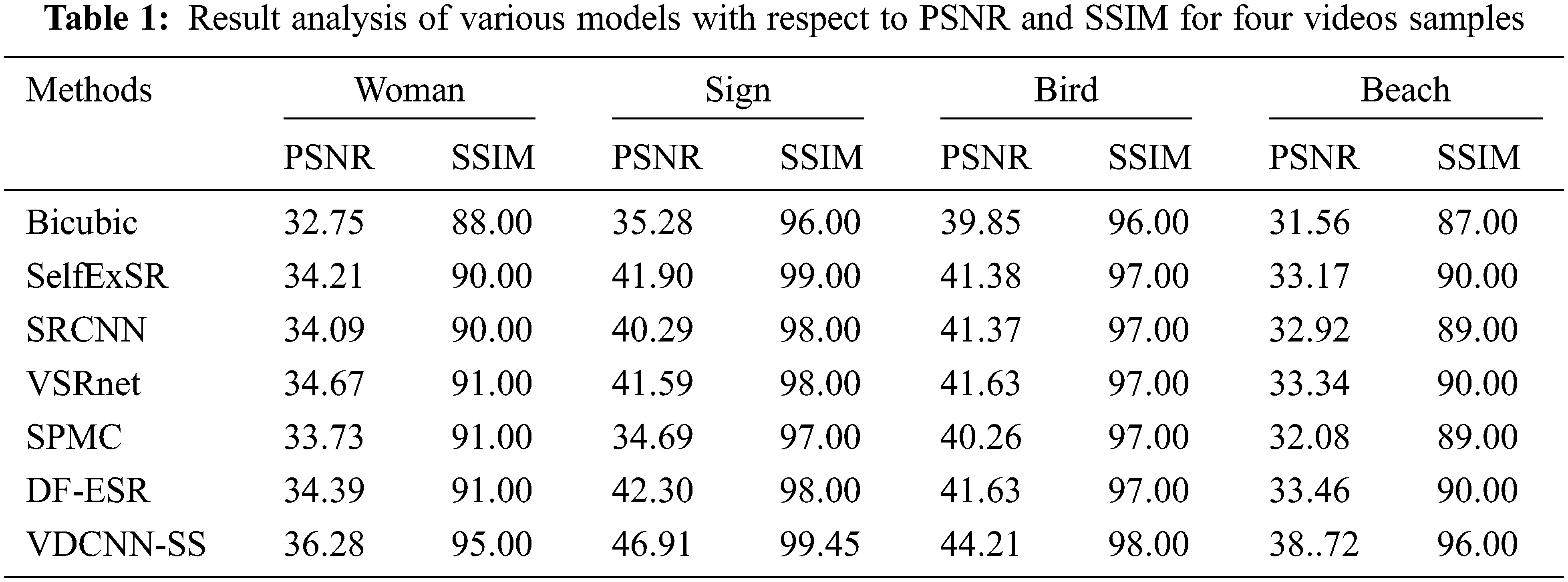
Fig. 4 compares the performance of the VDCNN-SS technique to other strategies in terms of PSNR on four test movies. The figure shows that the VDCNN-SS technique achieved an effective result by providing maximum PSNR values on the used videos. For example, on the applied lady video, the VDCNN-SS technique achieved a greater PSNR of 36.28 dB, but the Bicubic, SelfExSR, SRCNN, VSRnet, sub-pixel motion compensation (SPMC), and Deep Fusion- Enhanced Super-Resolution (DF-ESR) procedures achieved lower PSNRs of 32.75, 34.21, 34.09, 34.67, 33.73, and 34.39 dB, respectively. Furthermore, on the used Sign video, the VDCNN-SS technique produced a superior PSNR of 46.91 dB, whereas the Bicubic, SelfExSR, SRCNN, VSRnet, SPMC, and DF-ESR methods achieved a minimum PSNR of 35.28, 41.90, 40.29, 41.59, 34.69, and 42.30 dB, respectively. Finally, on the used bird video, the VDCNN-SS technique obtained a maximum PSNR of 44.21 dB, whereas the Bicubic, SelfExSR, SRCNN, VSRnet, SPMC, and DF-ESR methods obtained lower PSNRs of 39.85, 41.38, 41.37, 41.63, 40.26, and 41.63 dB, respectively. Furthermore, on the applied beach video, the VDCNN-SS approach achieved a greater PSNR of 38.72 dB, whereas the Bicubic, SelfExSR, SRCNN, VSRnet, SPMC, and DF-ESR techniques achieved a minimal PSNR of 31.56, 33.17, 32.92, 33.34, 32.08, and 33.46 dB, respectively.

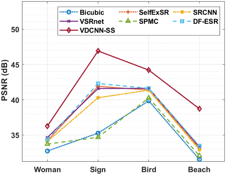
Figure 4: Result analysis of VDCNN-SS model in terms of PSNR

Fig. 5 compares the performance of the VDCNN-SS method to other approaches in terms of SSIM on four test movies. According to the graph, the VDCNN-SS method achieved an effective outcome by providing maximum SSIM values on the applied videos. For example, on the applied lady video, the VDCNN-SS method obtained an improved SSIM of 95, whilst the Bicubic, SelfExSR, SRCNN, VSRnet, SPMC, and DF-ESR approaches obtained a minimal SSIM of 88, 90, 90, 91, 91, and 91, respectively. Following that, on the applied Sign video, the VDCNN-SS approach produced a higher SSIM of 99.45, but the Bicubic, SelfExSR, SRCNN, VSRnet, SPMC, and DF-ESR strategies obtained a lower SSIM of 96, 99, 98, 97, and 98, respectively. Furthermore, on the applied bird video, the VDCNN-SS methodology produced a superior SSIM of 98, whereas the Bicubic, SelfExSR, SRCNN, VSRnet, SPMC, and DF-ESR methods obtained a minimal SSIM of 96, 97, 97, 97, and 97, respectively. Finally, on the applied beach video, the VDCNN-SS methodology obtained a superior SSIM of 96, whilst the Bicubic, SelfExSR, SRCNN, VSRnet, SPMC, and DF-ESR algorithms obtained a minimum SSIM of 87, 90, 89, 90, 89, and 90, respectively.

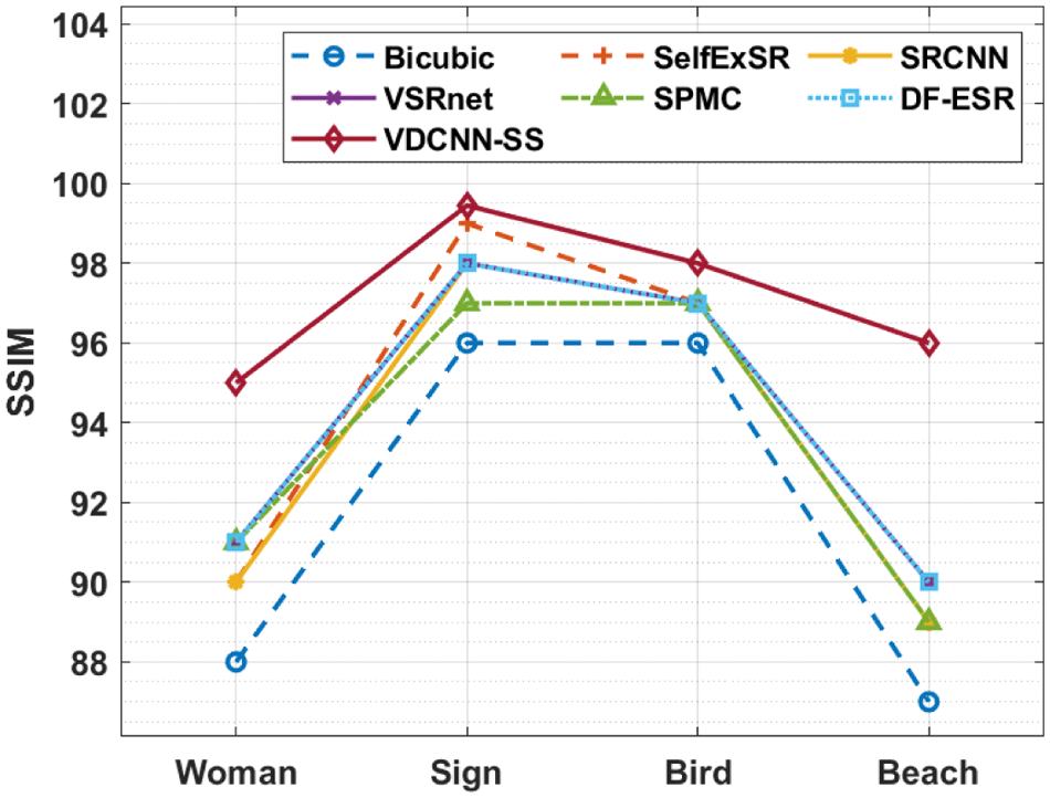
Figure 5: Result analysis of VDCNN-SS model in terms of SSIM

A series of simulations are run on a benchmark video dataset to further ensure the increased performance of the proposed technique. Fig. 6 depicts an example set of video frames from the used David dataset.

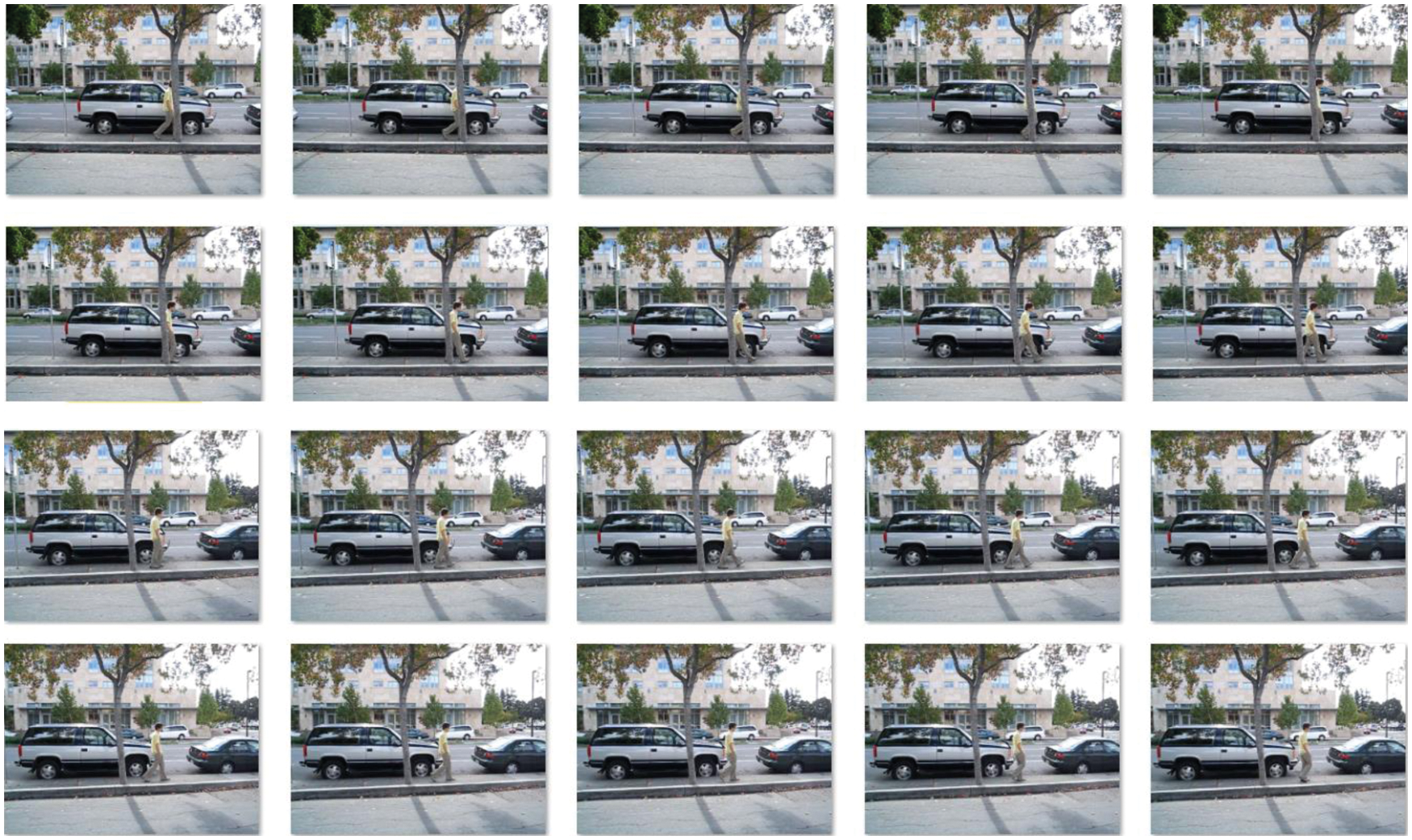
Figure 6: Sample images (David dataset)

Tab. 2 and Fig. 7 show a detailed PSNR comparison of the VDCNN-SS technique with existing techniques over a range of frame counts. The collected findings show that the VDCNN-SS technique achieved superior performance with the highest PSNR value. For example, under 10 frames, the VDCNN-SS technique yielded a better result with a PSNR of 35.98 dB, but the SPMC and DF-ESR procedures yielded lower results with PSNRs of 32.23 and 33.66 dB, respectively. Furthermore, under 30 frames, the VDCNN-SS method surpassed increased results with a PSNR of 35.12 dB, whilst the SPMC and DF-ESR methods fared poorly with PSNRs of 30.50 and 32.71 dB, respectively. Similarly, under 50 frames, the VDCNN-SS approach achieves the best results with a PSNR of 40.14 dB, while the SPMC and DF-ESR procedures achieve poorer results with PSNRs of 36.40 and 38.99 dB, respectively.

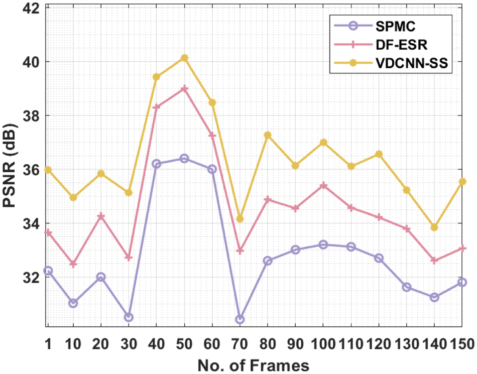
Figure 7: PNSR analysis of VDCNN-SS model on david dataset

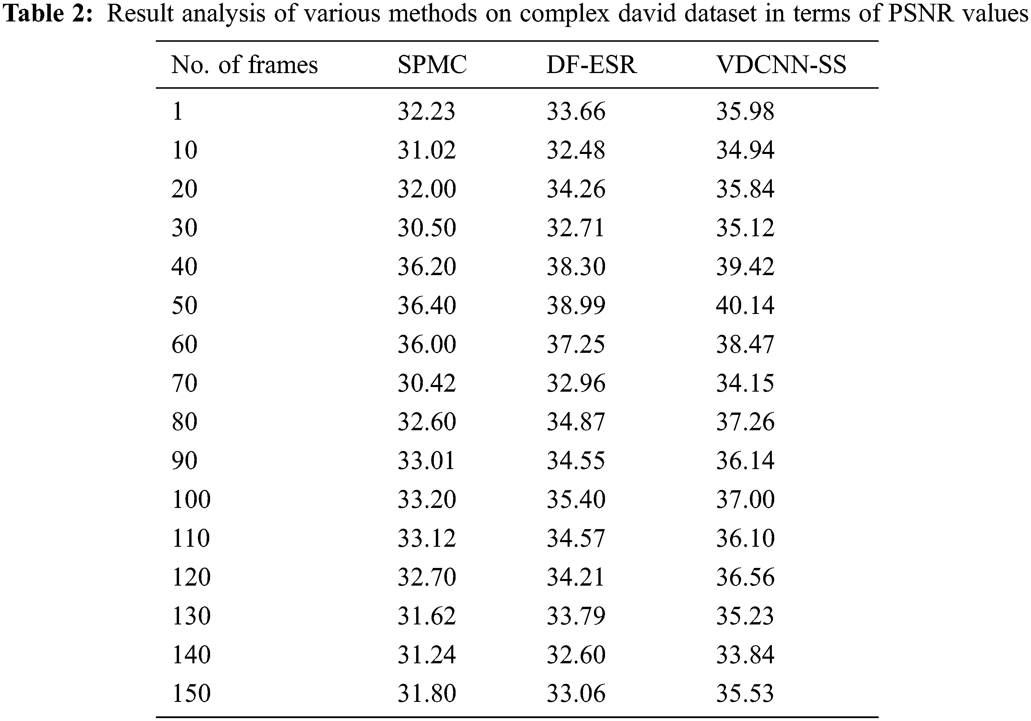
Simultaneously, under 70 frames, the VDCNN-SS methodology performed better with a PSNR of 34.15 dB, while the SPMC and DF-ESR methods fared worse with PSNRs of 30.42 and 32.96 dB, respectively. Concurrently, under 100 frames, the VDCNN-SS approach yielded a better result with a PSNR of 37 dB, whilst the SPMC and DF-ESR algorithms yielded the worst results with PSNRs of 33.20 and 35.40 dB, respectively. Under 130 frames, the VDCNN-SS method yielded a greater result with a PSNR of 35.23 dB, but the SPMC and DF-ESR procedures yielded lower results with PSNRs of 31.62 and 33.79 dB, respectively. Finally, within 150 frames, the VDCNN-SS technique achieves the best results with a PSNR of 35.53 dB, while the SPMC and DF-ESR algorithms achieve the worst results with PSNRs of 31.80 and 33.06 dB, respectively.

A series of simulations on benchmark video datasets are performed to further ensure the improved performance of the current technique. Fig. 8 depicts a sample set of video frames from the applied girl dataset [22].

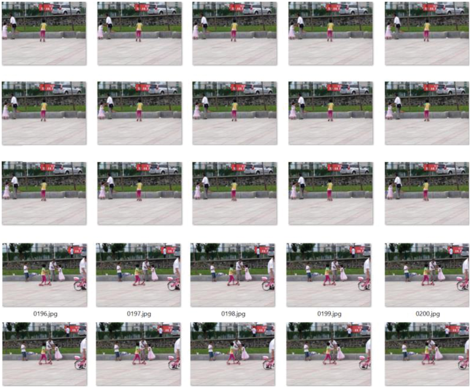
Figure 8: Sample images (Girl dataset)

Tab. 3 and Fig. 9 show a complete PSNR analysis of the VDCNN-SS method with existing techniques over a range of frame counts. The obtained results show that the VDCNN-SS approach achieved improved performance with the highest possible PSNR value. Under 100 frames, the VDCNN-SS method produced a better result with a PSNR of 42.76 dB, but the SPMC and DF-ESR methods produced a lower result with PSNRs of 36.13 and 39.27 dB, respectively. Also, under 300 frames, the VDCNN-SS technique performed better with a PSNR of 43.73 dB, but the SPMC and DF-ESR algorithms performed worse with PSNRs of 37.12 and 40.62 dB, respectively. Similarly, under 500 frames, the VDCNN-SS method yielded a higher result with a PSNR of 38.64 dB, but the SPMC and DF-ESR procedures yielded lower results with PSNRs of 34.97 and 37.33 dB, respectively.

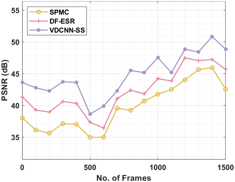
Figure 9: PNSR analysis of VDCNN-SS model on girl dataset

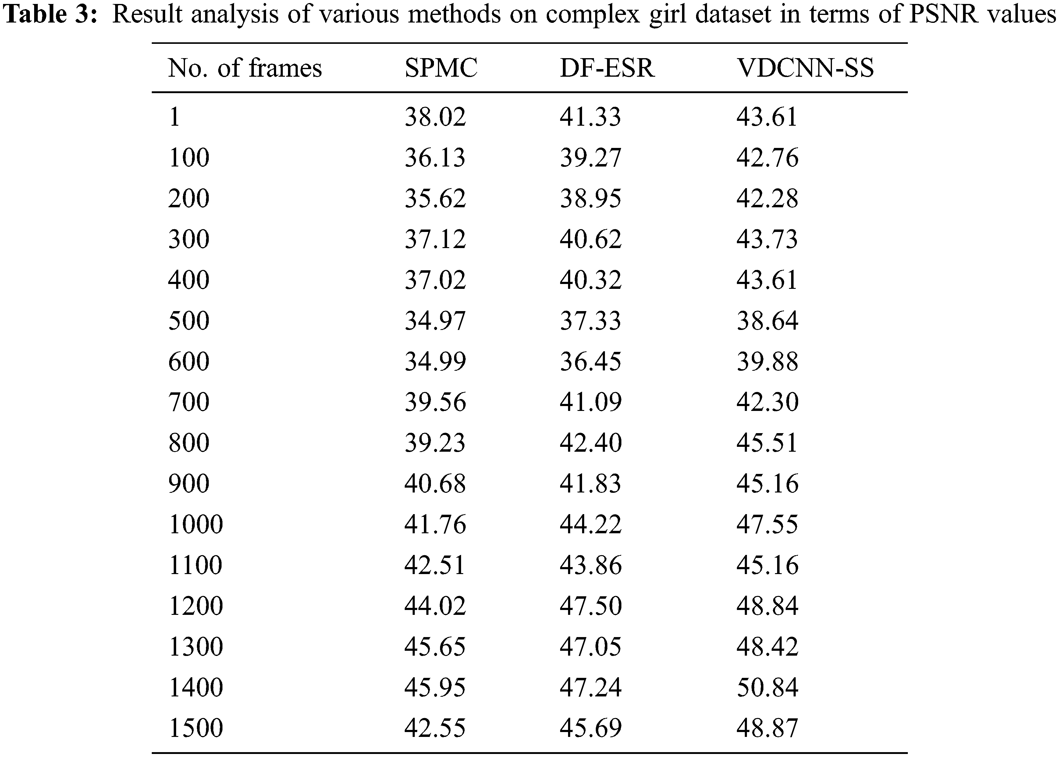
At the same time, under 700 frames, the VDCNN-SS strategy performed better with a PSNR of 42.30 dB, whilst the SPMC and DF-ESR strategies performed worse with PSNRs of 39.56 and 41.09 dB, respectively. Simultaneously, under 1000 frames, the VDCNN-SS approach yielded a better result with a PSNR of 47.55 dB, whilst the SPMC and DF-ESR procedures yielded lower results with PSNRs of 41.76 and 44.22 dB, respectively. Following that, under 1300 frames, the VDCNN-SS technique performed better with a PSNR of 48.42 dB, whilst the SPMC and DF-ESR approaches performed worse with PSNRs of 45.65 and 47.05 dB, respectively. Finally, under 1500 frames, the VDCNN-SS method fared better with a PSNR of 48.87 dB, while the SPMC and DF-ESR methods performed worse with PSNRs of 42.55 and 45.69 dB, respectively.

5  Conclusion

This research provided a novel VDCNN-SS technique for successful SR video reconstruction. The VDCNN-SS technique primarily employs the VDCNN model to acquire the reconstruction variables among the LR and HR picture blocks that increase the SR speed. Additionally, the use of CLT and SSIM occurs. The intermediate video frames obtained from the LRHR relation mapping technique considered the relationship between the LR and HR picture blocks in a single frame, which does not use the whole spatio-temporal relation data between the nearby video frames. A comprehensive simulation analysis is performed to examine the improved SR video reconstruction performance of the VDCNN-SS technique, and the findings are analysed in terms of several evaluation factors. The testing results demonstrated the superiority of the VDCNN-SS technique over the more modern techniques. The pretrained rebuilt coefficient can be used to speed up the SR video reconstruction process in the future. Furthermore, the reconstruction results can be improved by employing the optimization technique using SS.

Funding Statement: The authors received no specific funding for this study.

Conflicts of Interest: The authors declared that they have no conflicts of interest to report regarding the present study.

References

 1.  P. V. Rajaraman, “Intelligent deep learning based bidirectional long short term memory model for automated reply of e-mail client prototype,” Pattern Recognition Letters, vol. 152, no. 1, pp. 340–347, 2021. [Google Scholar]

 2.  R. Chithambaramani and P. Mohan, “Addressing semantics standards for cloud portability and interoperability in multi cloud environment,” Symmetry, vol. 13, no. 2, pp. 1–18, 2021. [Google Scholar]

 3.  D. Paulraj, “An automated learning model of conventional neural network based sentiment analysis on twitter data,” Journal of Computational and Theoretical Nano Science, vol. 17, no. 5, pp. 2230–2236, 2020. [Google Scholar]

 4.  D. N. Doulamis, D. Anastasios, K. Panagiotis and M. V. Emmanouel, “Event detection in twitter microblogging,” IEEE Transactions on Cybernetics, vol. 46, no. 12, pp. 2810–2824, 2015. [Google Scholar]

 5.  Y. Li, Z. Zhen, P. You, Y. Hongzhi and X. Quanqing, “Matching user accounts based on user generated content across social networks,” Future Generation Computer Systems, vol. 83, pp. 104–115, 2018. [Google Scholar]

 6.  R. Annamalai, “Social media network owings to disruptions for effective learning,” Procedia Computer Science, vol. 172, no. 5, pp. 145–151, 2020. [Google Scholar]

 7.  K. Makantasis, D. Anastasios, D. Nikolaos and I. Marinos, “In the wild image retrieval and clustering for 3D cultural heritage landmarks reconstruction,” Multimedia Tools and Applications, vol. 75, no. 7, pp. 3593–3629, 2016. [Google Scholar]

 8.  S. Neelakandan and M. Dineshkumar, “Decentralized access control of data in cloud services using key policy attribute based encryption,” International Journal for Scientific Research & Development, vol. 3, no. 2, pp. 2016–2020, 2015. [Google Scholar]

 9.  D. Venu, A. V. R. Mayuri, G. L. N. Murthy, N. Arulkumar and S. Nilesh, “An efficient low complexity compression based optimal homomorphic encryption for secure fiber optic communication,” Optik, vol. 252, no. 1, pp.168545, 2022. [Google Scholar]

10. A. L. Mur, P. Françoise and D. Nicolas, “Recurrent neural networks for compressive video reconstruction,” in 2020 IEEE 17th Int. Symp. on Biomedical Imaging (ISBI), Iowa City, IA, USA, pp. 1651–1654, 2020. [Google Scholar]

11. H. Yao, D. Feng, Z. Shiliang, Z. Yongdong, T. Qi et al., “Dr2-net: Deep residual reconstruction network for image compressive sensing,” Neurocomputing, vol. 359, pp. 483–493, 2019. [Google Scholar]

12. B. P. Sankaralingam, U. Sarangapani and R. Thangavelu, “An efficient agro-meteorological model for evaluating and forecasting weather conditions using support vector machine,” in Proc. of First Int. Conf. on Information and Communication Technology for Intelligent Systems, India, pp. 65–75, 2016. [Google Scholar]

13. M. Sundaram, S. Satpathy and S. Das, “An efficient technique for cloud storage using secured de-duplication algorithm,” Journal of Intelligent & Fuzzy Systems, vol. 42, no. 2, pp. 2969–2980, 2021. [Google Scholar]

14. C. F. Higham, M. S. Roderick, J. P. Miles and P. E. Matthew, “Deep learning for real-time single-pixel video,” Scientific Reports, vol. 8, no. 1, pp. 1–9, 2018. [Google Scholar]

15. M. Prakash and T. Ravichandran, “An efficient resource selection and binding model for job scheduling in grid,” European Journal of Scientific Research, vol. 81, no. 4, pp. 450–458, 2012. [Google Scholar]

16. C. Kong, C. Jun-Tao, L. Yun-Fei and C. Ruo-Yu, “Deep learning methods for super-resolution reconstruction of temperature fields in a supersonic combustor,” AIP Advances, vol. 10, no. 11, pp. 115021, 2020. [Google Scholar]

17. A. M. Judith and S. B. Priya, “Multiset task related component analysis (M-TRCA) for SSVEP frequency recognition in BCI,” Journal of Ambient Intelligence and Humanized Computing, vol. 12, no. 5, pp. 5117–5126, 2021. [Google Scholar]

18. P. Asha, L. Natrayan, B. T. Geetha, J. Rene Beulah, R. Sumathy et al., “IoT enabled environmental toxicology for air pollution monitoring using AI techniques,” Environmental Research, vol. 205, no. 1, pp. 1–12, 2022. [Google Scholar]

19. C. Ramalingam, “An efficient applications cloud interoperability framework using i-anfis,” Symmetry, vol. 13, no. 2, pp. 1–12, 2021. [Google Scholar]

20. P. Mohan and R. Thangavel, “Resource selection in grid environment based on trust evaluation using feedback and performance,” American Journal of Applied Sciences, vol. 10, no. 8, pp. 924–930, 2013. [Google Scholar]

21. S. Neelakandan, A. Arun, R. R. Bhukya, B. M. Hardas, T. Ch et al., “An automated word embedding with parameter tuned model for web crawling,” Intelligent Automation & Soft Computing, vol. 32, no. 3, pp. 1617–1632, 2022. [Google Scholar]

22. D. Comaniciu, V. Ramesh and P. Meer. Kernel-Based Object Tracking. PAMI, vol. 25, no. 5, pp. 564–577, 2003, http://cvlab.hanyang.ac.kr/tracker_benchmark/datasets.html. [Google Scholar]

This work is licensed under a Creative Commons Attribution 4.0 International License, which permits unrestricted use, distribution, and reproduction in any medium, provided the original work is properly cited.