DOI:10.32604/iasc.2022.025695
| Intelligent Automation & Soft Computing DOI:10.32604/iasc.2022.025695 | |
| Article |
4D Facial Expression Recognition Using Geometric Landmark-based Axes-angle Feature Extraction
Computer Engineering Department, Cyprus International University, Nicosia, North Cyprus, Mersin 10, 099010, Turkey
*Corresponding Author: Henry Ugochukwu Ukwu. Email: 20169216@student.ciu.edu.tr
Received: 01 December 2021; Accepted: 19 January 2022
Abstract: The primary goal of this paper is to describe a proposed framework for identifying human face expressions. A methodology has been proposed and developed to identify facial emotions using an axes-angular feature extracted from facial landmarks for 4D dynamic facial expression video data. The 4D facial expression recognition (FER) problem is modeled as an unbalanced problem using the full video sequence. The proposed dataset includes landmarks that are positioned to be fiducial features: around the brows, eyes, nose, cheeks, and lips. Following the initial facial landmark preprocessing, feature extraction is carried out. Input feature vectors from gamma axes and magnitudes in three-dimensional Euclidean space are constructed. This paper develops a new feature vector by concatenating the angle and magnitude features and compares them to a model created independently using angle features. In all three models, several filter-based feature selection techniques are used to estimate feature importance. The framework employs a multi-class support vector machine (SVM) on MATLAB, and the true positive rate (TPR) and average recognition rates (ARR) are used as performance metrics. In terms of average classification accuracy, the final results are compared to conventional state-of-the-art approaches. The results revealed a highly informative combined feature, demonstrating the efficiency of the proposed landmark-based strategy to classify facial expressions.
Keywords: Computer vision; facial expression recognition (FER); 4D dynamic facial expression; image processing; axes-angle feature
In the field of emotion recognition, heterogeneous derived features for image pairs are estimated, i.e., variations of feature points or texture changes. The principle or reasoning behind this work is that decoding facial expressions can be an unobtrusive way to investigate the basic emotional state of a person [1,2]. With this in mind, the psychological network has compiled comprehensive background literature in order to identify models that can accurately and completely depict facial emotions. In the nineteenth century, Charles Darwin pioneered the study of facial expressions. In 1872, Darwin identified the broad principles of facial expression in humans and animals, as well as the means of expression [3]. Face expressions were also classified by Darwin into groups. The basic categories are anxiety, joy, anger, surprise, disgust, sulkiness, and shyness, each of which has several subcategories. Darwin also outlined the facial deformities that occur with each type of expression. The discrete classification proposed in holocultural research led by Ekman et al. [4,5], which presents six essential or basic expressions that are universally recognized: happy, anger, sadness, fear, disgust, and surprise, is one of the most widely used models. The Facial Action Coding System (FACS) was proposed by the pioneers of this study in the 1970s to encode facial expressions with facial movements known as action units (AUs) [6–8].
The use of facial expression analysis and synthesis in multimedia systems (Moving Pictures Expert Group 4, MPEG-4 standard) became extremely widespread in the late 1990s, thanks to significant advancements recorded in the fields of computer graphics and imaging. The major goal was to animate or make the facial movements. In 1999, the MPEG4 standard included a face model with 83 characteristic points known as Facial Definition Parameters (FDPs) [9], which describe a face in its neutral condition. The MPEG-4 standard additionally included 68 Facial Animation Parameters (FAPs) for animating the face with feature point motions. FAPs can be used to animate and mix facial expressions, as well as to represent facial expressions in a traditional face model. Furthermore, FAPs produced from MPEG-4 are commonly used for facial expression synthesis in most research laboratories [9–11]. In this paper, consideration is given to features computed based on 83 detected facial landmarks on each facial mesh or frame, analyzing the angles of the features and the distances between feature landmark points. It is pertinent to draw attention to similar work related to previous or current breakthroughs in three-dimension 3D and four-dimension 4D facial expression recognition systems.
Facial landmarks FL can be described as highlights or corner points that are visible on the face, such as the area around the corners of the eyes, mouth corners, the nose, the eyebrow, the cheeks, and the jaw, as shown in Fig. 2 below [12]. In a facial expression recognition FER system, the angle of this FL around the 3D space and the point-to-center or point-to-point correspondences of these facial landmarks can be used to create a feature vector of a human face in a FER system. This is facilitated by the location or coordinates of all the landmarks around the facial area in the event of carrying out different actions or expressions. FER research has evolved greatly based on this fundamental insight, and an intriguing new FER approach has been proposed. They can be roughly categorized as geometric landmarks FER from dynamic 4D (or 3D+time) facial scans [13], and the multi-class FER problem is modeled as an unbalanced (full sequence) dataset.
Thus, the general implementation can be categorized into several stages: facial landmark preprocessing stage, visualization and analysis of data, feature extraction, feature selection, and classification of emotions. An appropriate 4D dataset, BU4DFE, with public access, essentially consisting of humans displaying labeled emotions of varying intensities in the images, will be used as test and training data [14,15]. Several conventional methods have explored feature extraction by finding distances or magnitudes. Hence the need to explore a more robust technique that utilizes angles as predictors and is rotation invariant. The proposed feature extraction method takes advantage of the 3D landmark data with respect to the three-dimensional axes XY, XZ, and YZ. Existing methods attempt to compute these predictors by finding the angle between feature points. In this paper, we consider the frontal face view, and as such, the XY plane is used in this work as the rotation or view is around the Z-axis. The proposed geometric-based facial features are given as input to a feature selection algorithm in the third phase, which selects ideal feature vectors based on feature relevance or ranks generated from feature weights. The primary motivation behind the implementation of feature selection is to reduce or eliminate overfitting. Reducing the dimension of our proposed dataset not only reduces the overfitting of the model, but also ensures certain amplified performance, rapid training, less cost, less storage space required for the data, and the removal of noise and irrelevant predictors. Implementing the procedure with and without feature selection demonstrates the influence of feature selection (without-Fs).
In the final step, the selected vectors are then sent to a classification network that has been trained to classify which emotion is conveyed. The terms “features” and “predictors” are used interchangeably in this paper.
In light of the above discussion, our 2-fold contributions to this work are as follows: We present an extension to geometric-based 4D FER that provides a simple yet efficient method to handle 3D and 4D data limitation problems. Despite the existing limitations of not being translation and/or rotation invariant, magnitude feature vectors have been explored by researchers for several years. As a result, a more robust feature space that is invariant to rotations containing angle predictors in whole or in part is essential. Hence the three methods: magnitude, angle, and combined (angle + magnitude). We introduce axes-angular over three axes to extract angle landmark features known as gamma angle predictors. We compute magnitudes for all feature points to the origin. The axes angles formed from the feature points to the origin are concatenated with the magnitudes to create a rich feature vector that outperforms state-of-the-art performance at reduced computational speed. Although the focus is on comparing recognition accuracy rather than execution time, the reduced complexity of the model in this paper is represented by capturing the feature space and feature count. Our contribution and novelty could be highlighted by the fact that, from the given 3D landmark data, we harnessed its landmark orientation relative to the origin (0, 0, 0), in contrast to some recent works [16–18] that attempted to compute the angles between the feature points. However, to the best of our knowledge, we can claim that it is the first time that an axes-angular feature of 3D landmarks has been used in a 4D FER. This is indeed the novelty of our work and has not been reported before. Also, for the first time, several filter-based feature selection techniques (Neighborhood component feature selection NCFS, RELIEF, and minimum redundancy maximum relevance FMRMR, etc.) are applied to 4D FER to achieve a reduced feature space. The rest of the paper is organized as follows: Section 2 presents the related work in facial emotional expression, and Section 3 explains our proposed 4D FER method. In Section 4, we show and analyze our experimental results to validate the effectiveness of the proposed method. Finally, the paper's conclusion is recorded in Section 5.
Different authors have brought forward different approaches for facial expression recognition systems (FER). Some of these methods have been for facial feature analysis, others for semantic or hybrid methods, etc. To understand the basic ideas of face geometry, a number of methods are reported in [18] that depend only on static 3D data, i.e., mostly on apex frames. Due to its importance in improving performance, 4D FER has received a lot of attention in the last ten years. This is because 4D data provide complimentary spatial-temporal patterns that help deep models better interpret and predict facial expressions [19]. Interesting ways to learn facial muscle patterns over a period of time were explored by [20,21] using the famous Hidden Markov Model (HMM). Recently, the mode of the capture of 3D scans has changed such that, with skill and systematic application of robust techniques, it has become feasible for the characteristic features around the facial area of interest to be extracted.
There are cases where the advantages of feature-based and model-based methods have been considered to develop a novel method through the use of a muscular movement model [22]. The paper elaborates on the developing geometric features (e.g., coordinate index, normal index, and shape index) that are developed from 11 muscle regions to describe the facial shape characteristics. Then, a genetic algorithm learns the weights of the several sections, and SVM and HMM classifiers are used for expression prediction in 3D and 4D FER, respectively. The reference [23] proposed an AU recognition system that manually labels eight AUs in the BU-4DFE database, but their annotations are private. The author in [24] used BU-3DFE with 83 people and proposed 3D geometrical facial feature point positions + SVM. Entropy is utilized to extricate the most discriminative predictors [25]. The reference [26] used BU-3DFE and worked on the 3D flow of facial points+SVM+6E Neutral 3D facial model for each subject. The author in [27] used BU4DFE and Grassmannian manifold + SVM without any computationally expensive preprocessing steps or user intervention. Generally, dynamic systems operate on 3D image sequences for facial expression analysis. In much of the research, 3D-based FER showed better accuracy than two-dimensional FER. Three and four-dimensional FER also have certain problems bordering around the high computational cost of high resolution and frame rate, which also have data involved [28].
In the early 2000s, we began to see the results of combining 2D and 3D data. These algorithms fuse varying features like landmark coordinates, texture data, facial shape information, and facial curvature [29]. This kind of multimodal 2D+3D is a popular approach for facial expression recognition, widely used in [30,31]. Although we have seen good performance using 3D data [32], which supersedes that of 2D data, the fusion of two modalities provides even higher detection rates [33]. Automatic deep networks have been promising in the processing of dynamic FER [34]. Reference [35–37] are all studies conducted using deep learning-based methods, and they generated the deep representation of the 3D face by putting the geometry map, normal maps, normalized curvature map, and texture map into a pre-trained convolutional neural network CNN. Facial geometric attributes are then classified using SVM, and other classifiers to achieve substantial facial expression prediction. The authors in [14] proposed a novel augmentation technique that serves to combat the data limitation problem for deep learning (long short-term memory, LSTM) and [38–40], also providing clarity on the subject.
Using 3D facial landmarks, we perform facial expression recognition on the facial expression database by analyzing the performance using metrics described in subsection 2.7, and comparing our results to the other state-of-the-art conventional Euclidean distance-based methods.
2.1 Facial Expression Database
To conduct our experiments, a state-of-the-art 4D facial database was used. The database is the BU-4DFE [15], which consists of 101 subjects displaying 6 prototypic facial expressions (anger, happiness, fear, disgust, sadness, and surprise). There are fifty-eight (58) females and forty-three (43) male participants, ranging in age from 18 to 45, with a diversity of ethnic and racial ancestries. The length of the video sequence for each expression is not equal, but they are all around 100 seconds long. It is possible to visualize the key-frames from each sequence based on varying intensity levels (neutral, onset, apex, offset). The resolution of each 3D model is around 35,000 vertices, and its geometric landmark positions could be visualized (see Fig. 1). This involves a multi-class classification setting with 6 classes. The distribution of the classes is fairly skewed. However, because all of the classes are roughly equal, the resulting data is fairly unbalanced.

Figure 1: Shows feature point angles (x, y, z), for the BU4DFE dataset. (Source. [15])
Based on the model detailed in section 2, 83 facial landmarks are detected in the datasets [41]. From these landmarks, an eighty-three-dimension vector is constructed to represent each face and expression (eighty-three 3D landmarks (x, y, z). The initial model vector of about 105,000 dimensions (obtained from 35,000 3D vertices of the original model) is reduced to an 83-dimension vector by employing these face feature vectors, while still preserving a high degree of accuracy for expression detection. We show that using this experimental design results in the accurate recognition of facial expressions.
We adopt a novel approach in this paper by investigating the information present in feature point angles to the origin on three planes or axes in 3D space that are valuable or sufficient for effective emotion recognition. Fig. 2 is a block diagram depicting the proposed network’s structure. The 4D FER is a set of three experiments, each with at least three steps. The video processing, feature extraction, and feature selection are using Neighborhood Component Feature Selection NCFS, RELIEF and minimum redundancy maximum relevance FMRMR approaches. The experiments were performed without a feature selection block to validate the need for a reduced feature set. Finally, results obtained from the classification stage of all the experiments may be compared.

Figure 2: Structure of the proposed network
The geometric details for each frame in the video sequence for all facial expressions are quantitatively analyzed. This strategy is positioned to raise the computational complexity for generic dynamic expression classification by only using landmark features for the complete video frame sequence. For geometric landmark processing, min-max normalization of combined features is performed after the concatenation of the extracted axes-angle and magnitude features. Here the landmarks are organized in matrix form, with each row depicting observations and the columns depicting feature points. Each subject in the dataset has folders containing video sequences for all six-expression classes. In order to extract features, the proposed algorithm traverses each sequence for all 101 subjects and organizes them into rows. The feature matrix for full sequence processing is of size m*n, where m is 60,402 and n is 83. All of the observations are used to process the labels; their dimension is k*s, where k equals 60,402 and s equals 1.
Angle deformations alone are scale and rotation invariant; therefore, they don't need to be normalized. The face landmarks in 3D space are depicted in Fig. 3. Understanding the equation of axes angular extraction represented in Eqs. (1) and (2) is the first step in implementing feature extraction.

Figure 3: A representation of a three-dimensional with Z pointing towards the observer (Frontal view) face in BU-4DFE
The line segment (also known as a vector) that connects an origin Pc (0, 0, 0) to every feature point P (x, y, z) in space can be used to label each feature point P (x, y, z) in space. The angles between the lines and the axes could be calculated with respect to the different axes in the 3D Euclidean space.
Where Fp represents the feature point and Q represents the number of feature points, Xc is the origin or center of three-dimensional (3D) space ℝ3. The parameters Xp, Yp, and Zp represent landmark coordinates for geometric landmark points.
After extracting angle features alone using Eq. (1), we construct a combined feature vector (Angle + Magnitude) and normalize the vector in this paper since angles are measured in radians and magnitudes/distances are a measure of coordinates. The following are the 166 features used: distance from the origin to the feature point (83), and angles of the feature point to the origin (83). The angles of all points to the origin with respect to the XY axes measured in radians are derived by keeping the Z components constant. It is mathematically expressed in Eqs. (1) and (2) as thus:
where p = 1, 2, 3… Q.
2.3.3 Standardization / Z-Score Normalization
This is performed so that the features are rescaled to inherit the properties of a standard normal distribution with mean μ = 0 and standard deviation from the mean σ = 1. Standardizing the features or applying the min-max normalization technique makes the data scale to a fixed range, usually 0 to 1. It is expressed in Eqs. (3) and (4) as follows:
Considering 60,402 samples and the number of experiments, it might be desirable to lower the number of predictors for faster computations using filter feature selection approaches since they do not need training the models, a quality that makes it substantially faster than wrapper methods [42]. The NCFS, RELIEF, and FMRMR algorithms [43] are used in this paper. However, we focus on the performance or recognition accuracy rather than report the time complexities. The experiment takes the threshold point for feature ranking as the mean weights or scores during the subset feature selection process.
Neighborhood Component Analysis (NCA) is a supervised distribution strategy that maximizes deviants or stochastic variations of leave-one-out nearest neighbor gain or performance to locate predictors or features to extract for the best accuracy [44,45]. The algorithm learns the K*d matrix rather than the d*d matrix.
Where d is the total number of original high dimensions and k is the number of new lower dimensions selected. In the experiments conducted on 100 subjects, there are 90 train and 10 test subjects since 10-fold cross-validation is applied. The NCFS algorithm is implemented on the train data and the resulting attribute weights are used to lower the sequence predictors in both the train and test sets. And there are many inessential predictors with zero or trifling weights that can be discarded by using the weight thresholding technique, which may be tailored to realize the aim of the experiment. The final or overall optimization function f (G) is expressed in Eq. (5) as the aggregate of the probabilities of maximum expected values classified as correct.
For 4D FER classification, the minimum redundancy maximum relevance (MRMR) algorithm positions predictors such that they are ranked. When implemented on MATLAB 2020a, the function returns an array (index) and predictor scores of all features. A large score value indicates that the corresponding predictor is important, and the array that contains the indices of predictors is ordered by predictor significance or importance. This becomes vital for choosing relevant features for the 4D FER problem. The algorithm searches for an optimal feature subset that is maximally and mutually disparate and is an efficient representation of response variables. As the name implies, only relevant features are maximized for the response variables, and the redundant features of the subset features are minimized. The mutual information of variables considers the feature pairwise mutual information and the concerted information of a feature and the response, which makes the algorithm well suited for classification problems [46].
The objective is to apply the Relief-Fs algorithm with k closest neighbors to rank the relevance of each predictor. The predictor variables are in the input matrix X, while the response vector is in the vector y. The function returns a list of the most important predictors' indices, and weights, which is a list of the predictors' weights. When y is a multi-class categorical variable, Relief-Fs finds the weights of predictors. Predictors that offer different values to neighbors in the same class are penalized, whereas predictors that give different values to neighbors in separate classes are rewarded [47].
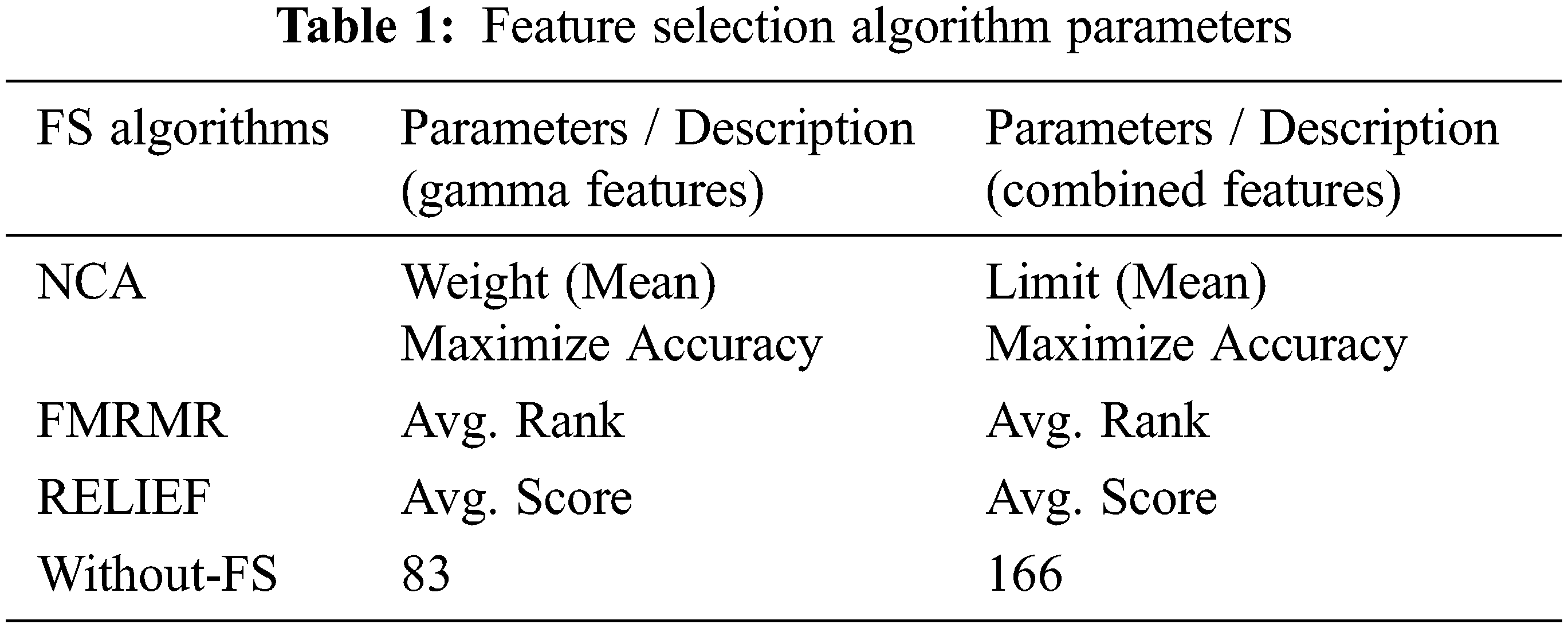
The whole sequence data contains all frames in the dataset. The performance before feature selection is compared to its performance after feature selection. The description and parameters of this block are summarized in Tab. 1.
Cross-validation using the K-fold Name and Value pair argument is a good policy in machine learning [48]. The model’s generalization ability is determined by the cross-validation results. 10-fold cross-validation is used in this research. Partitions data into ten roughly equal-sized folds at random, with one-fold being used to validate the model trained with the remaining subsets. This process is repeated 10 times, such that each fold is used exactly once for validation.
In the field of machine learning, the confusion matrix is a useful technique for model evaluation. It's a table that is generally used to describe the performance of a classification model and to identify the top-performing model. As we attempt to compare both the angle and combined methods, we will compute the confusion matrix into tables of percentages to appreciate the percentage of features that are correctly classified and those misclassified. Also, the accuracy, true positive rate (TPR), and positive predicted value (PPV) are calculated from the matrix and used for evaluation of the performance of the proposed models [49].
Some computations are made from the matrix. They include true positives TP, false negatives FN, false negatives FN, precision or positive predicted value PPV, and recall or true positive rate TPR. The above metrics will determine the model with the strongest predictors. They are expressed mathematically in Eqs. (6)–(8).
This part gives a clear and brief discussion of the experimental findings, their interpretation, and the possible experimental inferences.
3.1 Results for the Proposed Gamma Angle Feature Technique
This approach considers the combined angle and magnitude predictors derived from the geometry of the input data. The 3D geometric coordinates are extracted from the video data and all experiments are performed with and without feature selection.
3.1.1 Gamma Angles + Without-Fs (G+W)
The algorithm utilizes the entire frame sequence as well as all extracted features. In this paper, we used 48,000 samples of training data and 12,402 samples of test data. The average validation accuracy for all classes was 99.106 percent. The total cost of validation due to misclassification is 429. We achieved an average test accuracy of 99.298 percent with a total cost of misclassification of 87. The total number of features used in this model is 83, and no feature selection is required for this model. The results of the classifiers can be found in Tab. 2 (see row 3). The evaluation of each model shows that anger class 1 has the highest true positive rate TPR (99.95%), while fear class 4 has the lowest TPR (98.83%) on test data for the G+W model.
3.1.2 Gamma Angles + NCA Fs (G+N)
The algorithm achieved an overall average validation accuracy of 90.083 percent across all classes. The overall cost of validation due to misclassification is 447. We had an average test accuracy of 99.306 percent, with a total cost of misclassification of 85. The NCA algorithm identified 33 features with an average feature weight of 1.4346. Of the total 83 features, the following were included in the feature index: 7, 15, 16, 17, 19, 23, 26, 27, 33, 35, 36, 37, 38, 39, 40, 43, 44, 46, 47, 48, 55, 58, 64, 65, 68, 73, 77, 78, 79, 80, 81, 82, 83. The results of the classifiers can be found in Tab. 2 (see row 4). Evaluation by each model shows that class Anger has the maximum true positive rate TPR (99.9%), while class 4 has the least TPR (98.5%) for testing. Class 2 (disgust) on Tab. 2, row 4, column 6, shows that more of the positive results from this testing procedure are false positives.
3.1.3 Gamma Angles + FMRMR Fs (G+F)
This method achieved an average validation accuracy of 98.77 percent across all classes. The overall cost of misclassification in validation is 381, which is 0.7937 of the total training data. We achieved an average test accuracy of 99.306%, with a total cost of misclassifications of 136, which is 1.096 percent of the total test samples. The total number of features selected for training is 38. The algorithm used a mean feature importance score of 0.05 for subset feature selection. The results of the classifiers can be found in Tab. 2 (see row 5). For the testing, class 1 (sad) has the highest rate of true positive scores (100%), while class 4 (disgust) has the lowest rate of true positive scores (96.673%). Class 2 (disgust) has the lowest PPV of 96.7%, indicating that most of the positive results of this testing procedure are false positives.
3.1.4 Gamma Angles + RELIEF Fs (G+R)
The model had a validation accuracy of 94.64 percent across all classes. The overall cost of misclassification in validation is 2573, which is about 5.36 percent of the total training data. The average test accuracy was 94.75 percent, and the total cost of misclassifications in testing was 651, which is 5.249 percent of the total test samples. There are a total of 35 features that were selected for training. The algorithm used a mean feature weight of 0.0289 for subset feature selection. The feature index is as follows: 1, 3, 5, 8, 9, 10, 17, 23, 26, 27, 28, 36, 37, 38, 39, 40, 44, 45, 46, 47, 48, 49, 54, 56, 57, 60, 61, 65, 66, 67, 76, 78, 79, 80, 81. The results of the classifiers can be found in Tab. 2 (see row 6). For the test result, sad class 1 has the highest true-positive rate (98.88%), while disgust class 4 has the lowest true-positive rate (84.09%) for testing. Class 2 (disgust) has the lowest PPV of 95.23%, indicating that most of the positive results for this test procedure are false positives.
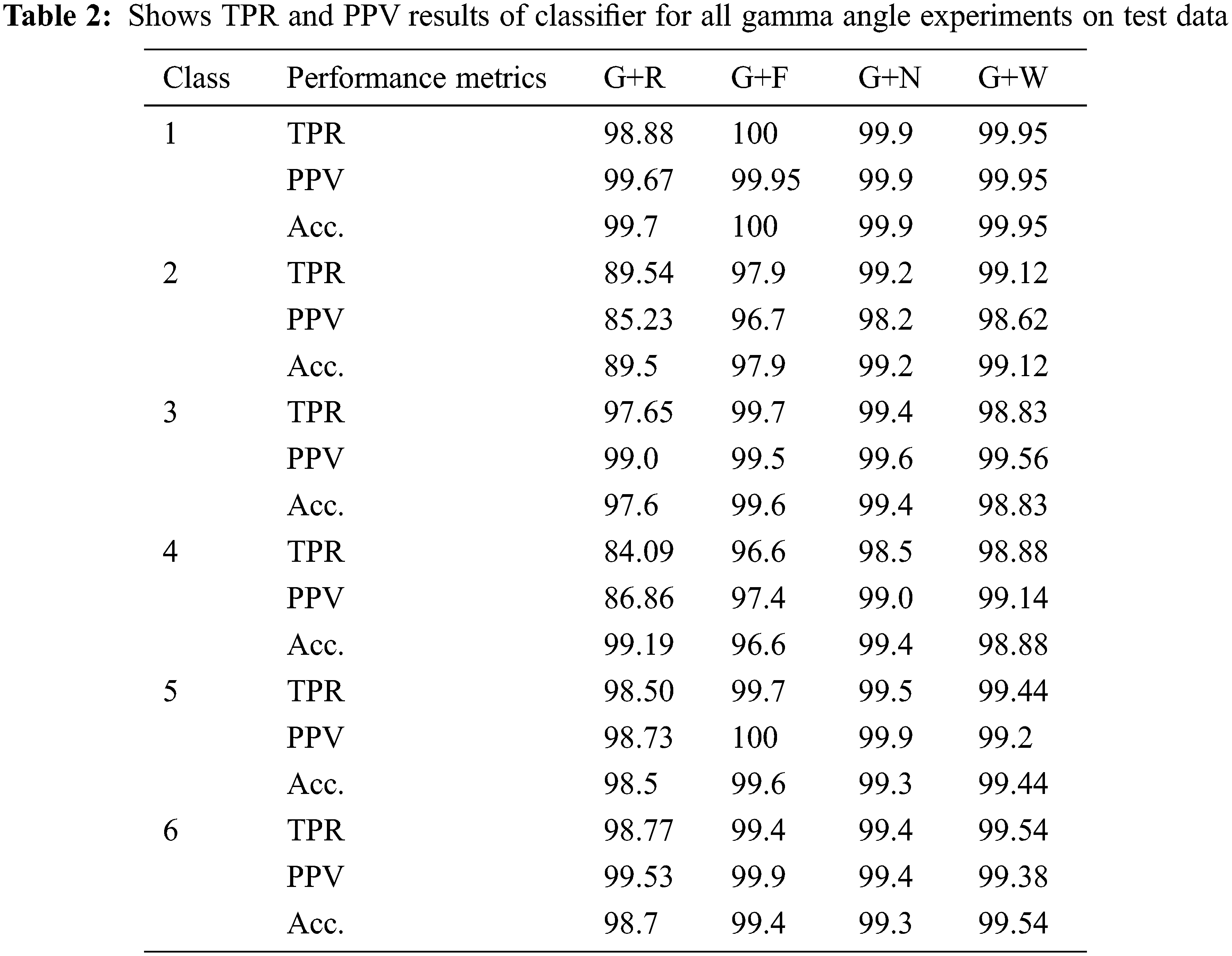
Considering Tab. 2 above, the performance per class in terms of TPR for all four gamma models (row 3: row 5) is analyzed as follows: the G+F produced the top performance in class 1 (100%), the G+N in class 2 (99.2%), the G+F in class 3 (99.7%), the G+W in class 4 (98.88%), the G+F in class 5 (99.6%), and the G+W in class 6 (99.54%). Generally, it is obvious that the G+F provides good results in classes 1, 3, and 5. G+W provides better results in classes 4 and 6.
3.2 Results for the Proposed Magnitude Feature Technique
3.2.1 Magnitude + Without-Fs (M+W)
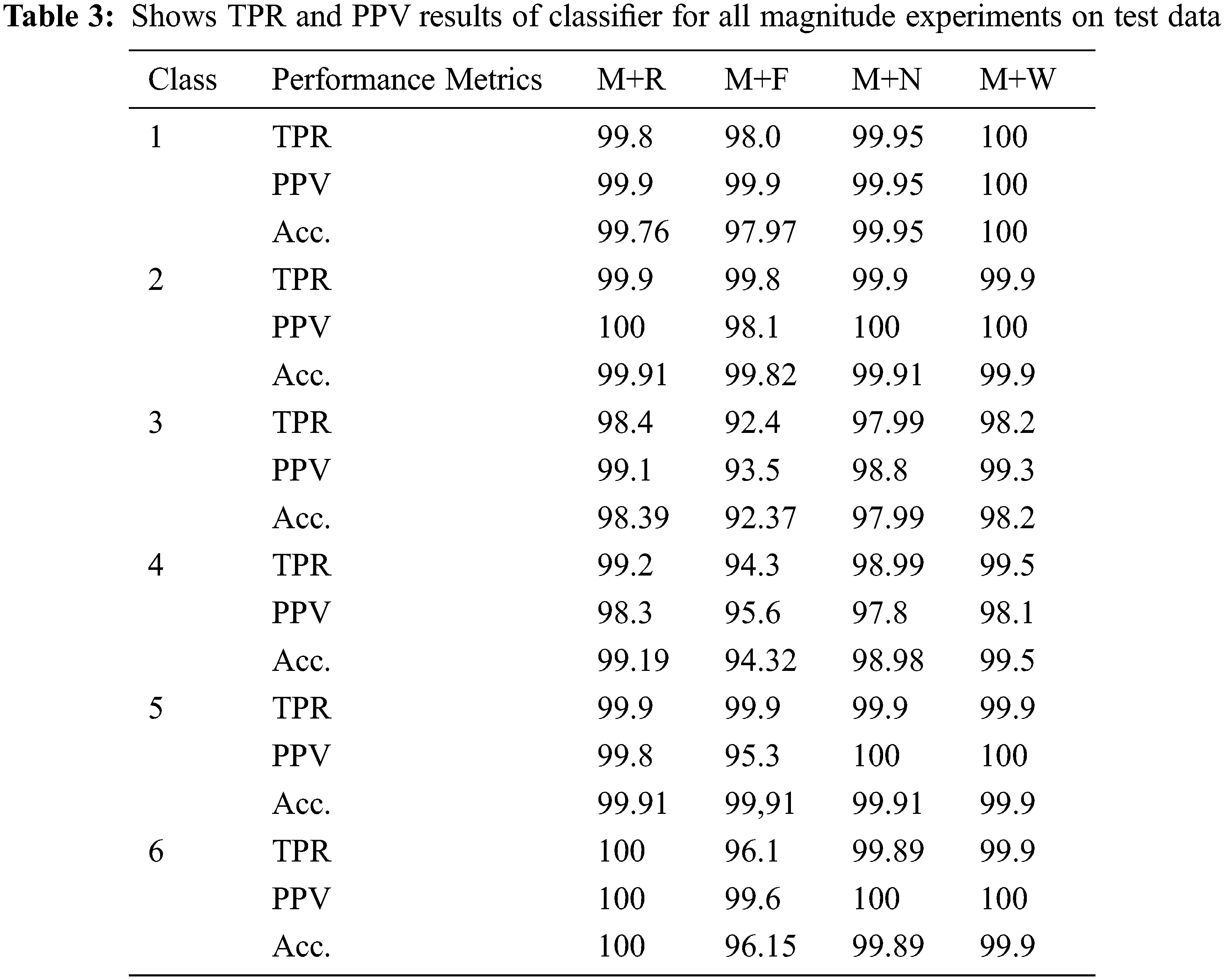
For all classes, the model achieved an average validation accuracy of 99.995 percent. The overall misclassified cost for validation is 268, or 0.5583 percent of the total training data. We achieved an average test accuracy of 99.565 percent, with a total cost of test misclassification of 53, accounting for 0.4273 percent of all test samples. There are a total of 83 features that have been chosen.
3.2.2 Magnitude + NCA Fs (M+N)
The average validation accuracy for all classes is 98.77%. The total misclassified cost for validation is 313, which accounts for about 0.652 percent of the total training data. For the testing, we obtained an average test accuracy of 99.306% and the total test misclassification cost was 136, which accounts for 1.096% of the total test samples. The total number of features selected for training is 33. The algorithm used a relative threshold of 1.2166 for subset feature selection. 3, 4, 6, 8, 13, 19, 22, 24, 27, 31, 33, 40, 43, 44, 46, 49, 50, 51, 54, 57, 58, 59, 62, 70, 72, 73, 74, 76, 79, 80, 81, 83.
3.2.3 Magnitude + FMRMR Fs (M+F)
The technique obtains a validation accuracy of 96.8% across all classes. The overall misclassified cost for validation is 1516, or 3.158 percent of the total training data. We achieved an average test accuracy of 96.839 percent, with a total test Misclassification cost of 392, accounting for 3.16 percent of all test samples. The total number of features selected is 17 for training using 0.1414. The selected feature index is as follows: 4, 5, 6, 19, 21, 22, 23, 24, 25, 28, 60, 69, 70, 71, 72, and 73.
3.2.4 Magnitude + RELIEF Fs (M+R)
The algorithm achieves an average validation accuracy for all classes of 99.37%. The total misclassified cost for validation is 306, which accounts for about 0.6375% of the total training data. For the testing, we obtained an average test accuracy of 99.53% and the total test misclassification cost is 58, which accounts for 0.467% of the total test samples. The total number of features selected for training is 24. The algorithm used a relative threshold of 0.0222 for subset feature selection.
Considering Tab. 3, performance per class in terms of TPR for all four magnitude models (row 3: row5), the M+W produced the top performance in class 1 (100%). The M+W, M+N, and M+R had a top performance of 99.9% in class 2. M+R in class 3 (98.4%), M+W in class 4 (99.5%). All four models had an equal score of TPR (99.9%) in class 5. Finally, M+R in class 6 (100%). Generally, it is obvious that the M+W provides good results in classes 1, 3, 4, and 6.
3.3 Results for the Proposed Combined Feature Model (CFM) Technique
Given the two models, SGamma and SMag., a feature model that combines both angles and magnitudes are constructed. The combination of these techniques allows us to obtain rich information about the facial expressions as depicted in Eq. (9). The feature vectors are concatenated as thus:
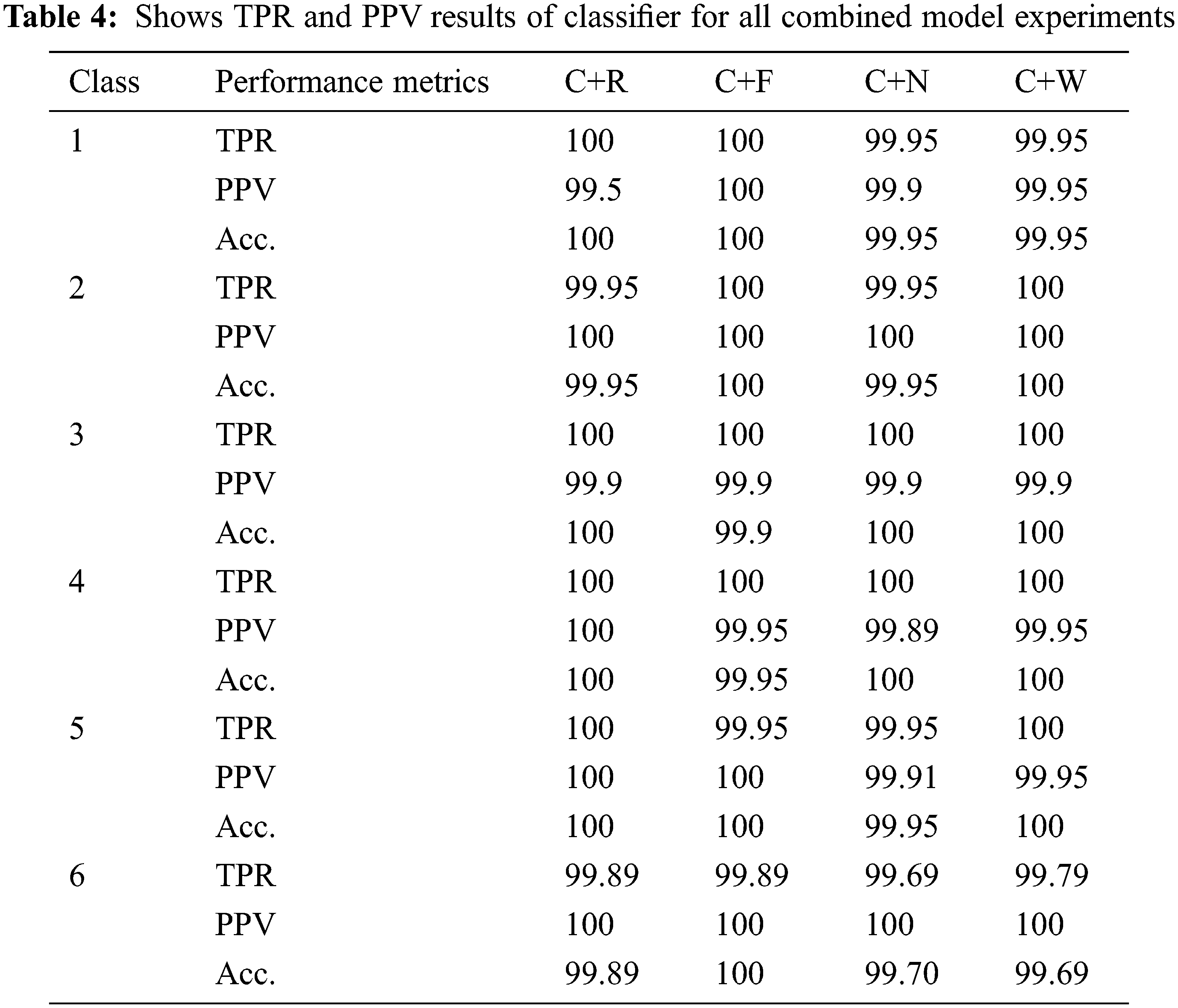
This algorithm combines the gamma and distance features without feature selection. The average validation accuracy for all classes is 99.958%, with a training sample of 48,000. The total number of misclassifications for validation is 20, which is about 0.00416 of the total training data. For the testing, we achieved an average test accuracy of 99.959% and the total misclassification cost for testing is 5, which is 0.0403% of the total test samples. The total number of combined features is 166.
For all classes, the model achieves an average validation accuracy of 99.927 percent. The overall cost of validation due to misclassification is 35. We achieved an average test accuracy of 99.93 percent, with total cost of misclassification of 9. The NCA algorithm selected 52 features with a mean feature weight of 0.5189. The selected feature index is as follows: 1, 5, 9, 10, 15, 16, 17, 31, 33, 36, 38, 39, 42, 47, 51, 55, 56, 57, 61, 66, 71, 73, 75, 76, 78, 80, 81, 83, 86, 87, 89, 102, 105, 107, 110, 111, 116, 123, 126, 127, 133, 134, 137, 141, 145, 153, 155, 157, 159, 162, 164, 166.
The model obtains optimal feature subsets by considering predictors that rank above the mean value for feature importance. The average validation accuracy for all classes is 99.943%. The total number of misclassified costs for validation is 27. For the test, we obtained an average test accuracy of 99.97% and the total misclassification cost for the test was 3. The number of features selected by the MRMR algorithm is 23, with a mean feature importance score of 0.5189. The number of features selected is 23, and the index is as follows: 38, 78, 79, 80, 81, 82, 87, 88, 89, 102, 104, 105, 106, 107, 110, 111, 143, 151, 152, 153, 154, 155, 156. Features below 83 are angle features, and indices around 83 to 166 are magnitudes. Based on the mean feature scores, only six angle features and seventeen magnitudes are selected by the proposed MRMR algorithm.
This model combines the gamma and distance predictor with the RELIEF feature selection. The average validation accuracy for all classes is 99.952%, with a training sample of 48,000. The total number of misclassified costs for validation is 23, which is about 1.002% of the total training data. For the tests, we obtained an average test accuracy of 99.975%, and the total misclassification cost for the tests was 3, which is 0.653% of the total test samples. The total number of features selected using the average mean score of 0.0322 is 67, and the algorithm uses about 40% of the total features extracted (166). Angle features are arranged in rows 1 to 83 and magnitudes in rows 84 to 166. The relief feature algorithm is applied and, based on the feature weights, the predictors with ranks above the mean tolerance are extracted. 37 angle features are selected, and 30 of those features are magnitude features. The tolerance is 0.0322 and feature indices selected are: 1, 2, 3, 4, 5, 8, 9, 10, 19, 20, 23, 26, 28, 35, 36, 37, 38, 39, 40, 44, 45, 46, 47, 48, 49, 54, 56, 57, 60, 61, 65, 66, 76, 78, 79, 80, 81, 86, 87, 88, 89, 90, 102, 104, 105, 106, 107, 123, 127, 132, 133, 134, 137, 140, 141, 142, 144, 145, 152, 153, 154, 155, 156, 158, 159, 162, 166.
The result of the gamma angle model is given in Tab. 5 (column 2:5). The G+N technique (column 3) is the model with the highest performance (99.3068%) in terms of average recognition accuracy. The G+N technique outperforms the G+W technique by 0.0118 percent, the G+F technique by 0.4168 percent, and the G+R technique by 4.594 percent. The result of the magnitude model can be seen in Tab. 5 (column 6:9). The top-performing model is the M+W technique, with an average recognition rate of 99.57%, as can be seen in Tab. 5 (column 8). M+N outperforms M+F and M+R by 0.0118%, 0.4168%, and 0.045%, respectively. Finally, the result of the combined feature model is in Tab. 5 (column 10:13). The top-performing models are the C+F and C+R techniques, with recognition rates of 99.975%. C+F and C+R outperform C+W and C+N by 0.034% and 0.045%, respectively. Considering all models, the overall top-performing model is the C+F and C+R technique as shown in Tab. 4.

In machine learning, model complexity often refers to the number of features or terms included in a given predictive model. The information contained in the last two rows of Tab. 5 provides a rough estimate of the complexity of the model. It is clear that using a reduced feature subset or fewer predictors will mean less computation during training and testing in real-time applications. The result also explains the importance of feature selection in improving the general classifier performance. For the gamma feature model, the model G+N achieved a higher ARR of 99.306% than the model without feature selection, G+W, whose ARR is 99.29%. For the combined feature model, the model without-Fs (C+W) achieved an ARR of 99.941% (see Tab. 5, column 10) as against 99.975% achieved by the model with optimal feature subset selection (C+F & C+R). This is a 0.034% improvement over ARR.
However, the concept of computational complexity relates mostly to how the input size (n) of an algorithm relates to the number of operations. Based on the direct proportional rate of growth experienced in all the stages of the proposed framework, a rough estimate of the complexity would be in linear time O (n). In this situation, we take a look at every frame in the sequence or visit every feature element selected to accomplish the task. The complexity of the system can be analyzed according to the dataset used. First of all, the BU-4DFE dataset uses manual labeling of geometric landmarks and then employs an Active Appearance Model (AAM) for the tracking of these geometric features for the rest of the frames. Thus, complexity is inherited from the dataset itself. Considering the time complexity, tracking of geometric features can be analyzed. According to the AAM method, the first average model fitting can be done, denoted by the projection p. The appearance model is learned by first warping each of the training images, and then the shape model is typically learned by annotating N fiducial points. Generalizing this process may result in a time complexity of O (pN) per frame [50].
One has two goals at this point: one is to minimize the number of geometric features used and the other is to minimize the number of frames processed. In this paper, the number of feature points can be monitored in Tab. 5. Future work can be done on the optimization of frames and the application of frame selection. On the other hand, the system’s space complexity is also significant. In this dataset, each 3D model of a video sequence has a resolution that includes about 35,000 vertices. The texture video includes about 1040 × 1329 pixels per frame. The resulting dataset is roughly 500 Gigabytes. The video files for every expression are captured for about 4 seconds. Considering this setup, 4 seconds can be the buffering memory size for the overall expressions in real time. As this is for 101 subjects and 7 expressions (including the neutral) [15], considering only the testing, roughly 1 Gigabyte of space will be enough to store necessary features.
From the perspective of model type and methodology, we first discuss our findings in existing studies. Then, we perform a unified evaluation of recognition accuracy and identify the top performing model(s).
Based on the results of our tests, it is clear that our proposed method can effectively cope with 4D face expression recognition. In this research, we proposed a new framework for expression recognition from 3D dynamic images (video) using an axes-angle feature-based method. The axes-angle and magnitude predictors extracted using descriptors with varied qualities were combined by concatenating the resulting feature vectors. In this study, a 4-D facial expression network is configured to process spatio-temporal data, and then the data is split into test and training sets by 10-fold cross validation (10-CV) for all experiments.
Tab. 6 displays the overall result for all methods prior to, with, and without feature selection. SVM benefits from scaling of data (z-score), as after scaling there was a dramatic improvement in accuracy. The SVM model is more sensitive to variables with large variance and less sensitive to variables with small variance. The ideal kernel width is generally close to 1 when variables are normalized. In Tab. 7, the models with the best recognition accuracy are compared to state-of-the-art approaches.


Using manual landmark features from the CK database, the authors of [51] achieved 99.58 percent accuracy. In the study, the author also employed a 3D model known as the Candide wireframe and tried to track the changes in geometric points. Mainly, they used the 3D distances between the points to detect the facial expressions. By comparing this study with our proposed approach, it seems that the proposed approach also considers the angles between the points, furthermore concatenating the angle with 3D distance information. Thus, the feature vectors are enriched. Furthermore, the proposed method uses 3D distance and angles instantly, whereas in [51], they used 3D model-assisted landmark tracking., both approaches achieved a high recognition rate.
The top-performing model is the combined method as shown in Tab. 7. It outperforms distance-based methods used in [53], as well as other techniques not included in Tab. 7 that use still images and the apex of the expressions [56,57]. Also, in [54,55], though the author’s included angles between features, our method produced superior recognition accuracy. Their method has resulted in 87.05% and 83.5%, respectively, as against the 99.975% produced by both the C+F and C+R techniques. For FER systems, specifically for dynamic facial expression recognition, one of the main phases that carries high computational and time complexity is feature extraction. We implemented a filter-based feature selection strategy, and it can be argued that the proposed low-complexity approach is effective. Fig. 4 visually clarifies the performance trends better than the result table. The diagram shows how the models in the line chart perform in terms of the various predictor types. When compared to the other models, it is clear that the combined model has great performance.

Figure 4: Performance trend of all proposed methods on the BU-4DFE dataset for 4D FER
The line chart suggests that it is possible to implement feature reduction while maintaining a tolerance in accuracy of ±5.2% when compared to the result obtained from a model without feature selection.
The diagram shows how the feature selection framework affects the model complexity. Basically, the use of fewer features reduces model complexity and requires minimal computing resources. The clustered bar in Fig. 5 provides a visual explanation of the model with fewer features to compute. M+R appears to have the lowest value, with 17 predictors accounting for 20% of the total feature.

Figure 5: Feature size for different models
In this paper, the overall goal was to design a classification pipeline to automatically classify video file-based emotions expressed. Three main approaches were analyzed to achieve that goal, which are the gamma angle-based method, the magnitude or distance-based method, and the combined method. The entire experiments were carried out using the BU4DFE dataset. According to the results obtained, the maximum overall accuracy achieved was 99.975% using the combined angle method, as against 99.307% obtained for gamma angle methods and 99.756% for the magnitude methods. It seems clear that our CFM proposal for facial expression recognition outperforms the gamma angle or magnitude approach when used separately, with or without feature selection. Moreover, our approach can classify faces from different ethnic groups, i.e., people independently, giving an accurate expression recognition result. Then it becomes pertinent to emphasize that the novelty of this paper is built on using angle information extracted from the geometric feature points on the face. The main advantage of this kind of approach is that it creates a robust feature space; that is, the angles are invariant to translations and rotations of the faces. After necessary experiments are conducted on this idea, it is shown that the proposed method outperforms the other methods on the BU-4DFE dataset and produces comparable results. Furthermore, concatenating angle information with the magnitude information brings a slight improvement in the overall accuracies reported.
Future work could be about exploring other 3D axes for feature extraction (alpha & beta angles), modifying the feature selection block to include tuning the regularization parameter in NCA, using cross-validation to correctly detect the relevant features in the data, and using Bayesian optimizers for classifier hyper-parameter search are all possibilities for future work. It's possible to implement a real-time peak entropy key frame selection algorithm that selects just high intensity or peak frames per second to reduce complexity in dynamic 4D FER, and better expression recognition performance may be achieved.
Acknowledgement: This paper was supported by Cyprus International University, whose library resources proved relevant to achieving the research objectives.
Funding Statement: The authors received no specific funding for this study.
Conflicts of Interest: The authors declare that the research was conducted in the absence of any commercial or financial relationships that could be construed as a potential conflict of interest.
1. D. Fabiano and S. Canavan, “Spontaneous and non-spontaneous 3D facial expression recognition using a statistical model with global and local constraints,” in Proc. the 25th IEEE Int. Conf. on Image Processing (ICIP), Athens, Greece, pp. 3089–3093, 2018. [Google Scholar]
2. M. S. Bartlett, J. C. Hager, P. Ekman and T. J. Sejnowski, “Measuring facial expressions by computer image analysis,” Psychophysiology, vol. 36, no. 2, pp. 253–263, 1999. [Google Scholar]
3. C. Darwin and F. Darwin, “The expression of the emotions in man and animals,” 2nd ed., John Murray, London,1904 [Online]. Available:http://darwin-online.org.uk/content/frameset?pageseq=1&itemID=F1142 [Google Scholar]
4. P. Ekman and W. V. Friesen, “Constants across cultures in the face and emotion,” Journal of Personality and Social Psychology, vol. 17, no. 2, pp. 124–129, 1971. [Google Scholar]
5. P. Ekman and W. V. Friesen, “Unmasking the face: A guide to recognizing emotions from facial clues,” Institute of the Study of Human Knowledge. Los Altos: CA Malor Books, 2003. [Google Scholar]
6. P. Zarbakhsh and H. Demirel, “Fuzzy SVM for 3D facial expression classification using sequential forward feature selection,” in Proc. 9th Int. Conf. on Computational Intelligence and Communication Networks (CICN), Girne, Northern Cyprus, pp. 131–134, 2017. [Google Scholar]
7. J. J. J. Lien, T. Kanade, J. F. Cohn and C. C. Li, “Detection, tracking, and classification of action units in facial expression,” Robotic Automation System, vol. 31, no. 3, pp. 131–146, 2000. [Google Scholar]
8. Y. Tian, T. Kanade and J. F. Cohn, “Recognizing action units for facial expression analysis,” IEEE Transactions on Pattern Analysis and Machine Intelligence, vol. 23, no. 2, pp. 97–115, 2001. [Google Scholar]
9. G. Abrantes and F. Pereira, “MPEG-4 facial animation technology: Survey, implementation and results,” IEEE Transactions on Circuits and Systems for Video Technology, vol. 9, no. 2, pp. 290–305, 1999. [Google Scholar]
10. M. S. Bartlett, G. Littlewort, M. G. Frank, C. Lainscsek, I. R. Fasel et al., “Automatic recognition of facial actions in spontaneous expressions,” Journal of Multimedia, vol. 5, no. 6, pp. 22–35, 2006. [Google Scholar]
11. M. Romero and N. Pears, “Landmark localization in 3d face data,” in Proc. Sixth IEEE Int. Conf. on Advanced Video and Signal Based Surveillance, Genova, Italy, pp. 73–78, 2009. [Google Scholar]
12. D. Jeong, B. G. Kim and S. Y. Dong, “Deep joint spatiotemporal network (djstn) for efficient facial expression recognition,” Sensors, vol. 20, no. 2, pp. 297–307, 1939. [Google Scholar]
13. B. B. Amor, H. Drira, S. Berretti, M. Daoudi and A. Srivastava, “4D facial expression recognition by learning geometric deformations,” IEEE Transactions on Cybernetics, vol. 44, no. 12, pp. 2443–2457, 2014. [Google Scholar]
14. M. Behzad, N. Vo, X. Li and G. Zhao, “Automatic 4d facial expression recognition via collaborative cross-domain dynamic image network,” in British Machine Vision Conf. on Computer Vision, Cardiff, UK, pp. 364–365, 2019. [Google Scholar]
15. L. Yin, X. Chen, Y. Sun, T. Worm and M. Reale, “A high-resolution 3D dynamic facial expression database,” in Proc. 8th IEEE Int. Conf. on Automatic Face & Gesture Recognition, Amsterdam, Netherlands, pp. 1–6, 2008. [Google Scholar]
16. Y. Sun and L. Yin, “Facial expression recognition based on 3D dynamic range model sequences,” in Proc. the 10th European Conf. on Computer Vision (ECCV08), Marseille, France, pp. 12–18, 2008. [Google Scholar]
17. M. Murugappan and A. Mutawa, “Facial geometric feature extraction-based emotion expression classification using machine learning,” PLoS ONE, vol. 16, no. 2, pp. 1371–1374, 2021. [Google Scholar]
18. G. Sandbach, S. Zafeiriou, M. Pantic and D. Rueckert, “Recognition of 3D facial expression dynamics,” Image and Vision Computing, vol. 30, no. 44, pp. 762–773, 2012. [Google Scholar]
19. S. Canavan, Y. Sun, X. Zhang and L. Yin, “A dynamic curvature-based approach for facial activity analysis is 3D space,” in Computer Vision and Pattern Recognition Workshops, pp. 3416, 2012. [Google Scholar]
20. V. Le, H. Tang and T. S. Huang, “Expression recognition from 3D dynamic faces using robust spatio-temporal shape features,” in proc. of the Face and Gesture, Santa Barbara, CA, USA, pp. 414–421, 2011. [Google Scholar]
21. T. Fang, X. Zhao, O. Ocegueda, S. K. Shah and I. A. Kakadiaris, “3d/4d facial expression analysis: An advanced annotated face model approach,” Image and Vision Computing, vol. 30, no. 10, pp. 738–749, 2012. [Google Scholar]
22. Q. Zhen, D. Huang, Y. Wang and L. Chen, “Muscular movement model-based automatic 3D/4D facial expression recognition,” IEEE Transactions Multimedia, vol. 18, no. 7, pp. 1438–1450, 2016. [Google Scholar]
23. Y. Sun, M. Reale and L. Yin, “Recognizing partial facial action units based on 3D dynamic range data for facial expression recognition,” in Proc. of the 8th IEEE Int. Conf. on Automatic Face Gesture Recognition, Amsterdam, The Netherlands, pp. 1–8, 2008. [Google Scholar]
24. K. Yurtkan and H. Demirel, “Feature selection for improved 3D facial expression recognition,” Pattern Recognition Letter, vol. 38, no. 1, pp. 26–33, 2014. [Google Scholar]
25. N. Francesca, D. Nicole, M. Federica and V. Enrico, “3D approaches and challenges in facial expression, recognition algorithms - A literature review,” Applied Sciences, vol. 9, no. 18, pp. 3904, 2019. [Google Scholar]
26. R. Srivastava and S. Roy, “Utilizing 3D flow of points for facial expression recognition,” Multimedia Tools and Applications, vol. 71, no. 3, pp. 1953–1974, 2014. [Google Scholar]
27. M. Hayat and M. Bennamoun, “An automatic framework for textured 3D video-based facial expression recognition,” IEEE Transactions on Affective Computing, vol. 5, no. 3, pp. 301–313, 2014. [Google Scholar]
28. S. Shilpi and S. V. A. V. Prasad, “Techniques and challenges of face recognition: A critical Review,” Procedia Computer Science, ScienceDirect, vol. 143, pp. 536–543, 2018. [Google Scholar]
29. K. Bowyer, K. Chang and P. Flynn, “Á survey of approaches and challenges in 3d and multi-modal 3d+2d face recognition,” Computer Vision and Image Understanding, vol. 101, no. 1, pp. 1–15, 2006. [Google Scholar]
30. S. J. B. Lawrence, “3D and 4D face recognition: A comprehensive review,” Recent Patents on Engineering, vol. 8, no. 2, pp. 112–119, 2014. [Google Scholar]
31. I. Kakadiaris, G. Passalis, G. Toderici, M. Murtuza and T. Theoharis, “3D face recognition,,” in British Machine Vision Conf. (BMVC), pp. 869–878, 2006. [Google Scholar]
32. A. Maalej, B. B. Amor, M. Daoudi, A. Srivastava and S. Berretti, “Local 3D shape analysis for facial expression recognition,” in Proc. of the 20th Int. Conf. on Pattern Recognition, Istanbul, Turkey, pp. 4129–4132, 2010. [Google Scholar]
33. S. Arman, S. BuLent and M. Taha, “Comparative evaluation of 3D vs 2D modality for automatic detection of facial action units,” Pattern Recognition, vol. 45, no. 2, pp. 767–782, 2012. [Google Scholar]
34. S. Li and W. Deng, “Deep facial expression recognition: A survey,” in Computer Vision and Pattern Recognition, 2018 [Online]. Available:https://arxiv.org/abs/1804.08348 [Google Scholar]
35. Z. Xiaoliang, Y. Shihao, Z. Liang and D. Zhicheng, “Hybrid attention cascade network for facial expression recognition,” Sensors, vol. 21, no. 6, pp. 1231, 2021. [Google Scholar]
36. B. Hasani and M. H. Mahoor, “Facial expression recognition using enhanced deep 3D convolutional neural network,” in IEEE Conf. on Computer Vision and Pattern Recognition Workshops (CVPRW), pp. 2278–2288, 2017. [Google Scholar]
37. J. Shao and Y. Qian, “Three convolutional neural network models for facial expression recognition in the wild,” Neurocomputing, vol. 355, no. C, pp. 82–92, 2019. [Google Scholar]
38. G. Huong and C. Jiayou, “Dynamic facial expression based on resnet and LSTM,” IOP Conference Series. Materials Science and Engineering, Bristol, vol. 790, no. 1, pp. 463, 2020. [Google Scholar]
39. S. Arnold, A. Hans and R. A. Smitha, “CNN-LSTM based deep neural network for facial emotion detection in videos,” International Journal of Advanced Science and Technology, vol. 7, no. 1, pp. 2446, 2021. [Google Scholar]
40. L. Yin, X. Chen, Y. Sun, T. Worm and M. Reale, “A high-resolution 3D dynamic facial expression database,” in Proc. 8th IEEE Int. Conf. on Automatic Face & Gesture Recognition, Amsterdam, Netherlands, pp. 1–6, 2008. [Google Scholar]
41. S. R. Jannat, D. Fabiano, S. J. Canavan and T. J. Neal, “Subject identification across large expression variations using 3D facial landmarks,” in Int. Conf. on Pattern Recognition Workshops, Milan, Italy, pp. 2122, 2020. [Google Scholar]
42. H. Soyel, U. Tekguc and H. Demirel, “Application of NSGA-II to feature selection for facial expression recognition,” Computers & Electrical Engineering, vol. 37, no. 6, pp. 1232–1240, 2011. [Google Scholar]
43. P. Ekman and W. Friesen, “Facial Action Coding System: A Technique for the Measurement of Facial Movement,” Palo Alto: Consulting Psychologists Press, 1978. [Google Scholar]
44. W. Yang, K. Wang and W. Zuo, “Neighborhood component feature selection for high-dimensional data,” Journal of Computers, vol. 7, no. 1, pp. 31–37, 2012. [Google Scholar]
45. Y. Saeys, I. Inza and P. Larra, “A review of feature selection techniques in bioinformatics,” Bioinformatics, vol. 23, no. 19, pp. 2507–2517, 2007. [Google Scholar]
46. P. Hanchuan, L. Fuhui and D. Chris, “Feature selection based on mutual information: Criteria of max-dependency, max-relevance, and min-redundancy,” IEEE Transactions on Pattern Analysis and Machine Intelligence, vol. 27, no. 8, pp. 1226–1238, 2005. [Google Scholar]
47. M. Robnik-Sikonja and I. Kononenko, “Theoretical and empirical analysis of ReliefF and RReliefF,” Machine Learning, vol. 53, no. 1/2, pp. 23–69, 2003. [Google Scholar]
48. K. Pal and B. V. Patel, “Data classification with k-fold cross validation and holdout accuracy estimation methods with 5 different machine learning techniques,” in Proc. Fourth Int. Conf. on Computing Methodologies and Communication (ICCMC), Erode, India, pp. 83–87, 2020. [Google Scholar]
49. R. Susmaga, “Confusion Matrix Visualization,” Intelligent Information Processing and Web Mining, part of the Advances in Soft Computing, vol. 25, pp. 107–116, 2004. [Google Scholar]
50. G. Tzimiropoulos, J. Alabort-i-Medina, S. Zafeiriou and M. Pantic, “Generic active appearance models revisited,” in Proc. of Asian Conf. on Computer Vision, Berlin, Heidelberg, Springer, pp. 650–663, 2012. [Google Scholar]
51. I. Kotsia and I. Pitas, “Facial expression recognition in image sequence using geometric deformation features and support vector machines,” IEEE Transactions on Image Processing, vol. 16, no. 1, pp. 172–187, 2007. [Google Scholar]
52. G. Deepak and L. Joonwhoan, “Geometric feature-based facial expression recognition in image sequences using multi-class ada-boost and support vector machines,” Sensors, vol. 13, no. 6, pp. 7714–7734, 2013. [Google Scholar]
53. P. Zarbakhsh and H. Demirel, “Fuzzy SVM for 3D facial expression classification using sequential forward feature selection,” in Proc 9th Int. Conf. on Computational Intelligence and Communication Networks (CICN), Girne, Northern Cyprus, pp. 131–134, 2017. [Google Scholar]
54. O. K. Oyedotun, G. Demisse, R. S. El, D. Aouada and B. Ottersten, “Facial expression recognition via joint deep learning of RGB-Depth map latent representations,” in Proc. of IEEE Int. Conf. on Computer Vision Workshops, (ICCVW), Venice, Italy, pp. 3161–3168, 2017. [Google Scholar]
55. P. Zarbakhsh and H. Demirel, “4D facial expression recognition using multimodal time series analysis of geometric land-mark-based deformations,” Visual Computer, vol. 20, pp. 951–965, 2020. [Google Scholar]
56. H. Soyel, U. Tekguc and H. Demirel, “Application of NSGA-II to feature selection for facial expression recognition,” Computers & Electrical Engineering, vol. 37, no. 6, pp. 1232–1240, 2011. [Google Scholar]
57. H. Tang and T. S. Huang, “3D facial expression recognition based on properties of line segments connecting facial feature points in Proc,” in Proc. of 8th IEEE Int. Conf. on Automatic Face and Gesture Recognition, FG, Amsterdam, Netherlands, pp. 1362, 2008. [Google Scholar]
 | This work is licensed under a Creative Commons Attribution 4.0 International License, which permits unrestricted use, distribution, and reproduction in any medium, provided the original work is properly cited. |