DOI:10.32604/iasc.2022.025192
| Intelligent Automation & Soft Computing DOI:10.32604/iasc.2022.025192 | |
| Article |
Modeling Metaheuristic Optimization with Deep Learning Software Bug Prediction Model
1Department of Computer Science and Engineering, Sathyabama Institute of Science and Technology, Chennai, 600 0119, India
2Department of Computer Science and Engineering, Panimalar Engineering College, Chennai, 600 123, India
*Corresponding Author: M. Sangeetha. Email: sangeethameckanzi2224@gmail.com
Received: 15 November 2021; Accepted: 09 February 2022
Abstract: Software testing is an effective means of verifying software stability and trustworthiness. It is essential in the software development process and needs a huge quantity of resources such as labor, money, and time. Automated software testing can be used to save manual work, shorten testing times, and improve testing performance. Recently, Software Bug Prediction (SBP) models have been developed to improve the software quality assurance (SQA) process through the prediction of bug parts. Advanced deep learning (DL) models can be used to classify faults in software parts. Because hyperparameters have a significant impact on the performance of any DL model, a proper hyperparameter optimization approach utilizing metaheuristic methods is required. This paper provides a unique Metaheuristic Optimization with Deep Learning based SBP (MODL-SBP) methodology to ensure software dependability and trustworthiness. The suggested technique entails creating a hybrid Convolution Neural Network (CNN) bi-directional long short-term memory (BiLSTM) to forecast software problems. Furthermore, the Chaotic Quantum Grasshopper Optimization Algorithm (CQGOA) is used for hyperparameter optimization of the CNN-BiLSTM models, which enhances predictive accuracy. To demonstrate the superior performance of the MODL-SBP technique, a wide range of simulations are performed on benchmark datasets, with the results highlighting the superior performance of the proposed model over other recent techniques.
Keywords: Software testing; software bug prediction; deep learning; metaheuristics; hyperparameter tuning
The software application’s influence is growing with time. Effort estimation is the fastest developing field in business and academia [1]. Because the total cost and duration of software testing are increasing daily, the key problem for software practitioners and academics is to improve software quality while utilizing limited testing resources. The main goal of the Software Bug Prediction (SBP) approach is to categorize fault-free and faultily models, and then the developer would allocate testing preferences of many software components, assign appropriate testing sources, and improve software quality [2]. A software bug is a flaw, defect, or error that results in unexpected or erroneous results [3]. Because resources are limited, software components with flaws should be prioritized. SBP approaches for detecting bug-prone software components using machine learning (ML) classifier algorithms were presented to address resource allocation challenges. SBP is an essential topic in software development since anticipating errors in software systems improves quality and hence reduces work and maintenance costs. SBP enables SQA teams to detect defects in problematic code throughout the software development process, preventing them from producing additional errors in other areas of the programme components/modules.
SBP is an important part of software development. This is because predicting the malfunctioning components prior to programme launch promotes customer satisfaction and improves overall software performance. Furthermore, predicting software problems increases resource usage and enhances programme adaptation to various contexts [4]. Several techniques to coping with SBP concerns have been offered. Machine Learning (ML) techniques are the most often utilized in SBP for forecasting problematic components based on significant metrics, various software computing strategies, and historical fault data [5]. A hyperparameter is an ML classification parameter that has been altered to improve prediction/performance accuracy. In general, hyperparameter optimization is the process of fine-tuning the hyperparameters of ML techniques or determining the optimal hyperparameter values; it is sometimes referred to as hyper-parameter tuning or model selection. Various classifications have different properties that must be improved for the hyperparameter to improve [6]. In previous decades, publications provided several approaches for analysing the performance of ML classifiers in software bug prediction [7].
Machine learning (ML) is a subset of deep learning (DL) (ML). DL tries to reflect higher-level abstraction in data using numerous processing layers and sophisticated structures based on a set of models [8]. Deep learning (DL) refers to a class of models and techniques that include, but are not limited to, Deep Belief Networks (DBN), Convolution Neural Networks (CNN), Deep Boltzmann Machines (DBM), Restricted Boltzmann Machines (RBM), deep representation, and recursive auto-encoders [9]. CNN, RBM, and DBN are the most often used ML techniques for image categorization. Deep learning is distinguished from commonly used “shallow learning” approaches such as boosting, maximum entropy approach, and support vector machine by the term “Deep” (SVM). Because shallow learning primarily harvests feature through empirical/artificial sampling, the network/model would learn non-layer structural aspects [10]. DL, on the other hand, learns raw information layer by layer by shifting input from raw to changed feature space. Deep structure may be able to learn and approach non-linear functions as well.
This research offers a new metaheuristic optimization model for software testing that incorporates deep learning-based SBP (MODL-SBP). To implement the SBP as a prediction technique, the MODL-SBP approach employs a hybrid convolution neural network (CNN) bi-directional long short-term memory (BiLSTM). Furthermore, the chaotic quantum grasshopper optimization algorithm (CQGOA) is employed to optimise the CNN-BiLSTM models’ hyperparameters, which improves prediction accuracy. A wide range of simulations are run to investigate the improved efficiency of the MODL-SBP technique, and the results are evaluated in a variety of ways.
JDA-ISDA is a ground-breaking cross-project ARB prediction method developed by Arun et al. [11] that is based on Joint Distribution Adaptation (JDA) and Improved Subclass Discriminant Analysis (ISDA) (ISDA). The basic idea behind JDA-ISDA is to use JDA to lessen conditional and marginal distribution changes while employing ISDA to avoid serious class imbalance concerns. Khan et al. [12] proposed a method for detecting software defects that employs both an ML classifier and the Artificial Immune Network (AIN) to increase bug forecasting accuracy through hyperparameter tweaking. For this objective, seven ML classifications were used: KNN (Minkowski metric), SVM Radial base function (SVM-RBF), KNN (Euclidean metric), AdaBoost, NB, DT, LDA, and RF.
Pandey et al. [13] focused on proving the benefits of the FS and ML approaches for distinguishing between non-faulty and defective software components. They demonstrated fundamental SBP classifications based on Ensemble Learning and Bug Prediction with Deep Representation (BPDET). Both the DR and EL processes make use of it. Rajaram et al. [14] created the BugHunter Data Collection, which is a new type of manually built and open-source bug dataset made up of code components (files, classes, models) containing a greater range of bug information and code metrics. Another available bug dataset collects the characteristics of each source code component (non-buggy and buggy) at many pre-selected release versions of the code using the standard method.
To broaden the original dataset throughout the CNN efforts, Chaubey et al. [15] constructed the PROMISE Source Code (PSC) datasets, which were called the Simplified PROMISE Source Code (SPSC) datasets by its developer. In the data sets, each variant was used. The proposed model employs CNN hybridization with various activation functions via global pooling and is thus trained through additional tree classifications. Venu et al. [16] improved classification performance by using developed GWSO as a classification FS approach. Furthermore, rather than recognizing it as non-defective/faulty, software error detection is expected to assume the nature of the issue when rectifying it for corrective action.
Qu et al. [17] looked into the direct relationship between the various designers and the risk of a faulty file. According to an experimental investigation on nine publicly available Java systems with thirty-two versions, they uncovered an unexpected and widely recognized trend: if there are many individuals working on a source file, there is a high likelihood that this file will be problematic. Pretty Diana Cyril et al. [18] presented a function-level JavaScript issue detection system based on static source code metrics as well as hybrid (dynamic and static) code analysis-based metrics of various outgoing and incoming function calls (HNOI and HNII). Because JavaScript is a very dynamic scripting language, static code analysis may be incorrect; thus, relying solely on static source code features for issue prediction may be insufficient. Qu et al. [19] carried out an experimental investigation to evaluate network embedding strategies in bug predictions by expanding and implementing node2defect, a recently reported bug predictive strategy that concatenates the embedded vector with typical software engineering metrics. Seven network embedding approaches, two effort-aware methods, and thirteen publicly available Java schemes are used in the experiment.
In this work, a novel MODL-SBP approach was developed to predict the presence of software faults, ensuring software dependability and trustworthiness. The suggested MODL-SBP technique addresses the SBP as a classification problem that is solved with DL models. The suggested MODL-SBP technique is divided into two stages: CNN-BiLSTM prediction and CQGOA hyperparameter tuning. Fig. 1 depicts the entire method of the proposed MODL-SBP approach. The following sections go through these two techniques in further depth.

Figure 1: Overall process of MODL-SBP technique
The proposed method illustrates how the pre-processed data is originally developed using that data has normalization from zero to one since it is utilized to increase the classifier accuracy. The equation of pre-processed normalized data is shown below.
where x' denotes the variable x's normalization value, x denotes the variable x's current value, xmin denotes the dataset’s minimum data point, and xmax denotes the dataset's maximum data point. After normalization, trained data was used to train the classifier, and test data was used to compute classification accuracy. If the classification accuracy and AUC are obtained, the FF is determined using the classifier's classification accuracy, including the AUC and hyper-parameter.
3.2 Process Involved in the CNN-BiLSTM Based Prediction
The MODL-SBP approach primarily employs the CNN-BiLSTM model to forecast the emergence of software problems. The CNN BiLSTM is a unique hybrid approach combining CNN and BiLSTM, is given in this paper. The model given here has been trained to categorize a multivariate temporal sequence of land cover into its many classes. The current technique differs from conventional classification methods by including embedded relationships and efficient features in a longer time sequence, resulting in an improvement in classifier performance. The two ways mentioned above are extensively discussed below.
CNN is a kind of multilayer NN that is made up of two primary parts [20]. Initially, feature extractors learn features automatically from data. Following that, trainable FC-MLP conducts the classification algorithm based on the previously learnt feature. Typically, the feature extractor involves a number of comparable steps, all of which include pooling, filtering, and activation layers. Every layer’s output is referred to as a feature map.
A recurrent Neural Network (RNN) is a kind of ANN that differs from NNs based on feed forward by the possibility of using its internal state (memory) to handle a succession of inputs. Recently, the LSTM network has emerged as a revolutionary RNN model that addresses the concerns of the prior RNN’s vanishing gradient and holds the LSTM. The LSTM is distinguished from RNN by two characteristics. Firstly, the cell state is separated into the short-term state h(t) and the long-term state c(t). Next, an LSTM consist of output, forget, and input gates, each of which is along the state path for regulating the cell state as presented in [21].
It learns Bi-LSTM dependencies between time steps of a time sequence and is useful for a network that should be taught at all time-steps of a complete time series. With two sublayers, BiLSTM processes the input sequence in all directions. It has two recurrent network layers, the first of which handles the order of inputs in the forward direction, and the second of which handles the input sequence in the reverse direction. The two layers are coupled to a similar output layer, and the BiLSTM network obtains overall data regarding future and prior data point sequences. Both layers calculate backward and forward hidden sequences
In which:
CNN-BiLSTM, a hybrid technique combining CNN and BiLSTM networks, is described for the classification of multivariate time sequences of land cover information. The proposed model incorporates multilayers that include the proposed convolution and BiLSTM layers, as well as the FC layer, classification layer, and softmax layer. A sequence of folding layers is placed before the convolution layer to execute the convolution operation on each time step independently. A series of unfolding and flatten layers are inserted between the convolution and BiLSTM layers to restore the sequence model and reshape the output of the convolution layer to the sequence of feature vectors. The structure of the Bi-LSTM approach is seen in Fig. 2. The following depicts the different layers and parameter values of the provided model:
• A series input layer with an input size of dimension [10231]
• Series Folding Layer
• CNN includes ReLU, convolution and BN layers with multiple filters equal to 30 and with filter size of 5-by-5. 2 sequences of the layers are utilized by the presented model
• Series of Unfolding Layer restore the series model of input data afterward series folding
• Flatten Layer
• BiLSTM with 350 hidden units which output only the final time step
• An FC layer of size 9 i.e., multiple classes followed by a classification and softmax layers

Figure 2: Framework of BiLSTM
3.3 Hyperparameter Optimization Using CQGOA
The CQGOA is used to successfully tune the CNN-BiLSTM model’s hyperparameters. The GOA is a revolutionary SI-based metaheuristic technique inspired by the extended range and quick movement of adult grasshoppers in groups. The metaheuristic technique divides the search process into exploitation and exploration stages that are reasonable. The grasshopper’s extensive range and quick motion symbolise the exploration stage, while its local motion for hunting for an ideal food source represents the exploitation stage. Mirjalili [22] provides a mathematical expression for this behaviour as:
In which xi signifies location of i grasshopper, Si implies social interaction in a group, G means force of gravity performance on i grasshopper and A shows wind direction. Through extending Si, G and A can be expressed as:
While s(r) = fe−r/l − e−r represents, function stimulating the impact of social interaction and N signifies number of grasshoppers.
Because grasshoppers recognize a comfortable zone rapidly and have low convergence, the effects of wind and gravity are significantly less than the interactions between grasshoppers, implying that mathematical expressions must be changed as,
Let ub & lb be the upper and lower limits of the searching space respectively, Td shows the comparative value to the target (optimal solution established until now) and c signifies the reduction coefficient that balances the procedure of explorations and exploitations as:
In the above equation, cmax means the maximal value (equivalent to one), cmin denotes the minimal value (equivalent to 0.00001), iter shows the present iteration and Maxiter indicates the maximum number of iterations.

The chaos approach is a branch of mathematics that works with nonlinear dynamical models. Non-linear means that forecasting the system response by linking the input and dynamical mean changes in the technique from one state to another over time may be difficult. A dynamic system with a deterministic formula is implied by the chaos drive. However, chaotic functions have produced radically unpredictable and diverse feature efficiencies dependent on the beginning state. As a result, the chaotic function improved the intensification and diversification of optimization techniques, avoiding local optimal solutions and altering surrounding global better. These solutions follow extremely basic principles and have no interconnected sections; yet the produced value is reliant on the preceding value and the primary condition in each cycle.
In this scenario, logistic mapping is used to increase the GOA’s performance. The chaos drives have been identified as having the best performance when compared to other chaotic solutions. As an example, consider the logistic map below.
where, xt stands for the value in any iterations t and r refers the growth rate that continues values from 3.0 to 4.0. The QCGOA is derived by integrating the concepts of quantum computing and chaos theory into the traditional GOA.
Quantum computing (QC) is a novel variety of computing method that applies a quantum approaches like quantum entanglement, quantum measurement and state superposition. An important unit of QC is qubit [23]. The 2 fundamental states |0〉 and |1〉 system a qubit which is formulated as linear combination of these 2 fundamental states as:
|α|2 signifies the probability of noticing condition |0〉, |β|2 defines the probability of observed condition |1〉, where |α|2 + |β|2 = 1. The quantum was composed of n qubits. According to the nature of quantum superposition, each quantum has of 2n feasible values. An n-qubits quantum was represented as:
Quantum gates such as rotation, NOT, and Hadamard gates have altered the state of qubits. The rotation gate was defined as a mutation operator that generates quanta way optimal solutions before defining the global optimum.
The rotation gate is determined as follows:
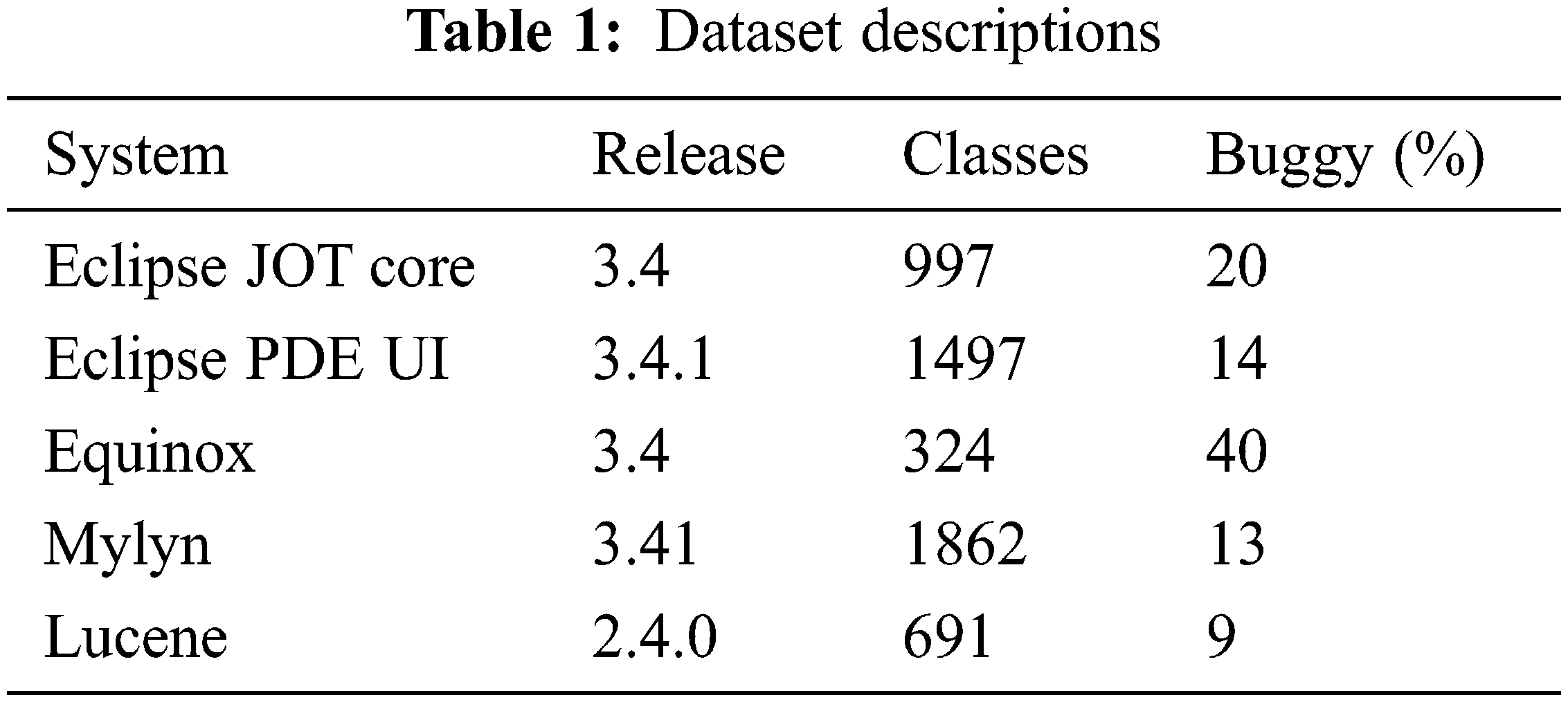
The performance validation of the MODL-SBP technique takes place using five benchmark datasets, which comprises of distinct classes [24]. The details of the dataset are given in Tab. 1. The results are inspected under two aspects such as Before Parameter Tuning (BPT) and After Parameter Tuning (APT).
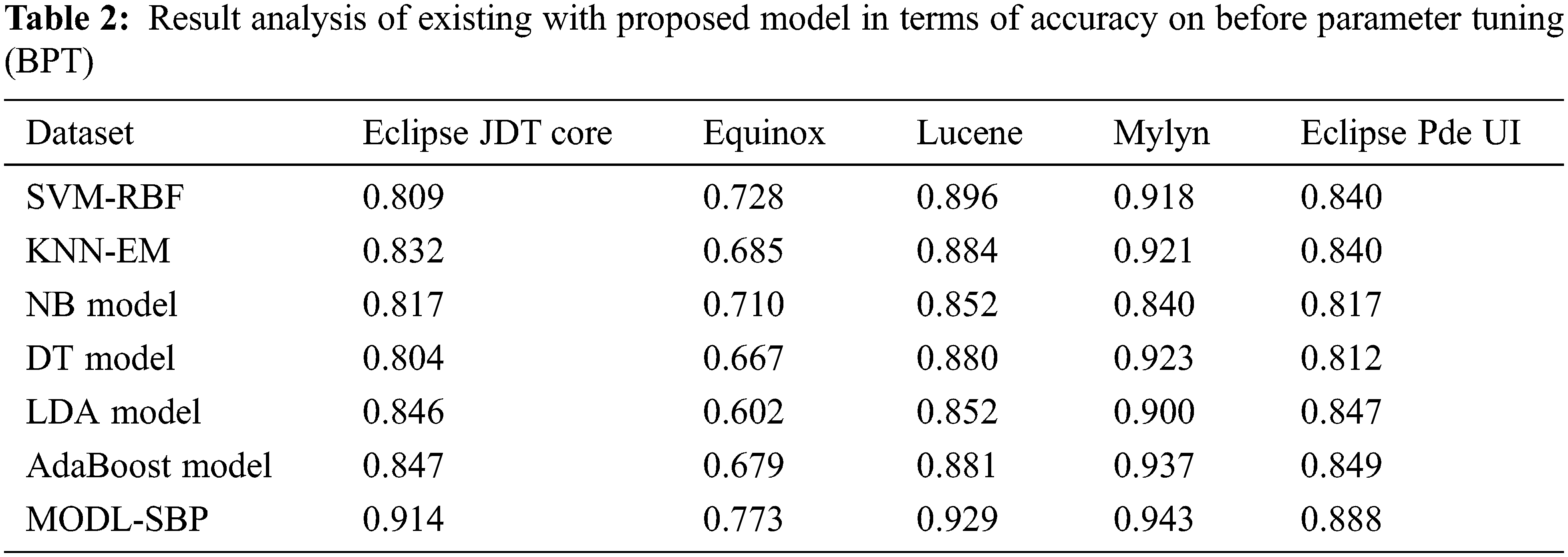
The accuracy study of the MODL-SBP technique under the BPT process is presented in Tab. 2 and Fig. 3. The results demonstrate that the MODL-SBP technique achieved the highest level of accuracy across all test datasets. For example, the MODL-SBP strategy achieved a better accuracy of 0.914 using the Eclipse JDT Core dataset, whereas the SVM-RBF, KNN-EM, NB, DT, LDA, and AdaBoost strategies achieved lesser accuracy of 0.809, 0.832, 0.817, 0.804, 0.846, and 0.847, respectively. Furthermore, using the Lucene dataset, the MODL-SBP strategy achieved the highest accuracy of 0.929, while the SVM-RBF, KNN-EM, NB, DT, LDA, and AdaBoost techniques achieved lower accuracy of 0.896, 0.884, 0.852, 0.880, 0.852, and 0.881, respectively. Furthermore, with the Eclipse Pde UI dataset, the MODL-SBP strategy achieved an accuracy of 0.888, whilst the SVM-RBF, KNN-EM, NB, DT, LDA, and AdaBoost techniques achieved an accuracy of 0.840, 0.840, 0.817, 0.812, 0.847, and 0.849, respectively.

Figure 3: Accuracy analysis of MODL-SBP technique under BPT process
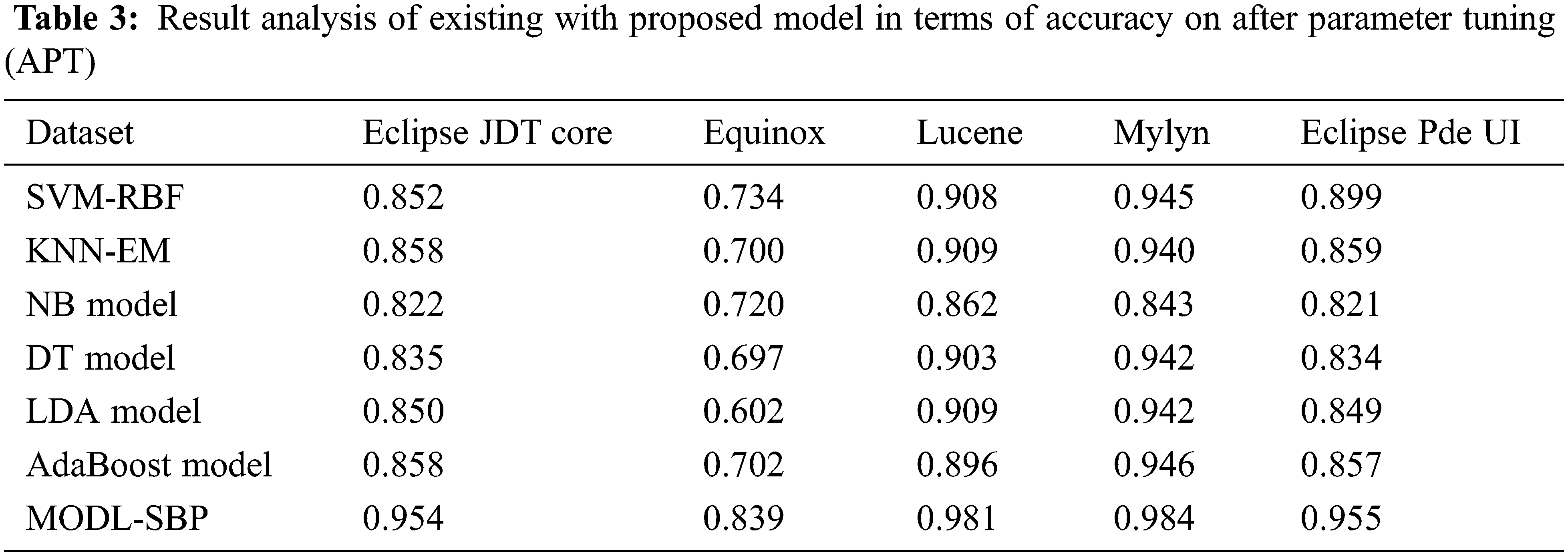
The accuracy study of the MODL-SBP algorithm under APT is presented in Tab. 3 and Fig. 4. The results show that the MODL-SBP approach achieved maximum accuracy on all test datasets. For example, the MODL-SBP approach achieved a better accuracy of 0.954 with the Eclipse JDT Core dataset, whereas the SVM-RBF, KNN-EM, NB, DT, LDA, and AdaBoost techniques achieved minimal accuracy of 0.852, 0.858, 0.822, 0.835, 0.850, and 0.858, respectively. The MODL-SBP technique achieved a maximum accuracy of 0.981 with the Lucene dataset, whereas the SVM-RBF, KNN-EM, NB, DT, LDA, and AdaBoost systems achieved minimum accuracy of 0.908, 0.909, 0.862, 0.903, 0.909, and 0.896, respectively. Finally, the MODL-SBP strategy achieved a greater accuracy of 0.955 using the Eclipse Pde UI dataset, whereas the SVM-RBF, KNN-EM, NB, DT, LDA, and AdaBoost methods achieved lesser accuracy of 0.899, 0.859, 0.821, 0.834, 0.849, and 0.857, respectively.
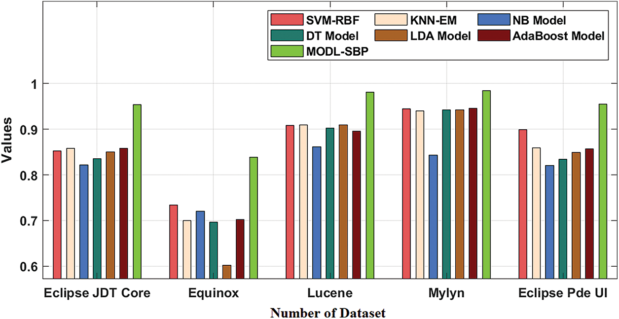
Figure 4: Accuracy analysis of MODL-SBP technique under APT process
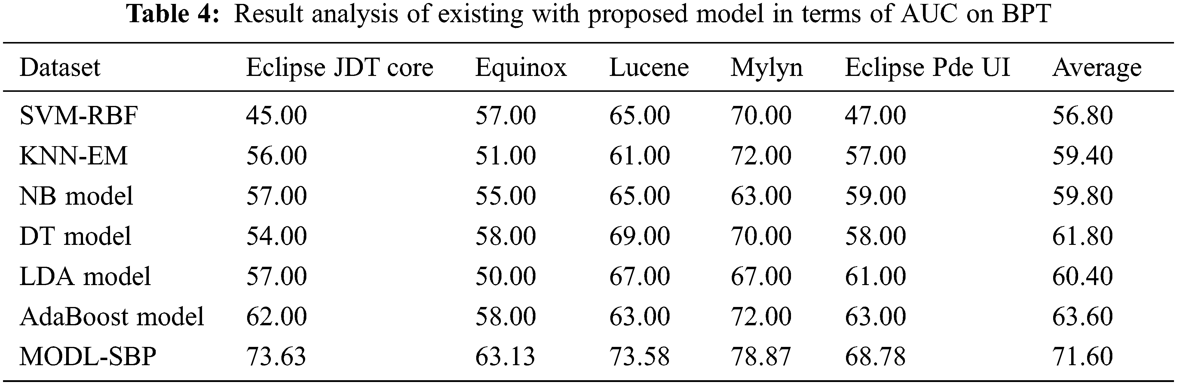
The AUC analysis of the MODL-SBP technique under the BPT process is shown in Tab. 4 and Fig. 5. The results reveal that the MODL-SBP approach achieved a higher AUC on all test datasets. For example, with the Eclipse JDT Core dataset, the MODL-SBP approach achieved a higher AUC of 73.63%, whereas the SVM-RBF, KNN-EM, NB, DT, LDA, and AdaBoost techniques achieved lesser AUCs of 45%, 56%, 57%, 54%, 57%, and 62%, respectively. Similarly, with the Lucene dataset, the MODL-SBP approach achieved the highest AUC of 73.58%, whereas the SVM-RBF, KNN-EM, NB, DT, LDA, and AdaBoost strategies had lesser AUCs of 65%, 61%, 65%, 69%, 67%, and 63%. Finally, with the Eclipse Pde UI dataset, the MODL-SBP technique has a higher AUC of 71.60%, whereas the SVM-RBF, KNN-EM, NB, DT, LDA, and AdaBoost approaches have lesser AUCs of 56.80%, 59.40%, 61.80%, 60.40%, and 63.60%, respectively.
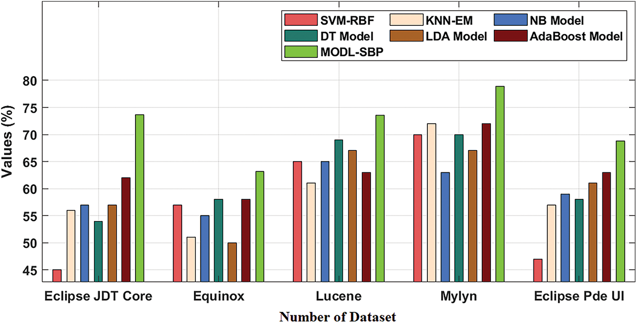
Figure 5: AUC analysis of MODL-SBP technique under BPT process
The AUC analysis of the MODL-SBP approach under APT is presented in Tab. 5 and Fig. 6. The results reveal that the MODL-SBP approach achieved a higher AUC on all test datasets. For example, with the Eclipse JDT Core dataset, the MODL-SBP methodology achieved an AUC of 90.04%, whereas the SVM-RBF, KNN-EM, NB, DT, LDA, and AdaBoost methods achieved AUCs of 86%, 80%, 68%, 70%, 65%, and 73%, respectively. Furthermore, with the Lucene dataset, the MODL-SBP technique achieved the highest AUC of 85.31%, whereas the SVM-RBF, KNN-EM, NB, DT, LDA, and AdaBoost strategies achieved lower AUCs of 78%, 71%, 68%, 77%, 80%, and 77%, respectively. Finally, with the Eclipse Pde UI dataset, the MODL-SBP technique achieved an AUC of 84.60%, while the SVM-RBF, KNN-EM, NB, DT, LDA, and AdaBoost algorithms achieved AUCs of 77.40%, 72.80%, 65.40%, 73%, 71%, and 73.80%, respectively.

Figure 6: AUC analysis of MODL-SBP technique under APT process
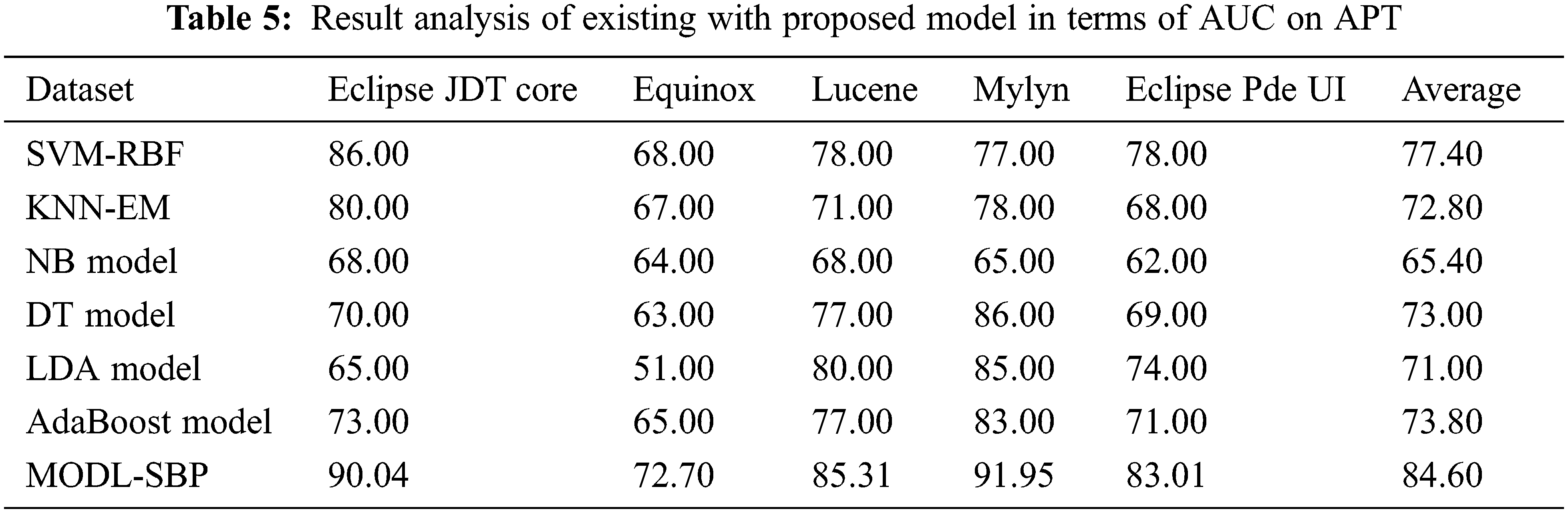
Fig. 7 offers an average accuracy and AUC analysis of the MODL-SBP technique under BPT and APT. The figures depict that the MODL-SBP technique has offered the maximum performance in terms of accuracy and AUC over the other methods compared.
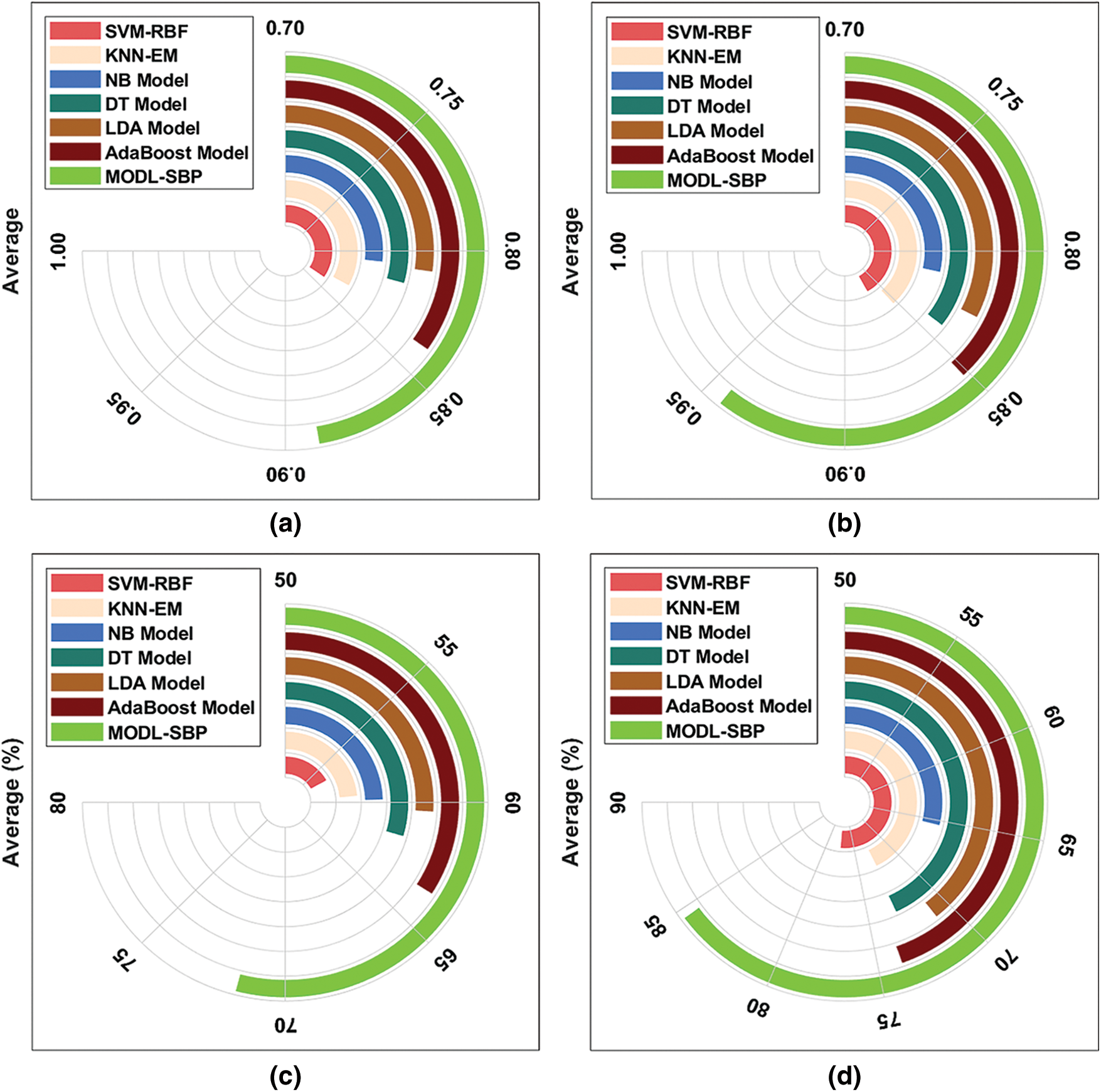
Figure 7: Average result analysis of MODL-SBP technique (a) Accuracy-BPT (b) Accuracy-APT (c) AUC-BPT (d) AUC-APT
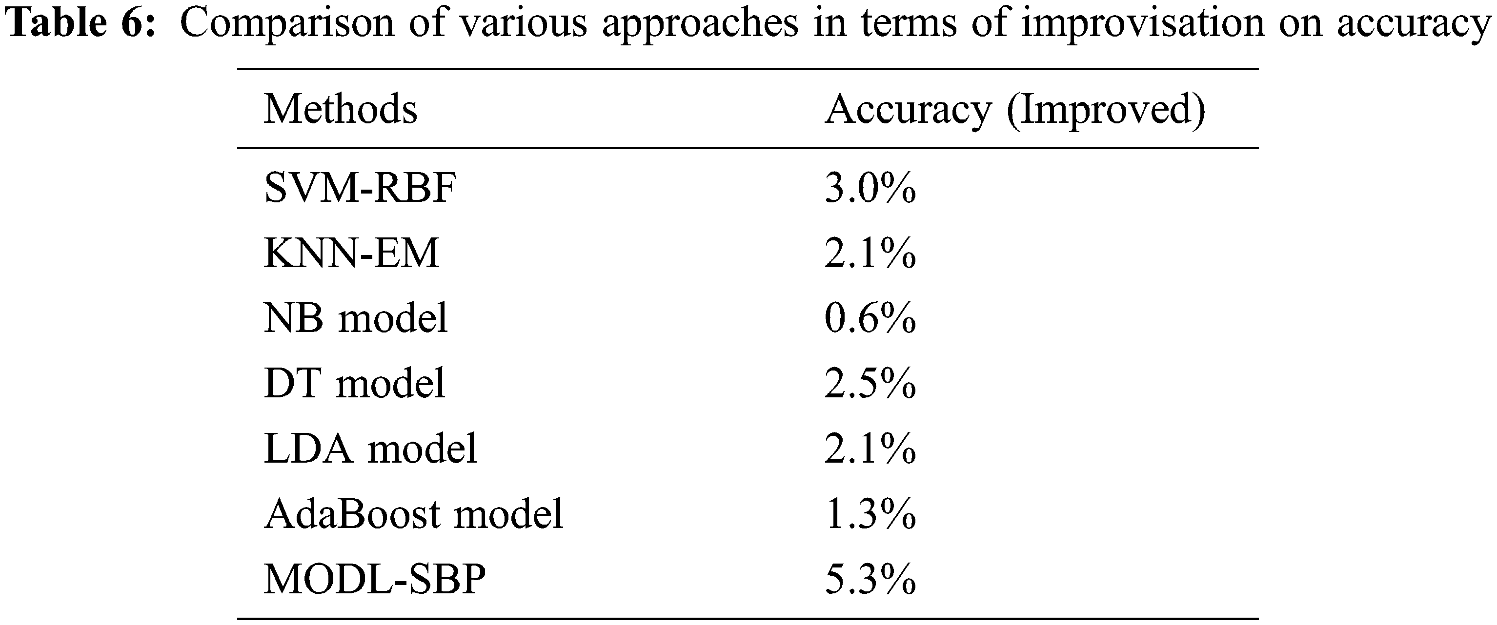
Finally, as shown in Tab. 6 and Fig. 8, a full comparative result analysis of the MODL-SBP methodology with recent methodologies is performed in terms of enhanced accuracy. The results demonstrate that the NB model performed poorly in comparison to the other strategies. Following that, the KNN-EM, DT, DA, and AdaBoost models achieved a reasonable performance. In keeping with this, the SVM-RBF approach resulted in a 3% boost in accuracy. The new MODL-SBP technique, on the other hand, surpassed the current strategies with a maximum accuracy improvement of 5.3%. The full result analysis clearly shows that the MODL-SBP technique is a useful tool for SBP.

Figure 8: Comparative analysis of MODL-SBP technique with existing approaches
A unique MODL-SBP approach was created in this work to forecast the existence of software flaws, ensuring software dependability and trustworthiness. The proposed MODL-SBP approach treats the SBP as a classification issue that is addressed using DL models. Furthermore, the MODL-SBP approach used the CNN-BiLSTM model to discover software flaws. Furthermore, CQGOA is used to tune the hyperparameters of the CNN-BiLSTM model. To investigate the improved performance of the MODL-SBP approach, a thorough experimental study is performed, and the findings are scrutinized in a variety of ways. The simulation results demonstrated that the suggested MODL-SBP method outperformed current state-of-the-art SBP techniques. In the future, hybrid metaheuristic optimization techniques may be created to successfully adjust the DL models’ hyperparameters.
Funding Statement: The authors received no specific funding for this study.
Conflicts of Interest: The authors declared that they have no conflicts of interest regarding the present study.
1. A. Hammouri, M. Hammad, M. Alnabhan and F. Alsarayrah, “Software bug prediction using machine learning approach,” International Journal of Advanced Computer Science and Applications, vol. 9, no. 2, pp. 78–83, 2018. [Google Scholar]
2. S. Divyabharathi, “Large scale optimization to minimize network traffic using MapReduce in big data applications,” in Int. Conf. on Computation of Power, Energy Information and Communication, India, pp. 193–199, 2016. [Google Scholar]
3. S. Shivaji, E. J. Whitehead, R. Akella and S. Kim, “Reducing features to improve bug prediction,” in IEEE/ACM Int. Conf. on Automated Software Engineering, Auckland, New Zealand, pp. 600–604, 2009. [Google Scholar]
4. D. Paulraj, “An automated exploring and learning model for data prediction using balanced ca-svm,” Journal of Ambient Intelligence and Humanized Computing, vol. 12, no. 5, pp. 1–15, 2020. [Google Scholar]
5. D. L. Gupta and K. Saxena, “Software bug prediction using object-oriented metrics,” Sādhanā, vol. 42, no. 5, pp. 655–669, 2017. [Google Scholar]
6. H. Osman, M. Ghafari and O. Nierstrasz, “Hyperparameter optimization to improve bug prediction accuracy,” in IEEE Workshop on Machine Learning Techniques for Software Quality Evaluation (MaLTeSQuE), Klagenfurt, Austria, pp. 33–38, 2017. [Google Scholar]
7. M. Sundaram, S. Satpathy and S. Das, “An efficient technique for cloud storage using secured de-duplication algorithm,” Journal of Intelligent & Fuzzy Systems, vol. 42, no. 2, pp. 2969–2980, 2021. [Google Scholar]
8. M. A. Berlin and S. Tripathi, “IoT-based traffic prediction and traffic signal control system for smart city,” Soft Computing, vol. 25, no. 8, pp. 12241–12248, 2021. [Google Scholar]
9. C. Ramalingam, “Addressing semantics standards for cloud portability and interoperability in multi cloud environment,” Symmetry, vol. 13, no. 2, pp. 1–12, 2021. [Google Scholar]
10. S. Sambit, S. Debbarma, S. C. Sengupta Aditya and K. D. Bhattacaryya Bidyut, “Design a fpga, fuzzy based, insolent method for prediction of multi-diseases in rural area,” Journal of Intelligent & Fuzzy Systems, vol. 37, no. 5, pp. 1064–1246, 2019. [Google Scholar]
11. A. Arun, R. R. Bhukya, B. M. Hardas and T. Ch, “An automated word embedding with parameter tuned model for web crawling,” Intelligent Automation & Soft Computing, vol. 32, no. 3, pp. 1617–1632, 2022. [Google Scholar]
12. F. Khan, S. Kanwal, S. Alamri and B. Mumtaz, “Hyper-parameter optimization of classifiers, using an artificial immune network and its application to software bug prediction,” IEEE Access, vol. 8, no. 2, pp. 20954–20964, 2020. [Google Scholar]
13. S. K. Pandey, R. B. Mishra and A. K. Tripathi, “BPDET: An effective software bug prediction model using deep representation and ensemble learning techniques,” Expert Systems with Applications, vol. 144, no. 1, pp. 113085, 2020. [Google Scholar]
14. P. V. Rajaram and P. Mohan, “Intelligent deep learning based bidirectional long short term memory model for automated reply of e-mail client prototype,” Pattern Recognition Letters, vol. 152, no. 12, pp. 340–347, 2021. [Google Scholar]
15. P. K. Chaubey and T. K. Arora, “Software bug prediction and classification by global pooling of different activation of convolution layers,” Materials Today: Proceedings, vol. 26, no. 2, pp. 154–161, 2020. [Google Scholar]
16. D. Venu, A. V. R. Mayuri, G. L. N. Murthy, N. Arulkumar and S. Nilesh, “An efficient low complexity compression based optimal homomorphic encryption for secure fiber optic communication,” Optik, vol. 252, no. 1, pp. 1–15, 2022. [Google Scholar]
17. Y. Qu, J. Chi and H. Yin, “Leveraging developer information for efficient effort-aware bug prediction,” Information and Software Technology, vol. 137, no. 2, p.1 06605, 2021. [Google Scholar]
18. C. Pretty Diana Cyril, J. Rene Beulah, P. Mohan, A. Harshavardhan, D. Sivabalaselvamani et al., “An automated learning model for sentiment analysis and data classification of twitter data using balanced CA-SVM,” Concurrent Engineering: Research and Applications, vol. 28, no. 4, pp. 386–395, 2021. [Google Scholar]
19. Y. Qu and H. Yin, “Evaluating network embedding techniques’ performances in software bug prediction,” Empirical Software Engineering, vol. 26, no. 4, pp. 1–44, 2021. [Google Scholar]
20. N. Subramanian and D. Paulraj, “A gradient boosted decision tree-based sentiment classification of twitter data,” International Journal of Wavelets, Multiresolution and Information Processing, vol. 18, no. 4, pp. 1–21, 2020. [Google Scholar]
21. C. Saravanakumar, R. Priscilla, B. Prabha, A. Kavitha and C. Arun, “An efficient on-demand virtual machine migration in cloud using common deployment model,” Computer Systems Science and Engineering, vol. 42, no. 1, pp. 245–256, 2022. [Google Scholar]
22. S. Z. Mirjalili, S. Mirjalili, S. Saremi, H. Faris and I. Aljarah, “Grasshopper optimization algorithm for multi-objective optimization problems,” Applied Intelligence, vol. 48, no. 4, pp. 805–820, 2018. [Google Scholar]
23. C. Ramalingam and P. Mohan, “An efficient applications cloud interoperability framework usingi-anfis,” Symmetry, vol. 13, no. 2, pp. 1–15, 2021. [Google Scholar]
24. H. B. Duan, C. F. Xu and Z. H. Xing, “A hybrid artificial bee colony optimization and quantum evolutionary algorithm for continuous optimization problems,” International Journal of Neural Systems, vol. 20, no. 01, pp. 39–50, 2010. [Google Scholar]
 | This work is licensed under a Creative Commons Attribution 4.0 International License, which permits unrestricted use, distribution, and reproduction in any medium, provided the original work is properly cited. |