DOI:10.32604/iasc.2022.024998
| Intelligent Automation & Soft Computing DOI:10.32604/iasc.2022.024998 | |
| Article |
Anatomical Region Detection Scheme Using Deep Learning Model in Video Capsule Endoscope
1Department of Information Technology, National Engineering College, Kovilpatti, 628503, Tamilnadu, India
2Department of Electronics and Instrumentation Engg., National Engineering College, Kovilpatti, 628503, Tamilnadu, India
3Department of Electronics and Communication Engg., Ramco Institute of Technology, Rajapalayam, 626117, Tamilnadu, India
*Corresponding Author: S. Rajagopal. Email: rajatarget@nec.edu.in
Received: 07 November 2021; Accepted: 19 January 2022
Abstract: Video capsule endoscope (VCE) is a developing methodology, which permits analysis of the full gastrointestinal (GI) tract with minimum intrusion. Although VCE permits for profound analysis, evaluating and analyzing for long hours of images is tiresome and cost-inefficient. To achieve automatic VCE-dependent GI disease detection, identifying the anatomical region shall permit for a more concentrated examination and abnormality identification in each area of the GI tract. Hence we proposed a hybrid (Long-short term memory-Visual Geometry Group network) LSTM-VGGNET based classification for the identification of the anatomical area inside the gastrointestinal tract caught by VCE images. The video input data is converted to frames such that the converted frame images are taken and are processed. The processing and classification of health condition data are done by the use of Artificial intelligence (AI) techniques. In this paper, we proposed a prediction of medical abnormality from medical video data that includes the following stages as given: Pre-processing stage performs using Gabor filtering, histogram-based enhancement technique is employed for the enhancement of the image. Multi-linear component analysis-based feature selection is employed, and the classification stage performs using Hybrid LSTM-VGGNET with the performance of accurate prediction rate.
Keywords: Video capsule endoscope (VCE); gabor filtering; semantic entropy-based feature extraction; hybrid LSTM-VGGNET
Video capsule endoscope (VCE) is regarded as the most emergent means of technology for allowing entire gastrointestinal tract examination with negligible invasion. Many indirect procedures like angiography, echo sounding, x-radiography (including CT), and dispensing to identify diseases of the GI tract have been established. Unfortunately, they have been found to have little diagnostic efficiency or are occasionally beneficial even in bleeding detection until they are very active. The greatest way to discover and detect GI problems is by physically examining the GI tract, making endoscopy a direct and effective diagnostic technique. The whole stomach, intestine, and colon may be viewed in a wired endoscopic inventory [1]. As endoscopy, since the clinic has the opportunity to see the GI tract directly, is the usual methodology and criterion to diagnose GI disease [2]. The standard wired invasive endoscopy, however, is physically constrained and the entire GI system cannot be examined [3]. They are uncomfortable and give patients severe discomfort. There might be an increased risk of bowel perforation and cross-contamination. The diagnosis of the underlying cause of GI bleeding typically begins with the doctor inquiring about your health history and symptoms [4]. A stool sample may also be requested from the doctor to check for evidence of anemia, along with another testing. Upper GI bleeding is identified most often when an endoscopic test is performed. The fast frame rate and high-resolution photographs are one of the trends in this new technology [5]. The live GI organ is always moving; hence the 2-section frame rate is not sufficient to diagnose GI organ features. WCE’s optimal frame rate is the same as the WCE video. Now some WCE video systems were created, and in NTSC video format, the CE may send GI tract pictures with a frame rate of 30 f/s. On the second side, the picture resolution of 256 × 256 in comparison to wired endoscopy is not satisfied and the picture resolution is no longer too high. However, the high frame rate and the excellent image quality are attained. For a higher frame rate, the video compression techniques will be helpful. The video files are transmitted over the communication network as a part of data sharing. To achieve fast data transfer, the video file is compressed. The transmission network contains noise parameters in various forms. The compressed data gets deteriorated due to induction of noise and some packets are lost. The traditional method of data rectification like Error Correction Code (ECC) was used to reduce packet loss at the receiving end. The Cyclic Redundancy Check (CRC) method was executed at the receiving end to correct the error bit. This method is highly complex and consumes more time. The previous ECC algorithm will block any erroneous data and the transmitter has to resend the entire data. The transmission channel contains noises. This noise will deviate from the properties of the transmitted data. Also, the deep learning methods for the detection of various anatomical areas in an effective manner in the entire VCE image sequence not only save time thereby focusing and directing various regions assessment for the automatic eventual VCE dependent disease detection. The detection of anatomical areas in VCE images instinctively means identifying developed features of semantic images that differentiate one region of the GI tract from others. In this article, a deep learning-dependent design is investigated for the identification of anatomical regions in the images of VCE.
The further portion of the article is systematized as shown: Section 2 is the depiction of different existing methods used so far. Section 3 is the detailed explanation of the suggested strategy. The behavioral analysis of the suggested technique is shown in Section 4. Finally, the overall flow of the proposed system is deduced in Section 5.
The author in paper [6] have used a histogram of the highest block value extricated from a level of Red-Green intensity value as discriminating features for preparing a KNN classifier for identification of bleeding. In [7] a SVM classifier prepared with 5 color characteristics was proposed that attains an accuracy of detection of 97.5% with an RBF kernel. The authors have lengthened the study in [8] with color, structure, and combined color and structure characteristics. Three diverse classifiers dependent on Random Forest, Logistic Model Tree, and Random Tree are prepared with a collection of five color characteristics, five perfect structure characteristics, and three mixtures of structure and color characteristics. The structure characteristics in each feature collection are chosen from an entire collection of twenty two GLCM characteristics. [9] introduced a bleeding identification approach with histogram feature extricated from the region of interest segmented from the standardized Red Green Blue color area. A two-step independent bleeding identification method depending on color enhancement is provided in [10]. This article uses the retinex hypothesis of color recognition for color improvement in the initial step and pertinent area identification in the next. It is proved that anomaly identification maximizes with color improvement.
An optimal FEC process to identify the ideal and channel coding rate to transfer video packets with minimum loss in a noise-prone network is proposed by [11]. The maximum video quality was maintained by adjusting the coding rate in the channel loss. The threshold is set in the presence of all disturbing channel conditions. The analytical method to model FEC code rate decision schemes was complex and costly. Hence a joint model in a simple closed-form was proposed by [12]. It contained a minimum count of scene-based specifications. This method estimated the optimal FEC Code rate with less computation difficulty. Wireless video streaming was a challenging task with varying video quality in the network due to changes in the network parameters. Various adaptations were made at transmitting and receiving ends to compensate for loss and to maintain video quality [13]. Proposed standardized scalable video coding technique with iterative steps to allot bitrates for various incoming video streams. It maximizes the weighted total of video features related to various streams. The work lacked spatial scalability. [14] introduced an optimized method for Bit-level IL-FEC coded expandable video transfer over the wireless network. The PSNR value was increased than the conventional UEP methods. The algorithm had to accompany enhanced FEC codes like LDPC, BICM, and TCM, etc. Ttransmitting un-coded video over a wireless communication network was a challenging task. Most data were lost in the transmission system. Hence improvement in the transmission efficiency is necessary. The system of managing garbage and the ability to gather the trash currently don’t fit the present condition. [15] stated the conventional machine and deep learning methods to validate the brain tumors. The brain tumor identification, segmentation, and categorization are efficiently made with the three unique algorithms to attain better performance employing Deep Learning (DL) methods. The accuracy and robustness of the proposed method provide better performance. [16] projected the brain tumor diagnosis of a high-end system using ‘Data, Image segmentation processing, and View’ (DIV). According to the Deep Learning (DL) neural networks, the completeness and acceptance perform in the DIV taxonomy evaluated. The prone error and time consumption are the crucial factors here, which are attained better over the existing segmentation approaches. [17] planned the Brain Tumor Segmentation Challenge (BraTS) of ensemble learning methods. To enable the reliable automatic segmentation and decision support algorithms help to a strong development of brain tumor detection and intensification MRI by the concern of segmentation algorithms. The accuracy, precision, and efficiency with better performance of brain tumor detection. [18] wished-for the segmentation of brain tumors through the association of CRF with Deep Medic or Ensemble and Conditional Random Field with fully convolutional neural network for efficient brain tumor segmentation utilizing the MRI brain image with start-of-art of quantitative analysis. [19] allowed the improved brain tumor detection method for malignancy brain tumor identification. The detection of lesions is a challenging task due to inadequate soft-tissue contrast, which enabled the lack of accurate prediction and the need to attain a better segmentation technique utilizing adaptive k-means clustering. The segmented images get classified through the Support Vector Machine classifier based on the image intensity, shape, and region of interest. [20] presented the time cycle-WCE, an end-to-end enrollment of automated method of regions of interest on WCE images. The analysts will be capable of determining the ROI employing attaining bounding boxes in some WCE frames that were to be enrolled. The presented technique depends on the model of deep learning for time-stability in the periodic enrolling scheme and the cycle of self-registering which is unsupervised entirely without any labels.
Though a substantial number of efforts were taken for minimizing the time consumption for analyzing the VCE images, minimized rate of attention were paid for developing the models which differentiate various regions of the GI tract automatically. The traditional techniques only focus on minimum-level extrication of features joined with dimensionality minimization for solving the issues of anatomical area segmentation in the GI tracts. Explicitly, [21] employed an analysis of color change patterns for segmenting video into anatomic parts.
This part is a detailed illustration of the suggested system explanation. The video capsule endoscope is processed to detect and classify anatomical regions. The classification process is carried out employing deep learning techniques. The entire flow of the suggested technique is shown in Fig. 1.

Figure 1: Flow of the proposed system
3.1 Input Dataset Preprocessing & Segmentation
After the collection of the dataset, the input video capsule endoscopy dataset is converted to frames. The input multiple frames are then preprocessed by taking the images of frames. Preprocessing is an important part to indicate the anatomical regions. Preprocessing is to confirm the reliability and accessibility of this database. Each step is important to reduce the image processing workload. Using filtering and extraction methods, preprocessing is done to detect unintended defects that can affect the region’s ability to foresee the illness. In the first case, all VCE images are updated to include those pixels based on the deep models applied to the different datasets. Pre-processing is done using filters and histogram equalization techniques to detect unintentional errors that can impair the ability of the artifact to prevent disease. Here we can extract an abnormality in the area from the VCE image. A non-linear optical filtering system called an adaptive median filter is occasionally utilized to eliminate noise from an image or signal. The main advantage of removing noise reduction is an archetypal preprocessing step for better performance. In general, the VCE image comprises three (red, green, blue) channels. The blue channel loses its greatest clarity and contrasts sharply. Second, during preprocessing it blocks the green channel. Typically, poor contrast occurs with x-ray objects. Preprocessing is achieved to increase the green channel’s contrast. Typically, histogram equalization is done to the improvement of image quality. Histogram Equalization is a method used to escalation the contrast of images. It is achieved by effectively growing the most normal intensity values, i.e., by expanding the picture intensity range. The distinction between areas is rendered fewer local in contrast. Thus, the average image contrasts are increased by following the histogram equalization, which is a process that requires intensity adjustment, thus increasing contrast, indicated by P as the uniform histogram of an image for each possible intensity.
This method can be used for improving image quality with histogram equalization. Then, by changing the RGB values, the sensitivity may then be calibrated.
Gabor filtering is the lead role in the VCE images, which was to improve the contrast. Gabor filters were used for the identification of structures and boundaries of the GI tract in VCE images. The thresholding approach in an extraction mask is produced and utilized the boundaries and connectivity through their respective threshold value. For further enhancement work, the Gabor filter is applied to enumerate the VCE images. Gabor filter responds to the healthy and unhealthy of the sampled images of VCE. The training of datasets is remodeled according to their respective intensity features. The remodeled attributes as well as conventional segmented images. For fundus photograph evaluation, the Gabor filters are more effective. Moreover, Gabor filtering is used to enhance the given datasets of the VCE images. The following steps are used to improve the VCE images at some irregularities of noise.
3.2 Segmentation Process Using Watershed Approach
This is the next stage of preprocessing that enhanced the features of the thresholding VCE images. By using this method, constructing the given threshold values among the given regions from their boundaries of the segmented level of features. Watershed segmentation is used for the best multiresolution of VCE images. Although the watershed segmentation is very useful in a certain degree of VCE images. The noise in the VCE images on the grayscale image, which carries the capturing process by using the watershed segmentation algorithm, can be reduced. The low-resolution image can be segmented through the use of a watershed segmentation algorithm, which was extracted from the thresholding images. The process undertaken the low pass filtered fundus images through the exemption of noise from the given images.
3.3 Semantic Entropy-Based Feature Extraction and Multi-Linear Component Analysis-Based Feature Selection Approach
Semantic entropy-based extraction is carried out. Bi-level image thresholding in which the image can be split between the target and the background in two sections. The threshold at the two-level is not very efficient if the image is a complex one involving several artifacts. In such a scenario, multi-level thresholding is often used to segment an image. Nevertheless, the appropriate values of such thresholds must be chosen to achieve efficient segmentation. Optimal selection thresholding approaches pursue thresholds by modifying undefined functions (whether they will be decreased or increased). The Masi entropy of class variance approaches is the most widely employed optimum thresholding strategy. In the following paragraphs, we make a brief statement of the above entropy. Suppose that Ithnumbers of grey rates are in the range in a specific image {0, 1, 2,…(Ith −1). Let N be the total pixel count in the image. In the image, a particular gray level j happens nj times. The gray histogram of the image may be translated and being used as a collection of possibilities. The probability of a gray level is established by j as Pj = nj/N. The following subsections describe Masi entropy between class variance functions in an elaborated way. Masi approach chooses the optimal levels by increasing the entropy of the segmented groups. Masi method defines the entropy of an image assuming its gray-level histogram entirely represents an image. If m numbers of thresholds are to be chosen [h1, h2,…, hm] which divides up the image into groups (c0, c1,….cn) then Masi does so by optimizing the objective function.
where
Here
Multi-linear Component Analysis for Feature Selection
The functionality can then be removed and the extracted features were selected using the Multi-linear Component Analysis process. This is a way to delete mathematical aspects of the second degree. In many applications, this method has been used. This is a math task that usually efficiently removes the errors. It can also be made clear how accurate the data is. During the analysis cycle, the data can be differentiated. Multi-linear Component Analysis may determine the frequency of the data in a particular exact differential field. There is a question about the single data and information is termed as the Ø route l and the adjoining value separation m. In general, m gets a single value and Ø is directionally advantageous. Then the attained directional value shall eliminate the aspects of the data. The feature extraction procedure shall be set as shown:
In which G denotes frequency vector, m, n, o denotes the frequency of the specific element that usually has the values of l and m, K denotes the characteristics of the data, (m, n) was the element of m and l,
By using the Multi-linear Component Analysis approach, the different attributes can be obtained. This method also allows you to view the features. This is one of the most frequently used extraction methods. In extracting the axis from data, it shows the highest volatility. This Multi-linear Component Analysis system of assessment decides whether or not the accuracy of the data is advantageous. The criterion value of the size used by certain correlation parameters is based on the absolute and partial combination of the target and unnecessary data. The main use of Multi-linear Component Analysis is the input of regulated and unregulated classification applications to evaluate their functionality. The entire method depends on the load and input changes and IDS performance of the device. Using the function extraction method to generate the updated items throughout the selection period. Required information is removed. After that, we will remove some of the essential features below. The length and characteristics of the information are defined as follows:
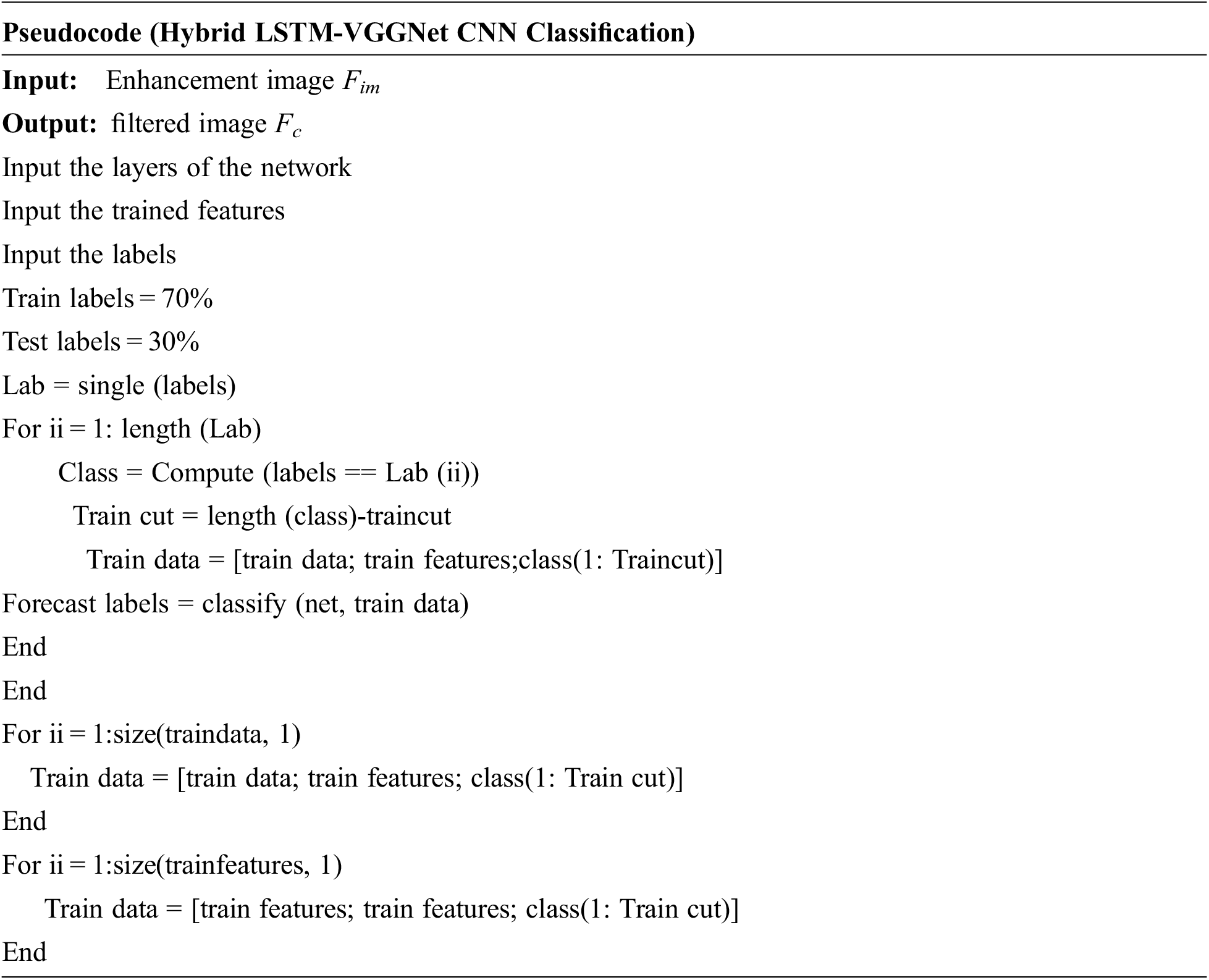
3.4 Hybrid LSTM-VGGnet Classification to Detect Anatomical Regions
There are 24 convolutional layers and two fully connected layers available in the framework of this design. The convolution layer sex tricate the characteristics whereas the fully connected layers evaluate the position and possibilities of the boundary strata. Initially, we split the full image into a panel grid of measurement n × n. Every grid cell relates with two bounding boxes and corresponding category determinations, thus we shall detect a maximum of two items in a single grid cell. When an item covers over one grid cell, we select the center cell as the point of a forecast for that item. The bounding box with no items has zero determination value whereas a bounding box close to an item possesses a determination value appropriate to the bounding box scores.
The Correlation aware LSTM based VGGNet classification can be suggested for anatomical region classification. Here in this process, the image can be identified and it can be tracked depend upon its posing. The transition into a sub-set involves an affinity. The shear transformation is not considered since shear is negligible. Thus, the transformation becomes,
If an image has been submitted, we generate multiple sub-images for each image in the database with the same number of images as the query. The images and databases are numbered with 1, 2,…, and so on to the right. Then the imaging in which the region can be identified, and the Euclidean distance can be calculated.
Finally, a ranking is generated for the abnormality matching distance of data base images,
Following the extraction of features, the bleeding region must be distinguished to decide if the diabetic is in the mild, moderate, or extreme stage [22]. For this classification, a VGG-16-based CNN, which is a well-known algorithm, was used. Probabilities are used to score the goal. It is a pre-trained convolution algorithm. Variations between a single dependent variable and one or more independent variables may be analyzed using VGG-16-based CNN. The CNN uses a function to predict probabilities. The distribution is complete. During this method, CNN will first read and resize the image before beginning the classification process by measuring the likelihood of its class. Most of the deep learning neural networks are convolution neural networks based on the VGG-16 CNN marks a major development in visual detection and classification. They are most widely used to deconstruct visual symbolism and are also used in image description and classification. A VGG-16 based CNN is stacked in the pattern of the layers.
• ReLU layer
• Convolutional layer
• Pooling layer
• Fully connected layer
When opposed to alternate image classification algorithms, VGG-16-based CNN needs the least amount of pre-processing. This CNN could be employed in a variety of areas for a variety of reasons.
(i) Convolution
This convolution step’s primary function is to focus highlights from the information frame. In VGG-16-based CNN, the convolutional layer is often the first phase. The features in the input image were identified and a feature map was generated during this process.
(ii) ReLU layer
The convolution layer is succeeded by the redressed straight unit layer. The simulation operation was used on the feature maps to increase the network’s non-linearity. Negative values can be easily omitted in this case.
(iii) Pooling:
The pooling mechanism will eventually reduce the size of the input. Over fitting can be reduced by using the pooling step. By reducing the number of necessary parameters, will easily figure out the required parameters.
(iv) Flattening
The polled function map must be flattened to a sequential column of numbers, which is a relatively easy measure.
(v) Fully Connected Layer
The functionality that can be paired with the attributes is listed here. This has the potential to finish the classification procedure with higher accuracy. The error will primarily be measured and propagated backward.
(vi) SoftMax:
SoftMax is frequently employed in neural networks, to map the non-standardized result of a network to probability dispersion over forecasted result class. The SoftMax was executed in several investigation fields for many issues. Such decimal probabilities should mean 1.0. Assume the following types of SoftMax:
• Full SoftMax that can evaluate a probability for each probable class.
• SoftMax evaluates a probability for every positive name anyhow just for a random instance of negative names.
This CNN makes it possible to measure a discrepancy between one or more of the various variables. CNN measures the chances and the work. It is what has been accrued. In this method, CNN will first interpret, redistribute, and then calculate the class likelihood of the image.
In which F denotes the feature, q represents the pointed feature, β1β2 denotes the classified features. These are to be expressed as
The CNN classification was deduced as
where V is the empirical constant.
Thus, the classification process is capable of detecting the anatomical regions from VCE images in an accurate manner. The use of our suggested method enhances the accuracy of the classifier and in turn, offers an improved outcome rate.
This part is the detailed deliberation of performance analysis of the suggested system. The dataset details are provided below. The performance outcomes estimated are compared with existing techniques to prove the effectiveness of the proposed scheme. The performance metrics employed is specified as follows:
The Accuracy Ai depends on the number of targets that are classified correctly and is evaluated by the formula
Sensitivity measures how much number of positives that are correctly identified as positives and is defined as
Precision is defined as the ratio of number targets that are classified to the number of targets present in an image.
where FN-False Negative, FP-False Positivewhere TN-True Negative, TP-True Positive,
F-measure is obtained by combining precision and recall.
4.5 Preparation of Dataset, Annotation and the Process of Augmentation
The dataset taken comprises about 9 patient’s videos or about 200,000 capsule endoscopy frames approximately. The dataset is divided depending on the anatomical areas like esophagus, small bowel, stomach, and colon. These videos were then processed into frames and were annotated by the clinical investigation professionals for identifying the various anatomical areas of the GI tract. The capsule in turn spends a varied rate of time in various regions of the GI tract, thus results in noteworthy variations in the frame numbers that were captured in each region. Thus, this causes a significant imbalance of class with greater than 80% of video capturing images of small-bowel only. The class imbalance issue was addressed by employing an up-sampling process from other areas like the stomach, colon, and esophagus for balancing the distribution of class. The images are rotated randomly to capture images for generating examples set of other regions. This experiment’s focus is to contrast the outcome attained in each area over four frameworks and not to compare the outcome of a single design over four areas of the GI tract. Hence, the procedure of augmentation was carried out only on the training set for balancing the classes whereas, the test set was left untouched.
4.6 Performance Analysis of Proposed System
The Fig. 2 provided below shows the input image dataset and the processed image outcome attained for various GI tract regions.

Figure 2: Input image and the processed outcome of various GI tract regions like (a) esophagus, (b) stomach, (c) small bowel and (d) colon
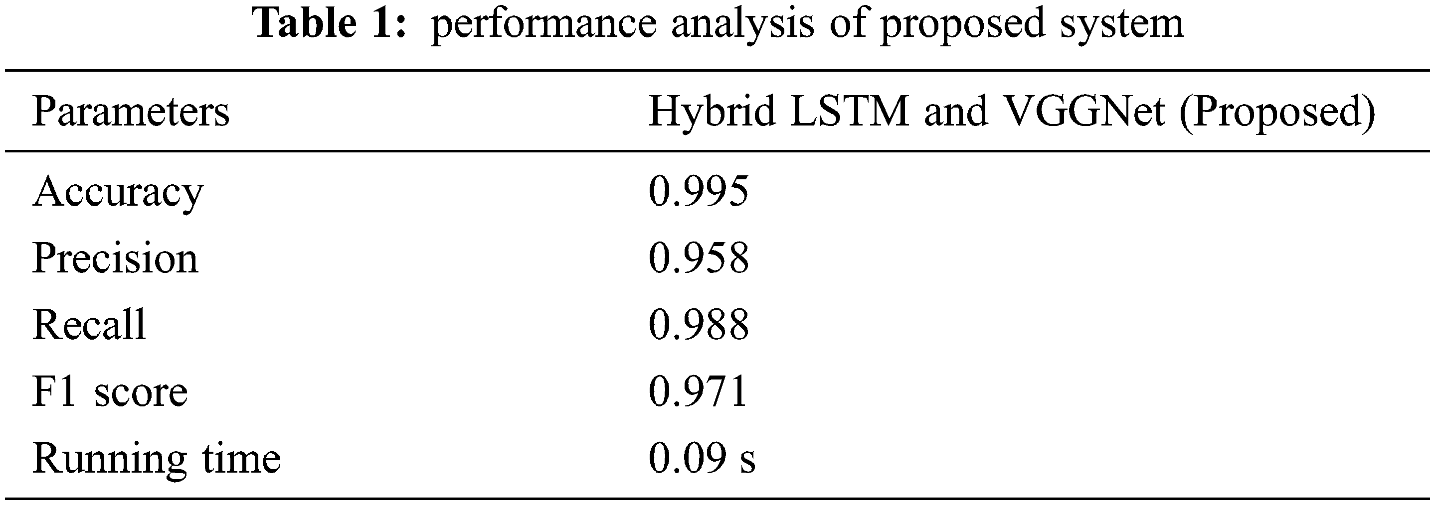
The behavioral analysis of the suggested classifier method is tabulated in Tab. 1.
4.7 Comparative Analysis of Proposed and Existing System
The proposed system performance estimated is then compared with existing techniques to prove the effectiveness of the proposed strategy. The comparisons made are shown below in graphical representations from Figs. 3–8.
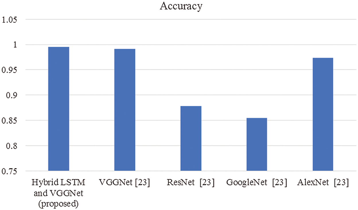
Figure 3: Comparison of accuracy
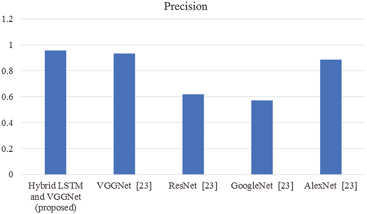
Figure 4: Comparison of precision
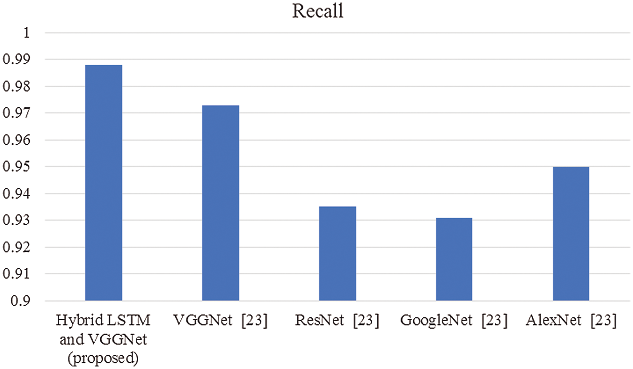
Figure 5: Comparison of recall
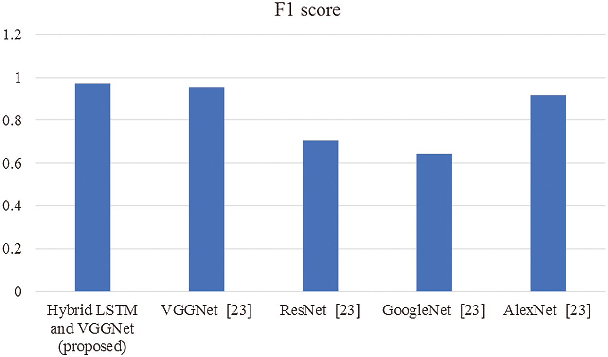
Figure 6: Comparison of F1-score
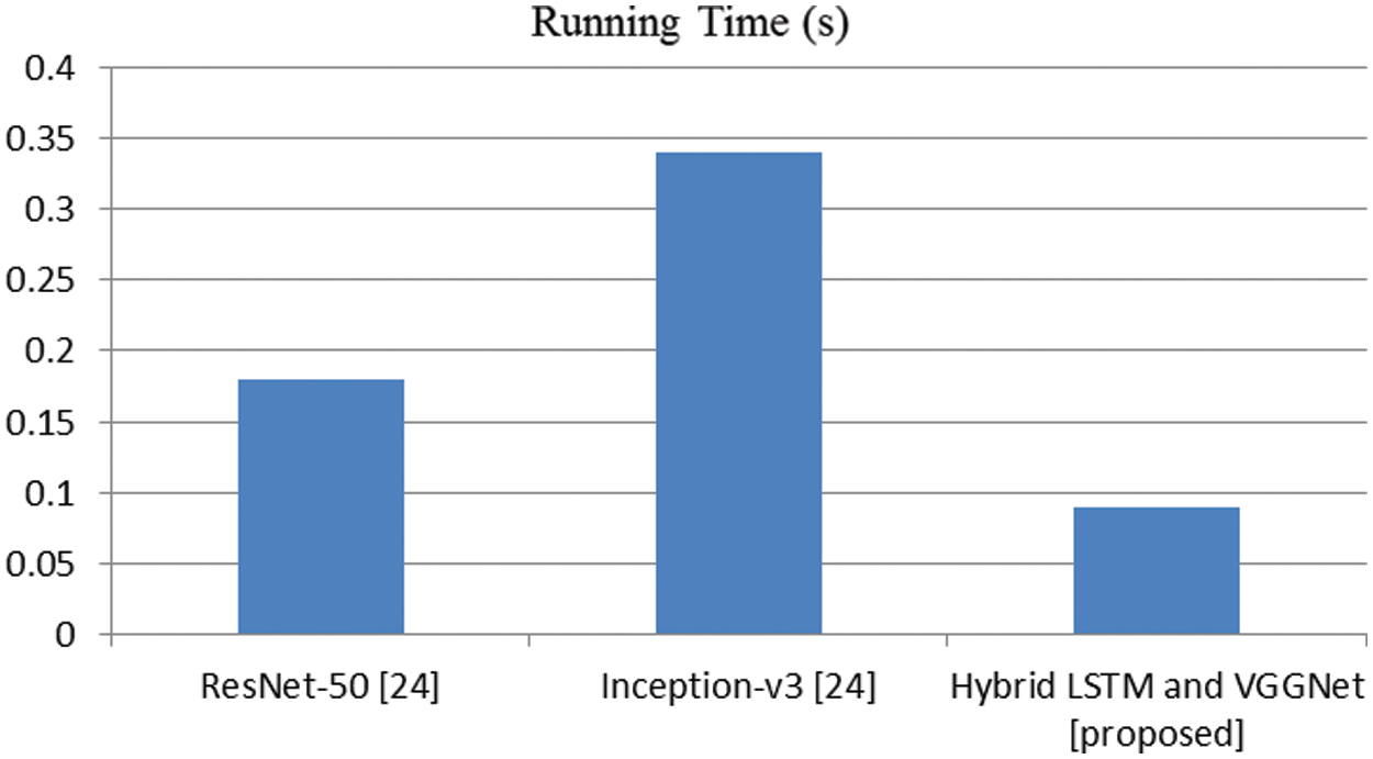
Figure 7: Comparison of running time (s)
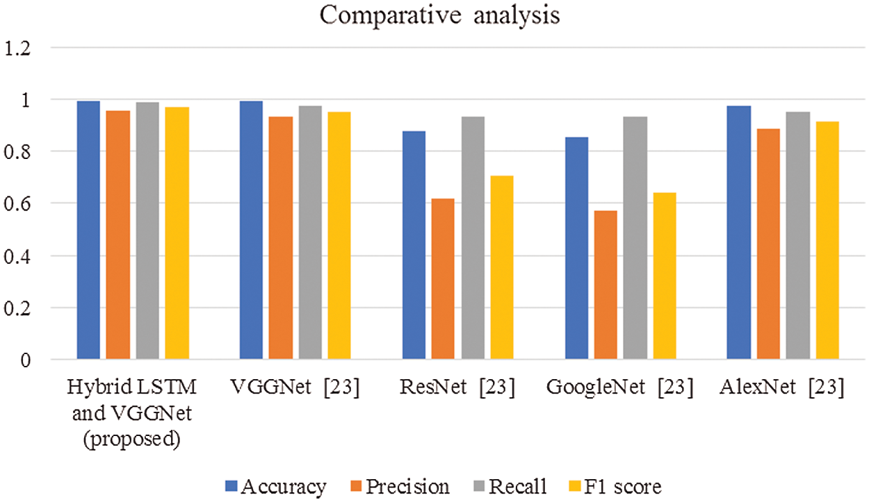
Figure 8: Overall comparisons of proposed and existing techniques
In this article, we have explained the behavior of our proposed method for the realization of anatomical elements inside the gastrointestinal tract utilizing VCE images. Empirical outcomes reveal that the proposed method could study more discriminating characteristics for identifying various regions of the gastrointestinal tract contrasted to other traditional frameworks. The proposed hybrid LSTM-VGGNet method possessed a classification accuracy of 99.5%. The performance of our suggested technique was contrasted with other existing methods. The results reveal that the suggested method surpasses the existing techniques in terms of accuracy, precision, recall, F1-score, and running time.
Funding Statement: The authors received no specific funding for this research work.
Conflicts of Interest: The authors declare that there is no conflict of interest.
1. S. Adewole, P. Fernandez, M. Yeghyayan, J. Jablonski, A. Copland et al., “Lesion2vec: Deep metric learning for few shots multiple abnormality recognition in wireless capsule endoscopy video,” in Proc. Computer Vision and Pattern Recognition, Ithaca, United States, 2021 [Online]. Available: https://arxiv.org/abs/2101.04240. [Google Scholar]
2. M. J. M. Saraiva, J. Ferreira, H. Cardoso, J. Afonso, T. Ribeiro et al., “Performance of a deep learning system for automatic diagnosis of protruding lesions in colon capsule endoscopy: A multicentric study,” 2021 [Online]. Available: https://doi.org/10.21203/rs.3.rs-284396/v1. [Google Scholar]
3. H. W. Jang, C. N. Lim, Y. S. Park, G. J. Lee and J. W. Lee, “Estimating gastrointestinal transition location using CNN-based gastrointestinal landmark classifier,” KIPS Transactions on Software and Data Engineering, vol. 9, pp. 101–108, 2020. [Google Scholar]
4. T. Aoki, A. Yamada, K. Aoyama, H. Saito, G. Fujisawa et al., “Clinical usefulness of a deep learning-based system as the first screening on small-bowel capsule endoscopy reading,” Digestive Endoscopy, vol. 32, pp. 585–591, 2020. [Google Scholar]
5. Y. Gao, W. Lu, X. Si and Y. Lan, “Deep model-based semi-supervised learning way for outlier detection in wireless capsule endoscopy images,” IEEE Access, vol. 8, pp. 81621–81632, 2020. [Google Scholar]
6. T. Ghosh, S. Fattah, C. Shahnaz, A. Kundu and M. Rizve, “Block-based histogram feature extraction method for bleeding detection in wireless capsule endoscopy,” in TENCON 2015-2015 IEEE Region 10 Conf., pp. 1–4, 2015. [Google Scholar]
7. S. Suman, F. A. B. Hussin, A. S. Malik, K. Pogorelov, M. Riegler et al., “Detection and classification of bleeding region in WCE images using a color feature,” in Proc. of the 15th Int. Workshop on Content-Based Multimedia Indexing, Florence, Italy, pp. 1–6, 2017. [Google Scholar]
8. K. Pogorelov, S. Suman, F. Azmadi Hussin, A. Saeed Malik, O. Ostroukhova et al., “Bleeding detection in wireless capsule endoscopy videos—Color versus texture features,” Journal of Applied Clinical Medical Physics, vol. 20, pp. 141–154, 2019. [Google Scholar]
9. A. K. Kundu, S. A. Fattah and M. N. Rizve, “An automatic bleeding frame and region detection scheme for wireless capsule endoscopy videos based on interplane intensity variation profile in normalized RGB color space,” Journal of Healthcare Engineering, vol. 2018, 2018. [Google Scholar]
10. F. Deeba, S. K. Mohammed, F. M. Bui and K. A. Wahid, “Unsupervised abnormality detection using saliency and retinex based color enhancement,” in 2016 38th Annual Int. Conf. of the IEEE Engineering in Medicine and Biology Society (EMBC), Orlando, FL, USA, pp. 3871–3874, 2016. [Google Scholar]
11. T. J. Jung, K. D. Seo and Y. W. Jeong, “Joint source-channel distortion model for optimal FEC code rate decision,” in Proc. Int. Conf. on Information Networking (ICOIN), Thailand, pp. 527–529, 2014. [Google Scholar]
12. T. J. Jung, K. D. Seo, Y. W. Jeong and C. K. Kim, “A practical FEC code rate decision scheme based on joint source-channel distortion model,” in Proc. IEEE Int. Symp. on Circuits and Systems (ISCAS), Melbourne, pp. 554–557, 2014. [Google Scholar]
13. H. Hu, X. Zhu, Y. Wang, R. Pan, J. Zhu et al., “Proxy-based multi-stream scalable video adaptation over wireless networks using subjective quality and rate models,” IEEE Transactions on Multimedia, vol. 15, pp. 1638–1652, 2013. [Google Scholar]
14. Y. Huo, M. El-Hajjar, R. G. Maunder and L. Hanzo, “Layered wireless video relying on minimum-distortion inter-layer FEC coding,” IEEE Transactions on Multimedia, vol. 16, pp. 697–710, 2014. [Google Scholar]
15. M. K. Abd-Ellah, A. I. Awad, A. A. Khalaf and H. F. Hamed, “A review on brain tumor diagnosis from MRI images: Practical implications, key achievements, and lessons learned,” Magnetic Resonance Imaging, vol. 61, pp. 300–318, 2019. [Google Scholar]
16. S. Devunooru, A. Alsadoon, P. Chandana and A. Beg, “Deep learning neural networks for medical image segmentation of brain tumors for diagnosis: A recent review and taxonomy,” Journal of Ambient Intelligence and Humanized Computing, vol. 12, pp. 455–483, 2021. [Google Scholar]
17. Á. Győrfi, L. Kovács and L. Szilágyi, “Brain tumour segmentation from multispectral MR image data using ensemble learning methods,” in Iberoamerican Congress on Pattern Recognition, vol. 11986, pp. 326–335, 2019. [Google Scholar]
18. A. Wadhwa, A. Bhardwaj and V. S. Verma, “A review on brain tumor segmentation of MRI images,” Magnetic Resonance Imaging, vol. 61, pp. 247–259, 2019. [Google Scholar]
19. P. S. Chander, J. Soundarya and R. Priyadharsini, “Brain tumour detection and classification using K-means clustering and SVM classifier,” in RITA 2018, ed: Springer, pp. 49–63, 2020. [Google Scholar]
20. C. Liao, C. Wang, J. Bai, L. Lan and X. Wu, “Deep learning for registration of region of interest in consecutive wireless capsule endoscopy frames,” Computer Methods and Programs in Biomedicine, vol. 208, pp. 106189, 2021. [Google Scholar]
21. J. Lee, J. Oh, S. K. Shah, X. Yuan and S. J. Tang, “Automatic classification of digestive organs in wireless capsule endoscopy videos,” in Proc. of the 2007 ACM Symp. on Applied Computing, Seoul Korea, pp. 1041–1045, 2007. [Google Scholar]
22. A. Majid, M. A. Khan, M. Yasmin, A. Rehman, A. Yousafzai et al., “Classification of stomach infections: A paradigm of the convolutional neural network along with classical features fusion and selection,” Microscopy Research & Technique, vol. 83, pp. 562–576, 2020. [Google Scholar]
 | This work is licensed under a Creative Commons Attribution 4.0 International License, which permits unrestricted use, distribution, and reproduction in any medium, provided the original work is properly cited. |