Intelligent Automation & Soft Computing DOI:10.32604/iasc.2022.026847
Article

Dynamic Selection of Optional Feature for Object Detection

Jun Wang1, Tingjuan Zhang2,*, Yong Cheng3 and Prof Mingshun Jiang4

1Science and Technology Industry Department, Nanjing University of Information Science & Technology, Nanjing, 210044, China
2School of Computer & Software, Nanjing University of Information Science & Technology, Nanjing, 210044, China
3Science and Technology Industry Department, Nanjing University of Information Science & Technology, Nanjing, 210044, China
4Harbor Branch Oceanographic Institute, Florida Atlantic University, USA
*Corresponding Author: Tingjuan Zhang. Email: 20191221035@nuist.edu.cn
Received: 05 January 2022; Accepted: 16 February 2022

Abstract: To obtain the most intuitive pedestrian target detection results and avoid the impact of motion pose uncertainty on real-time detection, a pedestrian target detection system based on a convolutional neural network was designed. Dynamic Selection of Optional Feature (DSOF) module and a center branch were proposed in this paper, and the target was detected by an anchor-free method. Although almost all the most advanced target detectors use pre-defined anchor boxes to run through the possible positions, scales, and aspect ratios of search targets, their effectualness, and generalization ability are also limited by the anchor boxes. Most anchor-based detectors use heuristically guided anchor frames. Such a design is difficult to detect objects of different types and sizes, especially objects with highly overlapping boundaries. To solve this problem, the DSOF module is proposed in this paper, which selects for each instance the most appropriate feature layer through automatic feature selection. After using multi-level prediction, stacks of low-grade prediction bounding boxes will be generated far away from the target center. To eliminate these low-grade detections, we introduce a new center branch to predict the deviation of a pixel from its corresponding bounding box. This score is used to reduce the weight of the low-grade detection bounding box and merge the detection sequences into the Non-Maximum Suppression (NMS).

Keywords: Dynamic feature selection; anchor free; center branch; object detection

1  Introduction

Recognition and localization are two primary missions to be tackled in objective detection. For arbitrary figures, semantic object instances should be judged whether exist by object detector from predefined classes, if exist, the spatial position and range of instance will be returned. To add positioning function, sliding window approaches [1] have been utilized in many prior types of research. Deep learning, which can learn the feature representation automatically from data [2], has become a promising technology in recent years. Thousands of class independent candidate regions are utilized by Region-Convolutional Neural Networks (R-CNN) [3] and Fast Region-Convolutional Neural Networks (Fast R-CNN) [4] to reduce the search space of the figure. Then the candidate region generation stage will be replaced by the anchor frame-based regional candidate network [5]. From then on, the Anchor frame is extensively employed as a common component of modern object detection framework to search for areas of possible interest region. All in all, the anchor frame-based method suggests that the box space (position, scale, and aspect ratio) is divided into discrete boxes, and the object boxes are refined in the corresponding boxes. Most of the advanced detectors employ the method of Traversal searching all possible positions. Anchor frames once are considered a necessity in object detection by researchers because of the great achievement made by the anchor-based application.

However, there are some disadvantages of utilizing the anchor frame. First of all, hyperparameters will increase because of the introduction of an anchor frame [6]. When designing an anchor frame, the density of the space covering the object’s location is one of the most important elements. To reach the satisfying rate of recall, the anchor box is carefully designed based on the statistical data calculated from the training set and the verification set. Secondly, a design based on a particular dataset is not necessarily applicable to other applications. For instance, the shape of the anchor box for face detection is usually square, while pedestrian detection requires a better anchor frame. Finally, Dense object detectors usually rely on effective techniques to deal with the h foreground-background class imbalance challenge [7], for the reason that there are a large number of candidate target positions sampled regularly in an image. Successful cases of improving the role of the anchor frame have emerged recently [8–10]. The anchor function in Meta Anchor [8] is dynamically produced from any customized prior box. The Guided-Anchoring method predicts the possible position of the center of the object and the scale and aspect ratio at different positions jointly. The center of each anchor box is assumed to be fixed in Guided-Anchoring [9] and will be sampled to approximate the center of the best shape for the corresponding position. The dynamic learning method of anchor shape is advised in [10]. By comparison, the human visual system can recognize the position of instances in space and predict edges according to visual cortex mapping without defining shape templates in advance. In other words, objects in the visual scene can be recognized by humans naturally without enumerating the candidate anchor box. Inspired by this, anchor free detector has attracted considerable attention from researchers. To tackle the problem above, a flexible and anchor-free object detector is proposed in this paper. The main contributions of this work are as follows.

1)   We designed a DSOF adaptive network that can use deep convolutional neural networks for end-to-end training on annotated datasets.

2)   The no-prior box design in DSOF, avoiding hyperparameters associated with candidate boxes makes our tracker more flexible and versatile.

3)   By eliminating the anchor boxes, our new detector completely avoids the complicated computation related to anchor boxes, resulting in faster training and testing as well as less training memory footprint than its anchor-based counterpart.

2  Related Work

The object detection [11] task is divided into two stages: extract RoI (Region of Interest), then the RoI are classified and regressed. The method of selective search is employed to locate the RoI in the input image in R-CNN, and the RoI is classified independently by the region classifier based on a deep convolutional neural network [12]. The performance of R-CNN is improved by extracting RoI from feature mapping in Faster Region-Convolutional Neural Networks (Faster-RCNN). By introducing regional candidate networks, Faster-RCNN is allowed to train in peer-to-peer. Region candidate networks can generate RoI by regressing anchor boxes. A mask prediction branch is added based on Faster-RCNN contributing to the good performance of Mask-Region Convolutional Neural Networks (Mask-RCNN) [13], which can detect objects and predict their mask at the same time. The full connection layer is replaced with the position-sensitive fractional graph in Region-based Fully Convolutional Networks (R-FCN) [14] to improve the detection of objects. A series of detectors are trained by increasing the promissory note threshold, which solves the problem of overfitting in training and quality mismatch in reasoning in Cascade Region-Convolutional Neural Networks (Cascade R-CNN) [15]. For different object detection problems, Couplenet [16] focus on architecture design, Inside-outside net [17] focus on context, scale-aware trident networks [18] focus on multi-scale unification.

The extraction process of RoI is removed in a single-stage method, by which the candidate anchor boxes are directly classified and regressed. Compared with other methods, there are fewer anchor boxes employed to regress and classify in You Only Look Once (YOLO) [19], and the performance is improved by employing more anchor boxes and brand-new bounding box regression methods in YOLOv2 [20]. The method of Single Shot MultiBox Detector (SSD) is to place the anchor box on the input image densely and utilize the features from different convolution layers to regress and classify the anchor box. Based on SSD, deconvolution is introduced in Decision Support System (DSS), combining low and advanced features. Rainbow-Single Shot MultiBox Detector (R-SSD) [21] employs pooling a deconvolution in different feature layers to combine low and advanced features. Before effectively extracting multi-scale features, Reverse Connection with Objectness Prior Networks (RON) proposes reverse connection and objectiveness. The position and scale of the anchor box conducted quadratic optimization in RefineDet [22], making full use of the advantages of single-stage and double-stage. There is another method based on key points, i.e., CornerNet [23], which detects objects directly utilizing a set of diagonals. Despite the good performance of CornerNet, there is still room for improvement.

Feature pyramids and multi-level feature pyramids are common object detection structures. The method of predicting class scores and bounding boxes from multi-feature scales is first proposed in SSD. After that, the method of enhancing low-level features by employing high-level semantic feature mapping of each scale is proposed in Deconvolutional Single Shot Detector (DSSD) [24]. The class imbalance problem of multi-stage dense detectors with focal loss is addressed in RetinaNet. DetNet [25] has designed a new backbone network to maintain the high spatial resolution of the upper pyramid layer. Nevertheless, they all utilize predefined anchor boxes to encode and decode object instances. Zhu et al. [26], strengthen the anchor design for small objects. To improve localization, He et al. [27], model the bounding box as Gaussian distribution. The idea of anchor-free detection has long been around. A unified end-to-end full convolution framework is firstly proposed in [28], which can predict the bounding box directly. Object detection is regarded as a bounding box regression and class probability prediction problem in YOLO, which can predict boundary box and classification score from input image directly. On the other hand, object detection is based on a key point, i.e., CornerNet utilizes the primary network to detect the object bounding box as a pair of key points. The problem of demanding a set of anchor boxes in the existing single-stage detection network is addressed by detecting the object as a key point.

The Intersection over Union (IOU) loss function is proposed in UnitBox [29], regressing with a better box. Zhong et al. [30], proposed an anchor free region candidate network, which can search context at different scales, aspect ratios, and directions. The method based on anchor and anchor free method is combined in [31]. A fly in the ointment, the feature selection strategy is still heuristic. YOLOv1 may be the most popular anchor-free detector. YOLOv1 predicts the bounding box near the center of the object instead of employing an anchor box. Only points close to the center are utilized for the reason that they are considered to produce higher quality detection. Nevertheless, the rate of recall is relatively low in YOLOv1. Compared with YOLOv1, all points in the ground truth bounding box are utilized by FCOS to predict the boundary box. Fully Convolutional One-Stage (FCOS) can provide a recall similar to the anchor-based detector in the experiment because of the center branch utilized in FCOS which can suppress low-quality detected bounding boxes. CornerNet is an anchor-free detector proposed recently, that detects a set of diagonals of a bounding box and group to form the ultimate detected bounding box. However, more complex post-processing is required to group corner pairs belonging to the same instance in CornerNet. To achieve the purpose of grouping, an extra distance measure needed to be learned [32]. Another type of anchor-free detectors, such as Unit b, is based on the dense box, of which the rate of recall is relatively low because the detector is difficult to handle overlapping bounding boxes, contributing to that Unitbox is considered not suitable for object detection. In this research, we show that these two problems can greatly alleviate multi-stage Feature Pyramid Networks (FPN) prediction [33]. In addition, we also show that the much simpler detector can achieve better detection performance than the similar detector based on the anchor box.

3  Methodology

The target detection is reformulated based on pixel-by-pixel prediction in this part. Multi-level prediction using the feature pyramid can effectively strengthen the recall rate and unravel the ambiguity caused by overlapping bounding boxes, but it will produce multiple low-grade predicted bounding boxes. In the past, when using feature pyramids, heuristic features were generally used, but this method can generally not select the optimal feature layer. Our method mainly reduces the number of low-grade prediction bounding boxes and selects the optimal feature layer of the feature pyramid.

3.1 Positive and Negative Sample Setting

In the FCOS network, for each location (x, y) on the feature map Fi, it will be mapped back onto the input image as (xs + s/2, ys + s/2), where s represents the total stride. If the location (x, y) falls into any ground-truth box, it will be regarded as a positive sample, and the corresponding class label c = 1 (c represents the class label of the ground-truth box). Otherwise, it will be considered as a negative sample and c = 0 (background class). However, we redesign the positive sample region of the feature map. As shown in Fig. 1, the target on each search patch is marked as a Ground-truth bounding box. Denote as the feature map of the i layer of the backbone network CNN, and let s denote the total stride to this layer. Define the true bounding box of the input image as {Bi}, where Bi=(x0(i),y0(i),x1(i),y1(i),c(i))∈R4×{1,2…C} . Here ( x0(i),y0(i) ) and (x1(i),y1(i)) betoken the coordinates of the upper left and lower right corners of the bounding box, respectively. w and h denote the width and height of the bounding box and ci is the class to which the object in the bounding box belongs. C is the number of classes, the value of which is 20 for the VOC dataset. Taking the center point of the bounding box (xc(i),yci) as the center, w/2, h/2 as the axis length, obtain the ellipse E1:

x=(x−xc(i))2(w2)2+(y−yc(i))2(h2)2=1 (1)

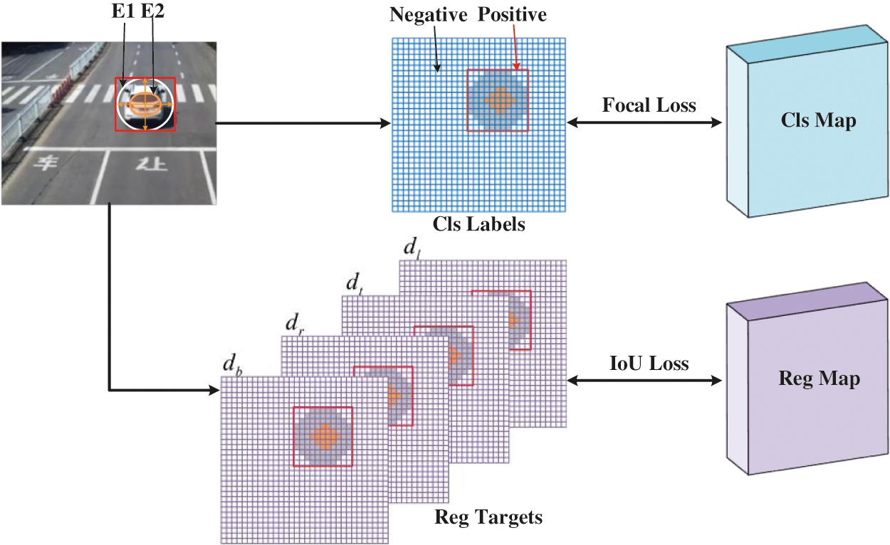
Figure 1: Illustration of classification labels and regression targets. The predicted value and monitoring signal are shown in the figure, where E1 represents ellipse E1 and E2 represents ellipse E2. Focal loss and IoU loss were used for classification and regression respectively

Taking the center point of the bounding box (xc(i),yci) w/4, h/4 as the center and the axis length, respectively, obtain the ellipse E2:\

x=(x−xc(i))2(w4)2+(y−yc(i))2(h4)2=1 (2)

If the position (x, y) falls within the ellipse, it is marked as a positive sample Bei , if it falls outside the ellipse E1, it is marked as a negative sample Bgi , if it falls in the middle of the ellipse E1 and E2, ignore it. The position (x, y) regresses the bounding box, and the regression target is expressed as:

dl=x−x0(i)dt=y−y0(i) (3)

dl=x1(i)−x  db=y1(i)−y (4)

Here dl,dt,dr,db betoken the distance from the position (x, y) to the left, top, right, and bottom of the bounding box. In training, the loss function utilized in this paper is shown as the following:

L({px,y},{tx,y})=1Npos∑x,y⁡Lcls(px,y,cx,y∗)+γNpos∑x,y⁡l{cx,y∗>0}Lreg(tx,y,tx,y∗) (5)

Where Lcls denotes focal loss, Lreg betokens IOU loss, Npos denotes the number of positive samples Bei , γ is set as the balance weight of Lreg to 1 and l{cx,y∗>0} represents for the indicator function, in the case of cx,y∗>0 , the value of which is 1, otherwise equals to 0. px,y and tx,y are points (x , y) classification function and regression function, while cx,y∗ , tx,y∗ betoken the class label and the position of the point (x, y).

3.2 Center Branch

A fully convolutional network is composed of a backbone network and two subnets divided by tasks. As shown in Fig. 2, the backbone network is a ready-made convolutional network, which mainly computes the convolutional feature graph of images. The first subnetwork is mainly based on the characteristics of the judgment as to which class it belongs to, The second subnetwork is to judge the specific position of the boundary box. Between the backbone network and the two subnets, the FPN is constructed by the backbone network, which has a hierarchy from to, I being the pyramid level and 1/2I resolution of the input image. FPN uses a top-down architecture with horizontal connections to build a pyramid of features in the network from a single-scale input. Each layer of the pyramid can be used to detect objects of different scales.

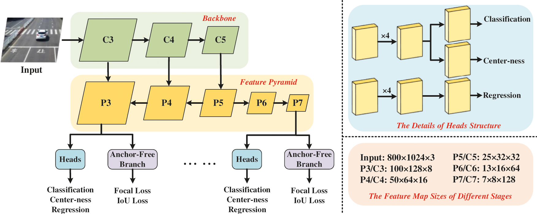
Figure 2: The fully convolutional network structure

In the structure proposed in this paper, a 3 × 3 convolutional layer with K filters is added to the feature map in the classification subnet, and then the sigmoid function, so that the object of K object classes at each spatial position can be predicted with probability. In addition, a 3 × 3 convolutional layer with four filters is added to the feature map of the regression subnet, and then the ReLU function is used to predict the box offset. After using FRN’s multi-level prediction, there will be multiple low-grade prediction bounding boxes far away from the center of the object. We propose an uncomplicated and profitable strategy to eliminate these low-grade detection bounding boxes without introducing any hyperparameters. Representatively, we have added a separate branch parallel to the classification branch (as shown in Fig. 2) to predict the centrality of a location.

The centrality is calculated by Eq. (6). When the position is far from the center of the object, the centrality attenuates from 1 to 0. In the test, multiplying the centrality predicted by the network by the classification score can reduce the weight of the low-grade bounding box predicted by the position far from the center of the object. The centrality describes the normalized distance from the location to the center of the object responsible for that location. The regression target for a given location is dl,dt,dr,db , and the centrality is defined as:

centerness=min(dl,dr)max(dl,dr)×min(dt,db)max(dt,db) (6)

The square root utilized here is to slow down the attenuation of centrality. The center is from 0 to 1, so training binary cross-entropy (BCE) loss. In the test, the final score is calculated by multiplying the predicted centrality by the corresponding classification score (used to sort the detected bounding boxes). Therefore, the center attribute can reduce the weight of the bounding box far from the center of the object, and finally use the NMS process to filter out these low-grade bounding boxes, which significantly strengthens the detection performance.

3.3 Dynamic Selection of Optional Feature

The ground truth output of the classification is K feature maps, and each feature map corresponds to a class. This example affects the k ground truth map in two ways. First, the effective frame Bei area is a positive area filled with an ellipse E2 , which indicates the existence of an instance. Second, ignore the area between ellipse E2 and ellipse E1, which signifies that the gradient of this area does not propagate back to the network. It should be noted that if two objects overlap at the same level, the smaller object is preferred. The remaining part is filled with black, indicating that it is a negative sample and there is no object. In the case of high parameters α = 0.25 and γ = 2.0, focal loss is used for monitoring. For an image, the total classification loss of an anchorless branch is the sum of the focal loss of all non-ignored areas, normalized by the total number of pixels in all valid frame areas.

The ground truth of the regression output is 4 offset mappings irrespective of the category. The instance only affects the Bei area on the offset map. Set the 4-dimensional vector of the (x, y) position on the 4 offset maps to Bi/S, and each map corresponds to a dimension. S is the normalization constant, we choose S = 4.0 based on experience. The position outside the effective frame is the area where the gradient is ignored. Optimized based on IOU loss. For an image, the total regression loss of an anchorless branch is the average of the IOU loss of all effective regions.

The anchorless design allows the use of the characteristics of any layer Pi of the pyramid to learn each instance. To find the best feature layer, we propose an innovative module of Dynamic Selection of Optimal Feature, which is referred to as the DSOF module for short. DSOF module can select the best Pi according to the content of the instance, rather than the size of the instance box like the anchor-based method.

Given an instance I, define its classification loss function and regression loss function on Pi as LFlI(i) and  LIOUI(i) respectively, which are calculated by calculating the average of the focal loss and IOU loss of the positive sample area Counted, namely:

LFlI(i)=1N(Bei)∑x,y∈Bei⁡FL(i,x,y) (7)

LIOUI(i)=1N(Bei)∑x,y∈Bei⁡IOU(i,x,y) (8)

where, N(Bei) is the number of pixels in the region of  Bei , and LFlI(i,x,y) and LIOUI(i,x,y) and are the focal loss and IOU loss of position (x, y) on Pi, respectively.

Fig. 3 shows the process of dynamic selection of features. First, pass the instance I through all levels of the feature pyramid, then use formula 9 to calculate the sum of LFlI (i) and LIOUI(i) , and finally select the pyramid Pi learning instance with the smallest loss, that is:

L∗=argminLFl′(i)+LIOUl (9)

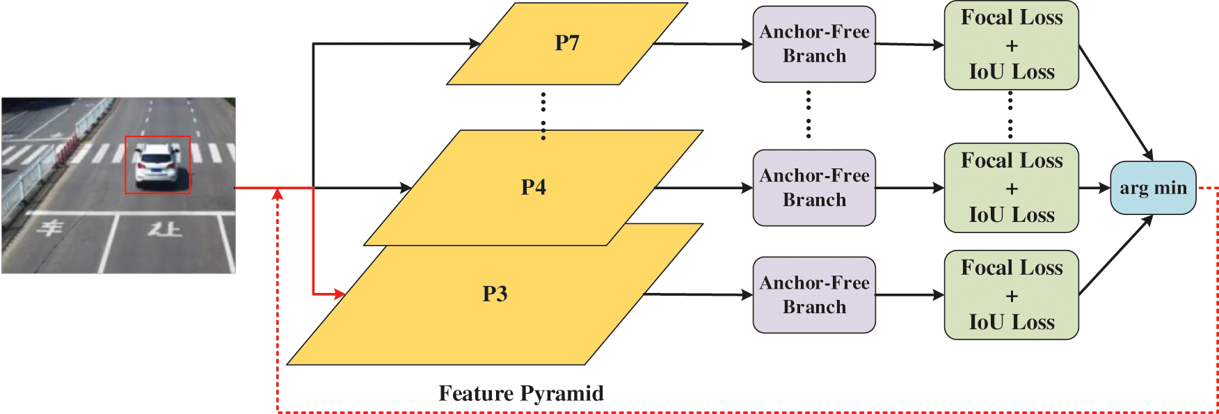
Figure 3: The dynamic selection module of the optimal feature

For training batches, the features will be updated for their corresponding assigned instances. Intuition tells us that the selected feature is currently the optimal choice for modeling the instance. Its loss forms a lower limit in the feature space. Through training, this lower limit is further pulled down. During inference, there is no need to select features, because the most appropriate feature pyramid level will transparently output high confidence values.

4  Experiments

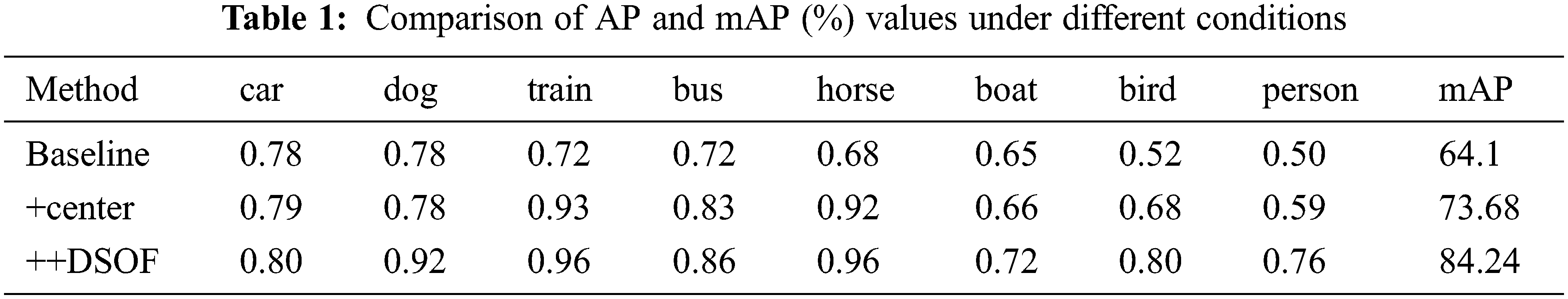
Pascal VOC [34] is the most commonly used data set for benchmarking target detection models. We conducted experiments on PASCAL VOC with 20 object categories. We train VOC2007 and VOC 2012 training models, speculate on the VOC2007 test set, and verify the VOC2007 validation set. The target detection accuracy is measured by the average accuracy of AP and mAP.

4.1 Experiments and Details

We use centrality and DSOF to evaluate our method, and the evaluation indicators are AP and mAP values, as shown in Tab. 1. The branch of centrality is necessary. We have trained the detectors with or without center branches. It turns out that the center branches have greater performance, mAP is strengthened by about 9%, and the overall AP value is higher. Selecting the correct feature learning plays a fundamental role in detection. We trained the model with or without the DSOF module. The experimental sequences indicate that the mAP value of the detector with the DSOF module has enlarged by about 11%. As can be seen from Fig. 4, DSOF is greater at finding small objects and objects that are susceptible to interference.

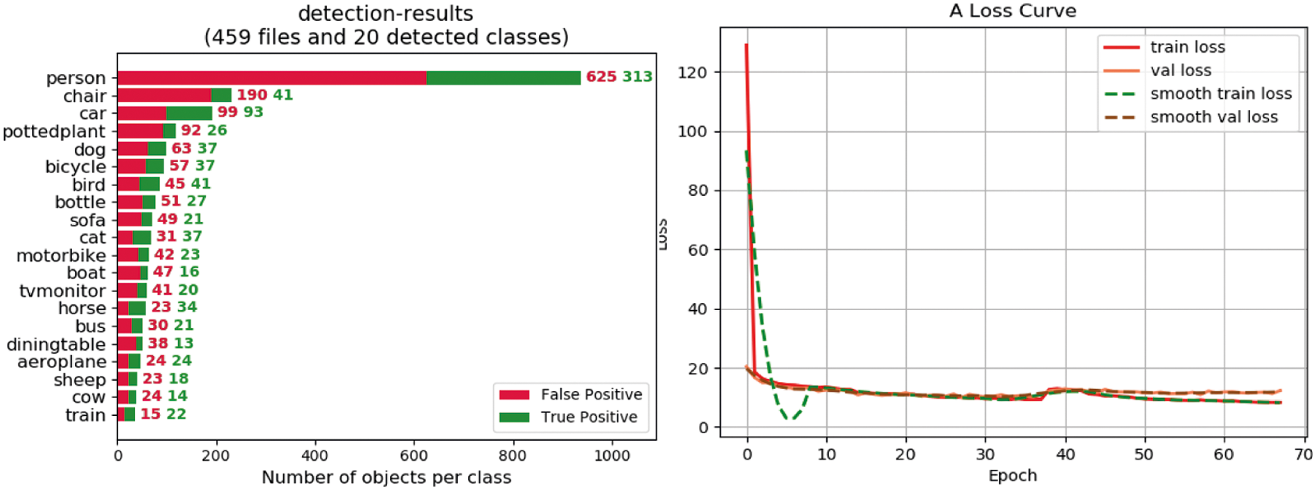
Figure 4: The figure on the left is the number of FP and TP for each target category. The figure on the right is the convergence of various loss functions

To better understand the pyramid level of optimal feature selection, we visualize some detection sequences from Fig. 5. The picture on the bottom uses our method. It is easier to detect objects that are not easy to detect, such as a table, and a zebra similar to the background. Fig. 4 shows the number of false positives and true positives in the detection training. The figure on the right indicates the convergence of train loss, val loss, smooth train loss, and smooth val loss as the number of epochs enlarges. When the number of iterations reaches more than 10, The loss function starts to converge, and the values tend to be close to 8.

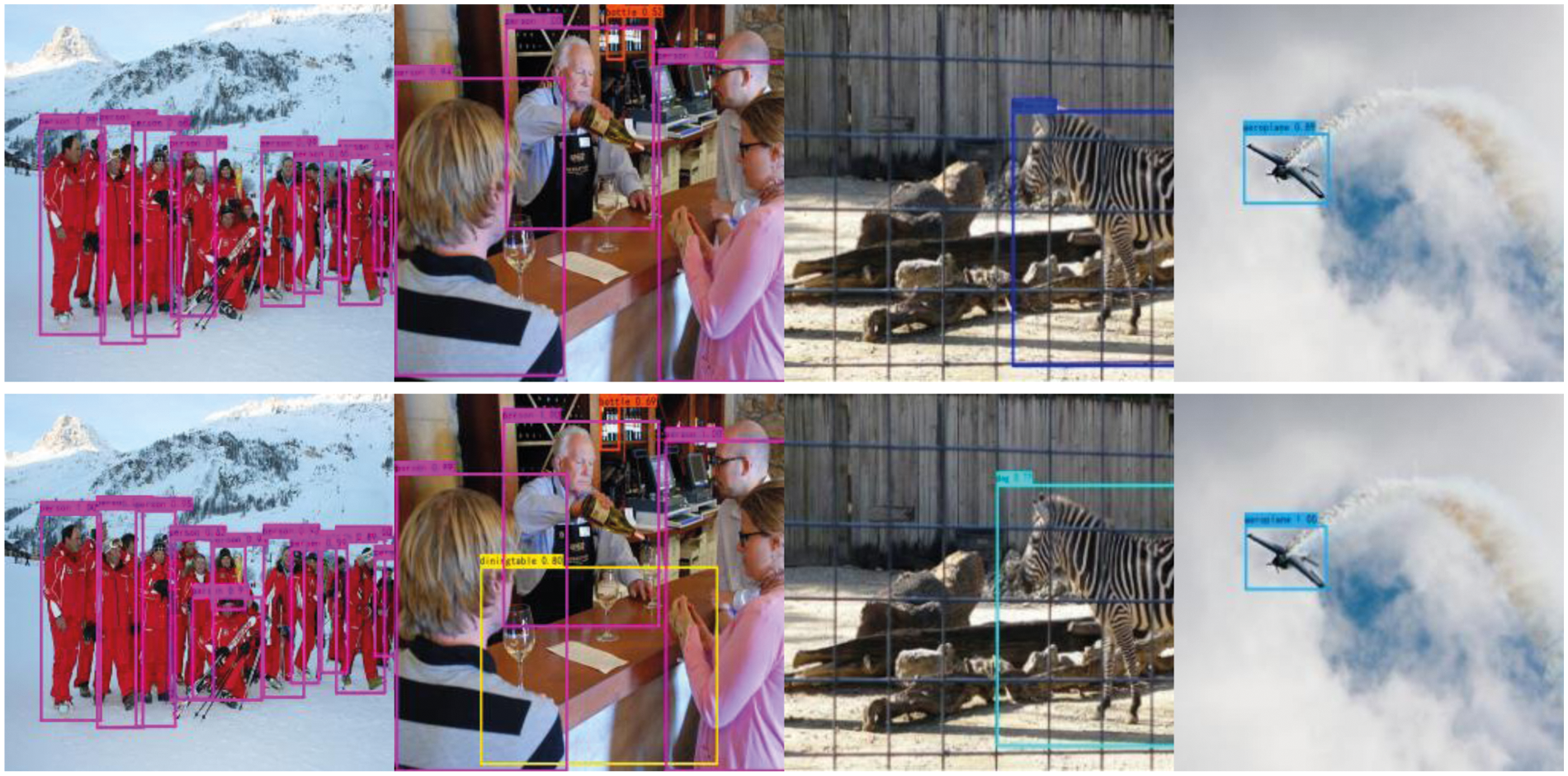
Figure 5: Both are using ResNet-50 as the backbone. The bottom is our method's sequents, and the top is the detection sequences of the yolov3 algorithm. Our DSOF module helps find more pick-and-shovel objects, such as small objects and easily disturbed objects

See Tab. 2 below, on the horizontal axis of the curve, Recall represents the proportion of the sample with a predicted value of 1 and a true value of 1 in all the samples with a true value of 1, namely, the true positive rate, which reflects the coverage ability of the classifier on positive samples. The recall is the ratio of correct Ground Truth to all Ground Truth, that is, Recall = TP/(TP+FN), TP is truly positive, FN is a false negative, and the denominator of Precision on the vertical axis is the number of positive cases identified. Not the actual number of positive examples. Precision represents the proportion of the sample with the predicted value of 1 and the true value of 1 in all the samples with the predicted value of 1, which reflects the accuracy of the classifier to predict positive cases. Precision is targeted at a certain type of sample.

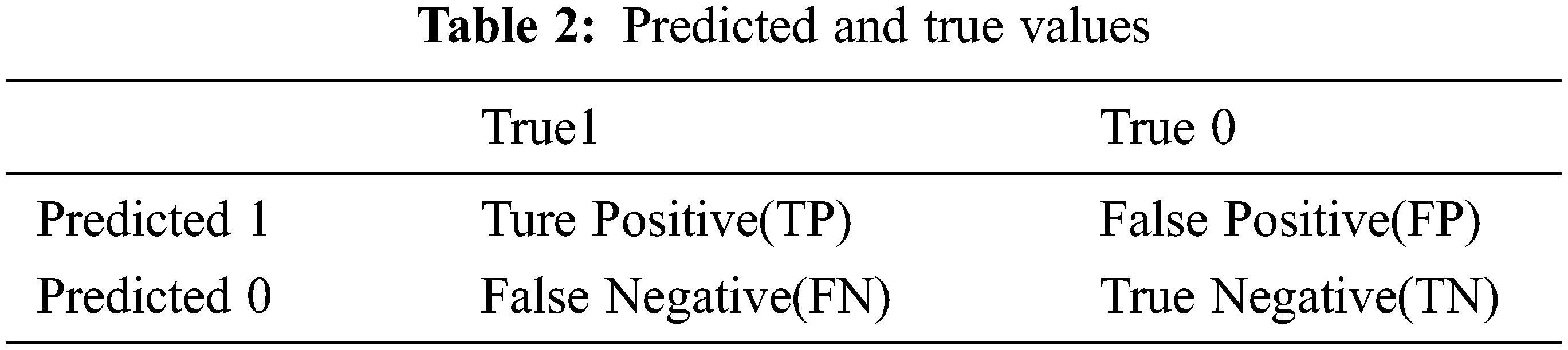
Precision = TP/(TP+FP), FP is false positive. Then, the precision-recall curve reflects the tradeoff between the recognition accuracy of positive cases and the coverage ability of positive cases. For a random classifier, its Precision is fixed equal to the proportion of positive examples in the sample and does not change with the change of recall. A PR curve can be drawn for each category of multiple categories. In the curve, a set of coordinates composed of precision and recall can be obtained by changing the confidence of 10%-100% in sequence, and these values are connected as PR curves. Fig. 6 below shows PR curves of eight different categories. The top two lines are the detection results without a centered algorithm, while the bottom two lines represent the detection results with the centered algorithm. It can be seen intuitively that the AP values with center branches are higher.

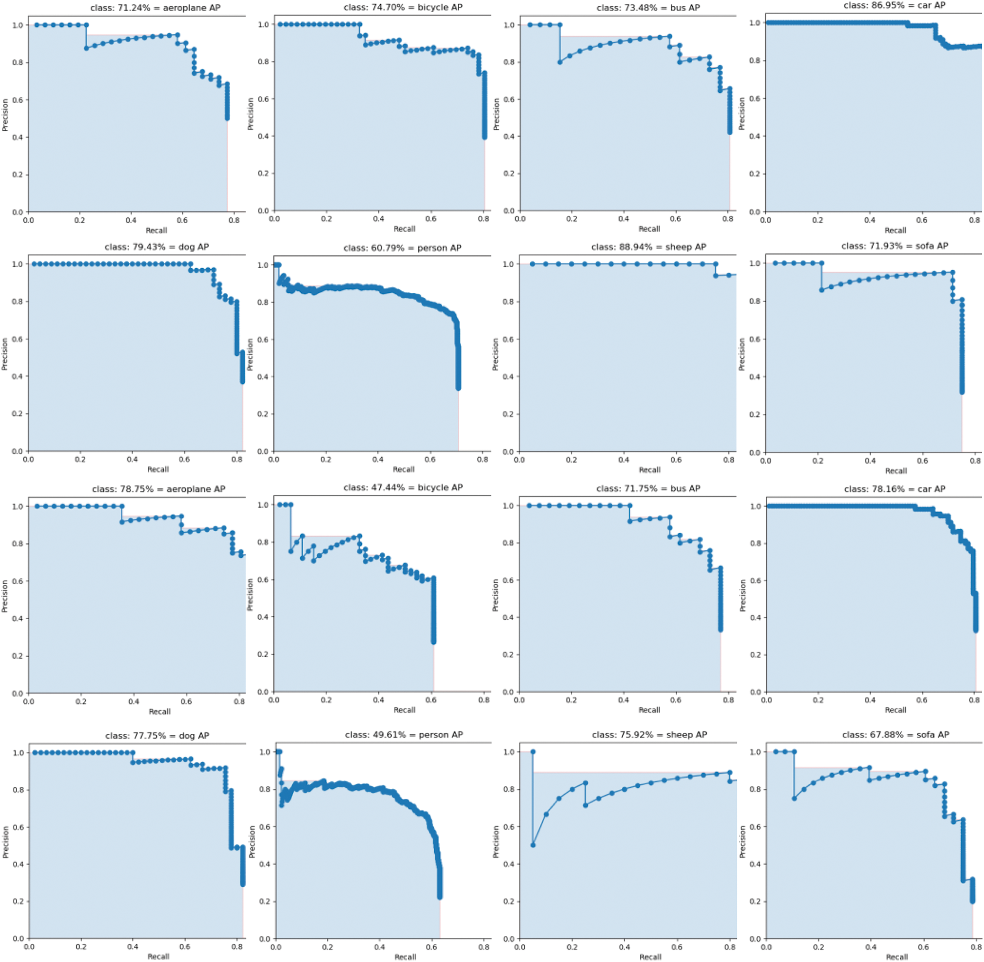
Figure 6: PR curves for each category

F1 Score is defined as the average of Precision and Recall, also known as balanced score. The specific formula is: F1=2∗(Precision∗Recall)/(Precision+Recall) . It is an index used to measure the accuracy of dichotomous or multi-task dichotomous models in statistics, and it takes into account both the accuracy and recall rate of classification models. F1 score can be regarded as a weighted average of model accuracy and recall rate, with a maximum value of 1 and a minimum value of 0. A larger value means a better model. As shown in Fig. 7, the upper two rows represent the F1 score of the model without centrality, and the lower two rows represent the F1 score of the model with centrality added.

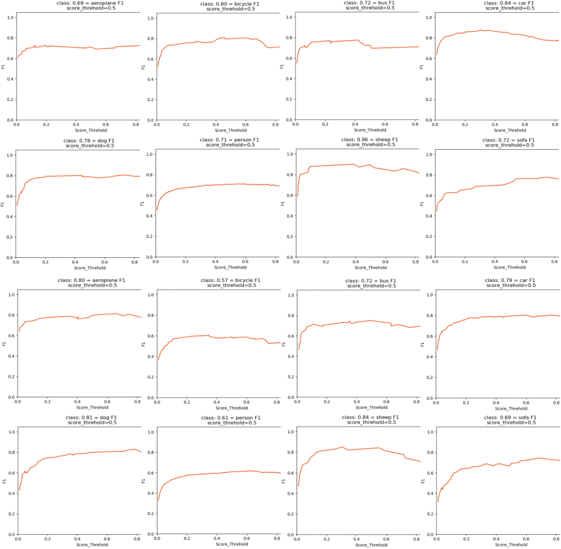
Figure 7: F1 scores for each category

We can learn from Fig. 6 that the bottom two lines represent the detection results without the centerness algorithm, while the top two lines represent the detection results with the centerness algorithm. It can be seen intuitively that the AP values with center branches are higher.

4.2 Comparison to State of the Art

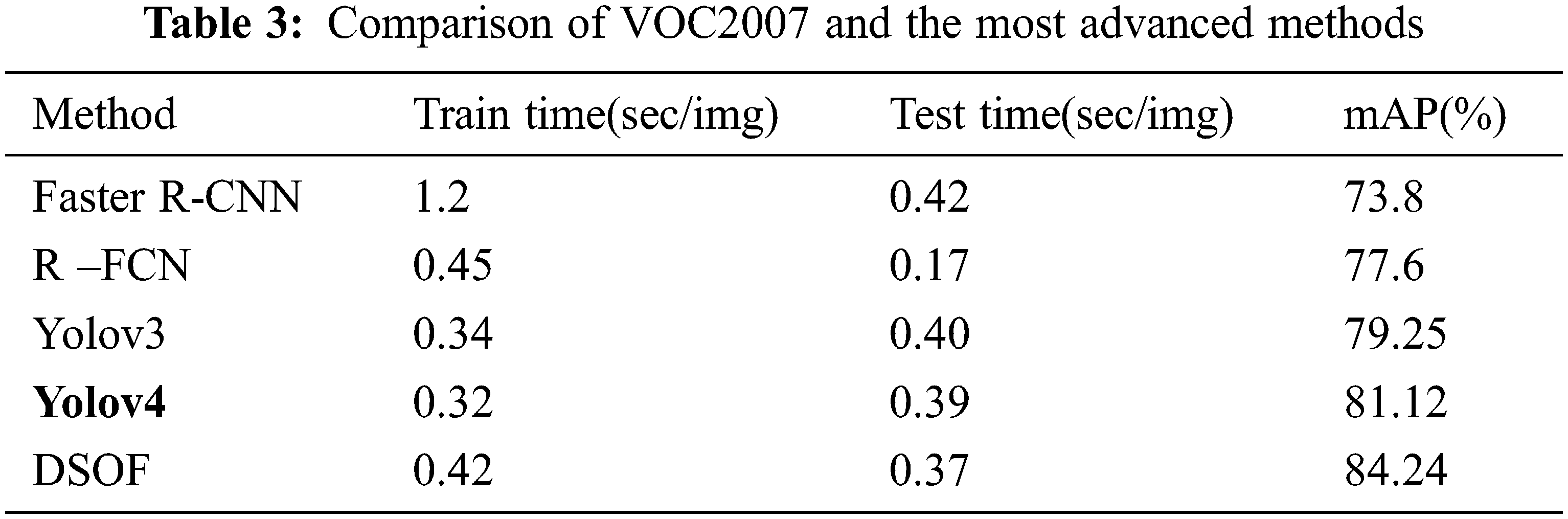
In Tab. 3 we compare DSOF and the most advanced methods in target detection. The final model is a fully convolutional network with a DSOF module, the training time and testing time of each image, and the mAP value of various methods. As can be noticed that the mAP value of our method is significantly higher than that of Faster R-CNN and other algorithms, the training time and test time of each picture are commensurately moderate, and there is no enlargement.

5  Conclusion

In target detection, we have proposed a simple and effective DSOF method. This module applies real-time online feature selection to train anchorless branches in the feature pyramid, avoiding all calculations and hyperparameters related to anchor boxes, and predicting pixel by pixel. The method solves the target detection, adds the center branch, and strengthens the judgment method of positive and negative samples. The experiment proves the persuasiveness of our method.

Acknowledgement: The author would like to thank the researchers in the field of object detection and other related fields. This paper cites the research literature of several scholars. It would be difficult for me to complete this paper without being inspired by their research results. Thank you for all the help we have received in writing this article.

Funding Statement: This work was supported National Natural Science Foundation of China (Grant No. 41875184) and the innovation team of “Six Talent Peaks” in Jiangsu Province (Grant No. TD-XYDXX-004).

Conflicts of Interest: The authors declare that they have no conflicts of interest to report regarding the present study.

This work is licensed under a Creative Commons Attribution 4.0 International License, which permits unrestricted use, distribution, and reproduction in any medium, provided the original work is properly cited.