DOI:10.32604/iasc.2022.025609
| Intelligent Automation & Soft Computing DOI:10.32604/iasc.2022.025609 | |
| Article |
CAD of BCD from Thermal Mammogram Images Using Machine Learning
1Department of Computer Science and Engineering, Paavai Engineering College, Pachal, Namakkal, 637018, Tamil Nadu, India
2Al-Nahrain University, Al-Nahrain Nanorenewable Energy Research Center, Baghdad, Iraq
3COMBA R&D Laboratory, Faculty of Engineering, Universidad Santiago de Cali, Cali, 76001, Colombia
4Department of Electronics and Communication Engineering, KPR Institute of Engineering and Technology, Coimbatore, 641048, Tamil Nadu, India
5Department of Mathematics, Jaypee University of Engineering and Technology, Guna, 473226, Madhya Pradesh, India
*Corresponding Author: D. Banumathy. Email: baanumathyd@gmail.com
Received: 30 November 2021; Accepted: 14 January 2022
Abstract: Lump in the breast, discharge of blood from the nipple, and deformation of the nipple/breast and its texture are the symptoms of breast cancer. Though breast cancer is very common in women, men can also get breast cancer. In the early stages, BCD makes use of Thermal Mammograms Breast Images (TMBI). The cost of treatment can be severely reduced in the early stages of detection. Based on the techniques of segmentation, the Breast Cancer Detection (BCD) works. Moreover, by providing a balanced, reliable and appropriate second opinion, a tremendous role has been played by ML in medical practices due to enhanced Information and Communication Technology (ICT). For the purpose of making the whole detection process of Malignant Tumor (MT)/Benign Tumor (BT) very resourceful and time-efficient, there is now a possibility to form an automated and precise Computer-Aided Diagnosis System (CADs). Several Image Pattern Recognition Techniques were used to classify breast cancer using Thermal Mammograms Image Processing Techniques (TMIPT) in the present investigation. Presenting a new model to classify the BCD with the help of TMIPT, thermal imaging, and smart devices is the aim of this research article. Using well-designed experiments like Intensive Preoperative Radio Therapy (IPRT) and BCD, the implementation and valuation of a concrete application are carried out. This proposed method is for the automatic classification of TMBI of a similar standard so that the thermal camera of FLIR One Gen 3 One 3rd Generation (FLIR One Gen 3) that can be attached to the smart devices are capable of capturing BCD using Machine Learning (ML) algorithms. To imitate the behaviour of human Artificial Intelligence (AI), designing drug formulations, helping in clinical diagnosis and robotic surgery systems, finding medical statistical datasets, and decoding human diseases’ wireless network model as well as cancer are the reasons for the ML to empower the computer and robots. The outperformance of the ML models against all other classifiers and scoring impressively across heterogeneous performance metrics like 98.44% of Precision, 98.83% of Accuracy, and 100% of Recall are observed from the comparative analysis.
Keywords: Breast cancer detection; machine learning; image processing techniques; artificial intelligence; thermal mammograms
The ducts’ lining cells (epithelium) (85%)/lobules (15%) in the breast's glandular tissue is the place from where Breast Cancer (BC) originates. Primarily, in the duct/lobule (“in situ”) where there are no symptoms and less possibility of spread (metastasis), the growth of cancer is limited [1–5]. In 2021, the most frequently diagnosed cancer type in the world is BC. In 2021, across the world, more than 2.26 million new BC cases and around 6,85,000 deaths caused du to BC were estimated by International Agency for Research on Cancer (IARC) during October 2021. The common reason for the death of women was breast cancer, and overall, it was the 5th most common reason for cancer death. Cranio-Caudal and Medio-Lateral Oblique are the two major kinds of BC. The ducts or tubes that take milk to the nipple, and the lobules that produce milk are where the BC usually appears. Though BC is unusual in males, it occurs both in men and women. Curing cancer by giving effective treatment is highly possible in the early detection of this disease. The slightest possibility of survival, high expensive treatments and even casualty are the results of the late detection of this disease [6].
When it comes to BCD, there are several IPRT. Magnetic Resonance Imaging (MRI) and X-radiation (X-ray) mammography with ultrasound scans are the most frequently used techniques for detecting cancer. Mammography with an ultrasound scan and magnetic resonance imaging that play a supportive role are is the gold standards of these recommended methods. A technique that is non-invasive, forthright, non-contact skin surface temperature screening, fast, cheap and not imposing any pain on the patient, is known as thermography.
The normal and abnormal functioning of the vascular system of the body, sensory and sympathetic nervous system and inflammatory processes are exposed by thermogram [7]. There are more chances for treatment and fewer chances of fatality (25.0%) when BCD is detected and diagnosed in the initial stages. But the precise segmentation of the breast Region Of Interest (ROI) [8], which is a significant part of CAS [9], is the basis of tumour detection. The disease is detected/diagnosed using multiple tools. Computer-Aided Diagnosis (CADx) and Computer-Aided Detection (CADe) systems can be used to reduce this cost. The medical diagnosis can be made using various techniques and approaches viz., CADe. Database, data analysis, Machine Learning (ML), and Image Processing (IMPRO). A false negative between 10% to 90% and sensitivity between 70% to 90% are testified by mammography. Many segmentation techniques that are at present used in mammogram segmentation like ML, DL and classical segmentation exist [10].
In saving human lives, the initial stages of Breast Cancer Detection (BCD) help much. Besides, the most renowned and straightforward method of the initial stage BCD has been the classification of mammography. An accuracy of more than 90% in mammography is predicted by radiologists. A comprehensive understanding of the learning process and implanting learning skills in the CADe system are achieved using ML, which is a sub-field of AI [11–15].
The enhancement of new CAD-IPRT to classify cancer/non-cancer TMBI from mammogram images is included in the primary aim of this research work.
a) For the classification of BC and noncancerous images, many IMPRO techniques are developed from these mammogram images. Thermal imaging detects the aspects of BC using smart devices.
b) For quick detection of BCD, the ML algorithms are used to build the predictive model for improving the prognosis and possibility of survival by giving the patients with appropriate clinical treatment.
c) The ML algorithm is used as an input to extract segmentation and classification features of TMBI.
The organization of this research article is as follows. Section 1 introduces various factors and reasons for cancer, and Section 2 contains different traditional methodologies available to detect cancer cells from thermal mammogram images. Section 3 shows a complete background of this research, such as detection of breast cancer, and BCD measurement by self-evaluation test with breast cancer diagnoses like mammogram, breast ultrasound and MRI scan. Section 4 consists of proposed thermography image processing techniques for BCD, and image classification has been done through CAD-TMIPT. This also contains various machine learning models for classifying mammogram images. Section 5 discusses the different results for the dimensionally-modelled relational database with the proposed algorithm to detect abnormalities in images. The conclusion and future work are discussed in Section 6 for thermal mammogram images.
Neural Network (NN) for BCD has been implemented by [16–20]. To automatically decompose a problem CAD and solve it, a negative correlation training algorithm was used. Two approaches, viz., ensemble and evolutionary approach, have been discussed by the author. The compact NN is designed automatically using an evolutionary system. Though the enormous problems were tackled by the ensemble model, it was still in progress.
The genetic algorithm and Backpropagation NN that were established as a quick classifier model are combined for reducing the diagnosis time and also for maximizing the precision while categorizing mass in breast to BT/MT using a computerized BDC developed by [21]. On the dataset, these two distinct processes were carried out. The records with missing values are alone eliminated in Set ‘A’, whereas with the usual statistical cleaning process, Set ‘B’ was trained so that the noisy/missing values can be identified. Finally, a maximum accuracy percentage of 100% was given by Set ‘A’, and an accuracy of 83.36% was given by Set ‘B’. Since the highest percentage of accuracy is given by medical data when compared to modified data, the author has thus decided that the best place to keep medical image data is in its original value.
By comparing Artificial Neural Networks (ANNs) with Logistic Regression (LR), an article has been submitted by [22]. The key covariates that cause an impact on death due to cancer, Disease Recurrence with the help of Area Under Receiver-Operating Characteristics (AUROC) and Disease-Free Survival (DFS), are identified by the author by comparing multi-layer perceptron NNs with Standard Logistic Regression (SLR). An article on BC's survival analysis on two BC datasets has been presented by [23]. As communication of variables can be easily considered and a non-linear prediction model can be created by ANNs, when compared to conventional methods, the ANNs can give a very flexible prediction of survival time. The two distinct BC datasets that use nuclear morphometric features are used in this investigation to compare the ANN results. The successful prediction of recurrence possibility and classification of patients with a good and bad prediction by ANN are explicit in the results.
The Mammogram Image Pre-processing (MIP) was enhanced using the method proposed by [24]. There are II-phases in the method: Phase I: the pixel brightness was used for removing the extra image parts; and Phase II: the positioning of Mammogram Images (MI) should be unidirectional. Besides, the threshold limit is used to remove the noise from the MI. The algorithm is tested using a sum of 60 test images obtained from the MIAS database. A segmentation accuracy of 99.0% was produced by the proposed method.
To track microcalcifications on MI, a comparison was made on the segmentation algorithms. The 250 MI that was obtained from the MIAS database was used to examine the method. This study made use of mean segmentation, mean shift, and watershed. The watershed segmentation has the ability to have an accurate detection of 18.0% and false detection of 94.0%. Contrarily, means segmentation can give a correct detection of up to 42.8% and false detection of up to 57.2%. On the basis of Hidden Markov and region growing, predicted pectoral muscle removal and BC segmentation. The separation of feature extraction from BC and pectoral muscles from MI is the scope of the proposed method. There are two stages in this method: (a) The thresholding concept of Otsu and (b) the means based on image classification. The MIAS database provides the MI. An accuracy of 91.92% and an error of 8.07% were reported, respectively.
The masses in mammography are detected using the threshold segmentation method proposed by [25]. In this method, the morphological threshold helps to detect a region of mass. The mini-MIAS database that provided 55 mammograms was utilized to examine this method, and a contrast limited adaptive histogram equalization and median filter enhanced the mammograms. 94.54% was the segmentation accuracy, and 5.45% was the False Positive Rate (FPR). The region merging and global thresholding were used by [26] in their proposed BC segmentation method. The Wiener filtering was used to remove the Gaussian noise, and based on the histogram shrinkage, image normalization was carried out. The masses from the ROI were segmented by applying global thresholding using the method of Otsu. For obtaining the ROI, a MATLAB simulation setup on 50 MI enabled the implementation and investigation of the proposed method. An accuracy of 82.0% and an error rate of 18.0% were produced by the proposed method.
3.1 Detection of Breast Cancer
The methodology of this research is focused in this section-to identify the factors that predict BCD; a geographical comparison of BC is provided using the gathering of tools and techniques on the basis of applying big data mining approaches. BC that accounts for 14% of all cancers, is the most common cancer in Indian women. The data of Globocan 2018 reported the following: (a) New cancer cases: 1,62,468, and (b) Fatality: 87,090 [27–30].
In the early thirties, the incidence rates in India started to increase, reaching the peak of the ages between 50–65 years. During the lifetime, 1 in 28 women is more likely to develop BC. When compared to rural areas, where 1 in 60 women develops BC in their lifetime, which is lesser than urban areas where 1 in 22 women is more likely to develop BC in a human lifetime. Tumours can be either malignant (cancerous) or Benign (noncancerous). The breast cells are the starting point of the BC, which is the BT/MT. There may be slow growth of BT, but it never spread, whereas the normal tissues nearby can be grown quickly, invaded and destroyed by the MT. Both men and women are affected by this, but men rarely get this. Specialized milk-producing glands are contained in a woman's breast. 15–20 lobes are comprised in the breast structure. So many smaller lobules that have a group of tiny milk-producing glands form each lobe. The reservoir that is located below the nipple is where the network of tiny tubes (duct) take the milk to. The areola is the dark round area of skin around the nipple. Blood and Lymph Vessels (LV) and Lymph Nodes (LN) are also contained in the breast. The lymphatic system is one of the main ways through which BC spreads [31–35].
Lymph is a clear fluid that drains into LN and is carried by LV. LV is a small bean-shaped structure that comprises infections fighting cells in the LN. The axillary lymph nodes and supraclavicular LN are the places where the LV from the breast drains. Overall, most women are affected by BC, which is the commonest cancer among Indian women. The following information is for the female BCs. In India, due to BC, 1,62,468 new cases are have been registered, and 87,090 deaths have been reported [36–40].
3.2 Breast Cancer Detection Measurement
An X-ray of the breast is taken using a mammogram. It is a common method for screening BC. In the mammogram, if there is any detection of abnormality, then a diagnostic mammogram may be recommended by the doctor in order to evaluate the abnormality further (Fig. 1). At its broader view, the primary BC's size is measured by the doctors. Usually, the size is given in millimeters (mm)/centimeters (cm).
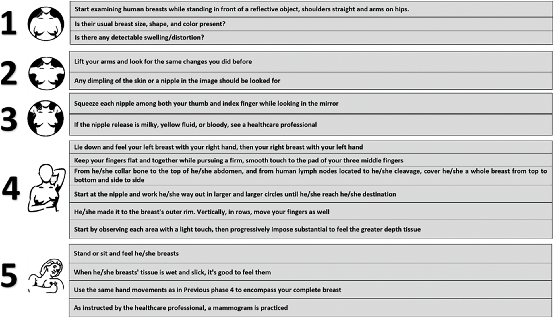
Figure 1: Self-evaluation test for humans to check BCD
(i) Early Detection (ED): Breast awareness, clinical breast detection and diagnosis of mammography are included in ED methods for BC. The self-examination of breasts, a technique that was taught to women in the past, did not have any improved outcomes, and so it was not recommended anymore. Many men and women with BC have no symptoms, but sometimes it is found after symptoms appear. For this reason, the regular detection and diagnosis of BC are very crucial [41].
(ii) Clinical Breast Examination (CBE): After 30 years, every human is recommended to CBE once a year. Health professionals like doctors, nurses/medical social experts examine human breasts using CBE, which is a medical investigation of the breasts. At first, the breasts will be carefully examined by the healthcare professionals for any abnormal changes in the nipple, like the skin, size/shape. Next, to check the presence of any lumps, the healthcare professionals will palpate human breasts using their fingers. Also, any swelling in LN under both arms will also be examined by humans [42].
(iii) Breast Self-Examination (BSE): A clear idea of how human breasts look like should be known. If any abnormality is noticed in the breast, get a timely medical recommendation. To find out the early signs of BC in men and women who are above 20 years, BSE is recommended [43].
(i) CBE: The under-arm region of the breasts ispalpated by a doctor to find any lumps. In case any skin changes, retraction and discharge are suspected, then the nipples are examined [44].
(ii) Imaging Tests
• Mammogram: A low-dose X-rays are used by a mammography machine for taking images of the breast. Initially, each breast is compressed and is taken X-ray images on film by the machine.
• Breast Ultrasound: High-frequency sound waves are sent through the breast in this process. The tissues that send the sound signals are transformed into images on the computer screen. The doctor is then allowed to discover the abnormality in-these images.
• MRI Scan: In this process, particularized images of the breast and the neighbouring organs are scanned and created using a high-powered magnet and a computer. Only in particular cases where the information provided by a mammogram is inadequate, breast MRIs are recommended.
i) Staging of Breast Cancer
• The lesion/lump/tumour's size
• Whether the breast has only been affected by cancer
• Whether to any other human organs, cancer has spread, except the breast
ii) Staging of Tumor Node Metastasis (TNM)
• Size of tumour (T-Tumor)
• Involvement of LN (N-Node)
• Whether cancer has metastasized (M-Metastasis)/spread to the rest of the body parts.
4 Proposed Thermography Image Processing Techniques for Breast Cancer Detection
The set of Thermography Image Mammogram Technique (TIMT) applied for generating an image for its utilization in the rest of the proposed work is known as IMPRO. By offering CAD of BC, TIMT is crucial in its attempt to assist practitioners in the field. The CAD systems that mainly concentrate on BC are used by several IMPRO techniques on the basis of the concrete approach and purpose. The adoption of CADe in medical diagnosis is defined as CAD. Multiple models and techniques like IMPRO, database, big data analysis, and ML are combined in this detection and diagnosis. The BCD is used as input MRI/other images by most of the CADe that facilitates it. In order to be an input to a CADe, first of all, the images should be in an apt digital format. For the excellence of the final result, the TIMT step is pivotal in spite of whether they are acquired from mammography. As a result, often digitizing the present mammogram or MRI, which is stored in analogue format, is the prime task of TIMT. But since the performance of the successive TIMT improves the image quality, it later identifies, differentiates or else marks on the image elements or attributes of interest [45–55].
The depreciation in assets and plant location is located with the help of thermography, which is a non-destructive evaluation method for detecting and measuring minute differences in temperature. With its quick and cost-saving application of thermography, it can protect industrial plants and equipment.
Maintaining the categorization of the cancerous and noncancerous images from TMBI to use IMPRO and ML strategies is the prime objective of this research study. In Fig. 2, the TMIPT categorizes the attribute and recognize the cancerous and noncancerous image provided by the flow chart. Here, the 120 quantities of TMBI assist the creation of the proposed CAD-TMIPT. Out of these, 60 images belong to cancerous/noncancerous images. The framework is executed using the computer software programming that is developed in MATLAB simulation programming. There are three main phases of tumours recognition in mammograms. The image optimization strategies to optimize an image are included in the primary phase. To make specific attributes less challenging and further expand them, the Signal to Noise Ratio (SNR) is performed by these strategies by changing colours or brightness. Then, the confirmation of brightness is an ultimatum of image values to the next reach. In Section 3, the test that archived the image collected from TMIPT has been discussed. The segmentation of the image background and feature extraction from every segmented image were carried out in the IMPRO segment [56–61].
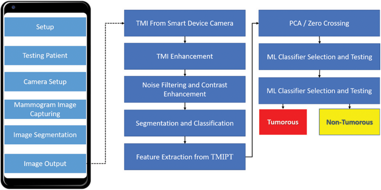
Figure 2: CAD-TMIPT and classified TMBI's proposed work
Heterogeneous factors are taken into account for an InfraRed (IR) image quality, and non-controlling of these factors results in thermal artifacting in the image that badly affects the trustworthiness of the image. It asserts that “the usual procedures minimize the quantity and impact of variables, facilitate interpretation and sharing of knowledge, and impose trustworthiness.” Mainly, the past poor results were due to the absence of standard procedures. The medical TMBI is captured and stored prior to the reappraisal studies that would primarily stick to their own control protocols. There was no sufficient control over the images of the research studies, and also it would give negative results. So, this was not ideal [62–67].
From then onwards, stringent standardizations have been made not only for breast thermography but for all dimensions of thermography. An outline of the standards to be adhered prior to the examination of a patient, the process and situation in which the examination was done, and the acquired thermograms’ post-processing are given. Many factors are included in the standards like (a) getting the patient ready, (b) environment of examination, (c) thermal imager systems’ standardization, (d) protocol of image capturing, (e) protocol of image analysis, and (f) reporting, archiving, and storing.
The least necessities for the attachable Forward Looking Infrared Radiometer (FLIR) One Gen 3rd are described by the client-side model. The standards of FLIR One Gen 3rd should be more than the least necessities and the best one of the time. The capturing of exact images will lead to an appropriate thermographic examination when there is proper control of the patient and environment, and the FLIR One Gen 3rd camera is fixed correctly. The image is investigated from this instant onwards so that there can be a classification of classes where a diagnosis can be made.
4.3 Thermal Mammogram Image Contrast Techniques
The same usual manner of processing thermographic data is the Thermal Mammogram Image Contrast-Techniques (TMICT). Several TMICT definitions are in existence, and the necessity for a good area Sa is shared by most of them, i.e., a non-defective area that comes under the view of the field. For example, the definition of the total TMBI ΔTt is as in following Eq. (1):
Pixel p's temperature (defective/not) is TMBId(Time) / the group of pixels’ average value, and the temperature at the time ‘t’ for the Si is
After the pulse has been set up, the prime thing is defining ‘t’ as a given time value between the instant and when the first defective spot is found in the thermogram sequence, the moment is precise, i.e., detection of defect when there is sufficient contrast. Yet, the presence of a defect is not indicated at ‘t’. Hence, like the defective area, there is the same local temperature for a Si, Eq. (2).
The complete TMICT definition substituted by Eq. (3) is as follows:
Eq. (3) provides the original measurements diverge from the optimum solution for the future when the thickness of the plate increases with regards to the non-semi-infinite case. Nonetheless, since the DA-TMICT curtails the artefacts due to the non-uniform heating and surface geometry, it has been determined to be effective also for anisotropic materials at the early period.
A slight difference is shown by the TMICT profiles for distinct places at an early period (up to 1 s), and later on, they deviate. To extend the authenticity of the DA-TIC result to a later period, an altered DA-TMICT has been proposed. The DA-TMICT cogency was extended to future times by apparently including the plate thickness L in the solution by the finite plate model and the thermal quadrupoles theory. This is the base of the proposed DA-TMICT model. The solution of the form is obtained using the Laplace inverse transform:
where the Laplace variable is ‘Lp’.
4.4 Machine Learning Models and Classification
The ML and the methods suitable for breast thermography are discussed in this section. The different kinds of ML systems are discussed at the beginning, with more emphasis on supervised learning. The qualitative or categorical data are dealt with by the classification problems. Classification of observation is nothing but anticipating a qualitative response. To classify observations, one can use many techniques that are called classifiers. The factors like what is meant by classification, how it is done, the usual problems faced, and also a few renowned classifiers are detailed in this section. Since classification algorithms are directly associated with the problem that is addressed in the research, they are later discovered and introduced. There is an introduction to Computer Vision (CV) and a description of its association with breast thermography giving an emphasis on converting raw TMBI into feature sets with the capability of giving it to an ML algorithm for classification. Also, the calculation of different features from TMBI is also discussed.
A. Gradient Boosting Machine (GBM): The least-squares at each iteration fit the simple parameterized function systematically to the existing “pseudo”-residuals so that GBM builds additive regression models. Otherwise, during the training process, the model's loss function always descends in the gradient direction. In various differentiable loss functions, GBM can be applied. The frequently raised problems like classification, regression and also ranking can be handled using various loss functions. GBM is indeed effective though it appears to be the most brute-force learning method. In supervised learning, BCD is a classical regression problem. The implementation of the encapsulated GBM is easy so that it can work as a “baseline” model.
B. Distributed Random Forest (DRF): Until Breiman first proposed this algorithm, the DRF classification had been a sort of popular ensemble learning since 2001. A description of how the classification and Regression Trees (RT) are constructed is changed by DRF rather than contracting each tree with a distinct bootstrap dataset. Only two parameters are required by the DRF algorithm: the need for the number Ndt of Decision Trees (DT) to be constructed and the number Nif of input features to be taken into account in case each node of the decision tree is divided.
i) Let the number of training examples be Ndt. Then for a single decision tree, the number of input samples for a DT is Ndt. The Ndttraining samples are recovered from the training set.
ii) Let Nifbe the training examples’ number of input features, and Nifis larger than cut m. Next, at each node of DT, the m input features from each of the Nifdivide the m input features randomly, and the best one is divided to select one of the ‘m’ input features. During the decision tree construction, ‘m’ does not change.
iii) Until this time, each decision tree has been divided till all the training sample datasets for that node are of the same category. There is no need for pruning.
C. eXtreme Gradient Boosting (XGB): The tree boosting method that has been believed to be an extremely efficient ML method is to which XGB belongs. The sparser data are processed using XGB, which is an enhanced and scalable system, and it can be appropriated into an extensive range of situations. RT is the basic unit of the Boosting Tree (BT). Based on the input attributes of image features, it allocates input to each child node, and an actual score is contained in each child node. Very remarkably, the possibilities of the expected result are indicated by the score below the child.
D. Deep Learning Neural Network (DLNN): The other word for Deep Learning (DL) is ANN that is the foundation of AI. The biological NNs’ structure inspires the structure and single components. In the NN, every single unit is presented as a perceptron whose logic features are as same as the biological neuron. The weight is similar to a synapse, and the function's bias can be similar to the threshold voltage. Then there is a surprising similarity in the output of the observations and the biological neuron. Once the complex connections between perceptions are recognized, the part of the functions of the cerebral cortex is stimulated so that the NN can function as an energetic system.
Nonlinear, non-limited, qualitative and non-convex are the features of the system. The data must be fed into the neural net's input layer once the hierarchy structure and the connections are determined and the outcome is acquired from the output layer. The framework and the hyperparameters like rate of learning, the output activation function and the hidden layer number absolutely determine the efficiency and the precision. In a gene sequence, the genetic features can be seen as attributes with regard to the BCD problem. Image, audio records and Natural Language Processing (NLP) are the aspects worked excellently by the NN in addition to feature detection. Also, genetic feature detection may work well.
E. Logistic Regression (LR): Also, the logistic/logit model is known as LR. When the target variable is a categorical variable, for instance, active/inactive, healthy or unhealthy, then this type can be used. The data are fitted into an LR curve to predict the possibility of an event occurrence with the help of LR.
750 samples and 32 features that belong to the atomic features measured visually from a digitized image of a breast mass’ Fine Needle Aspirate (FNA) are contained in the dataset. The FNA that collects a sample for diagnosing/anticipating disease like cancer is a thin needle inserted into the body fluid or tissues that look abnormal. 338 MT and 412 BT are the classifications of the 750-sample dataset. The TMBI of the breast mass is from where the features are mined. The specification on how the precision of the methods deployed for classification differs on the basis of a few parameters is provided by the plots given below. The size of the training dataset is 500, and the test dataset is 350. The ML repository supplies the BC dataset.
The Dimensionally-Modeled Relational (DMR) database from where the example of normal and abnormal thermograms are extracted is shown in Fig. 3. In patients having one breast, the abnormal patient TIBI is removed from examination because the patient is not absolutely straight or the TIBI is badly out of focus that leads to the image artefacts by the capture device. The selection by TIBI of 30 patients was made for the analysis of asymmetry to match the 30 abnormal patients.
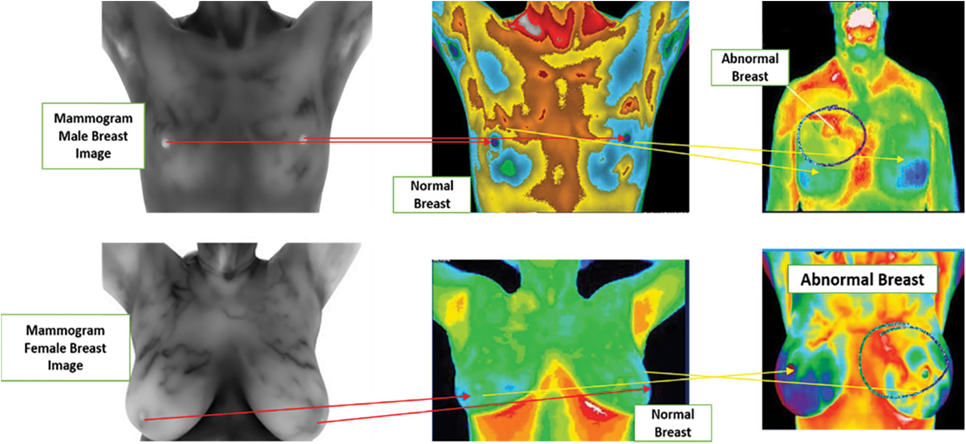
Figure 3: Thermograms breast image with normal vs. abnormal for human
From each one of the cells in the sample, the following ten features are computed:
• TIBI environment
• TIBI surface
• TIBI edge
• Smoothness of TIBI
• Compression of TIBI
• TIBI curved inward
• TIBI's curved inward boundaries
• Balance of TIBI
• TIBI's Fractal Measurements
30 features are the result of the computation of mean, standard error and “worst”/bulkiest of these features. For example, Radius SE is field 13, Worst Radius is field 23, and Mean Radius is field 3. The four crucial digits are used to record all feature values. No missing values are found in this dataset. Both numerical and categorical features are present in the dataset. The categorical features are consisted only in the ‘Tumor Diagnosis’ column that is going to anticipate if it is MT/BT. The remaining is numerical features.
On using bars of various heights, where numbers are grouped by each bar into ranges, a histogram graphically represents data or information. The grouping of more data in that range is shown by higher bars. A histogram can be used to shape and spread sample data persistently. 338 MT is present that is 38% on average, and the rest of the 412 BT makes 64.56% of the predictive class. In Fig. 4, we can see that the nucleus features can be plotted against diagnosis from which the cell radius’ mean values, area, perimeter, concave points, concavity, and compactness can be utilized in breast cancer classification.
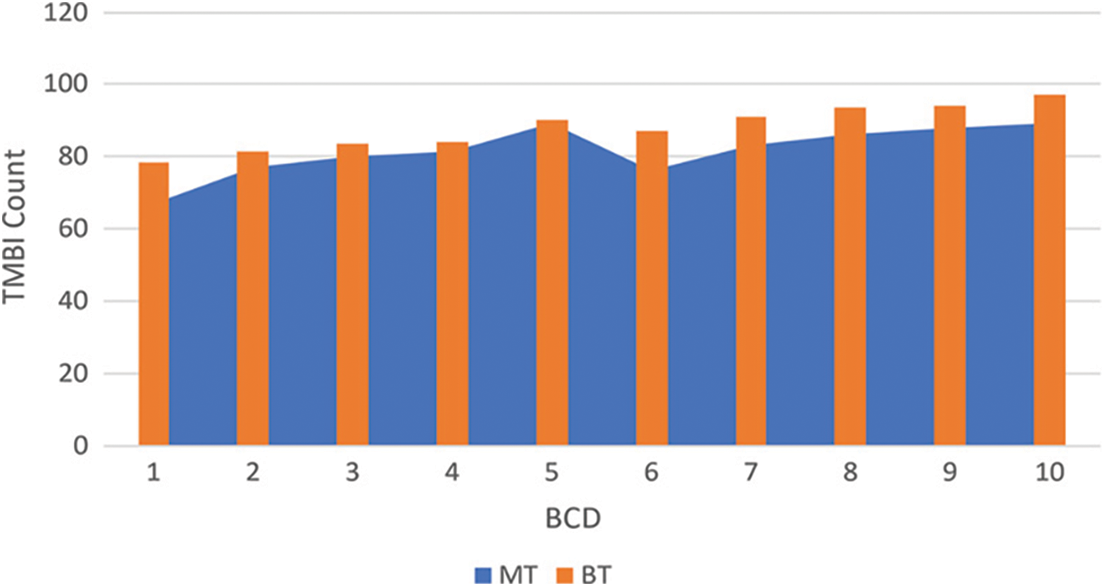
Figure 4: Class distribution of BT/MT
The correlation with MT is shown by greater values of these parameters. A specific choice of one diagnosis over the other is not shown by the mean values of smoothness, texture, fractal dimension/symmetry. The large differentiable outliers, which need a further clean-up, do not exist in any of the histograms.
A. Heatmap: Both detailed and straightforward information are visualized using colours in a heatmap, which is a 2D representation. For finding out the intersections that have values with higher data concentration, the heatmap is comparatively highly useful. The heatmap enabled correlation matrix is represented by Fig. 5. In the dataset, the correlation among all 30 features is shown using a heatmap.
B. Confusion Matrix (CM): The model's prediction vs. the target classes is organized using a model called CM. In a predicted class, each row of the matrix that represents the instance is described. The finding of whether this model is perplexing the classes is done efficiently using this method. For binary classification, Tab. 1 shows a CM in order to be easy.
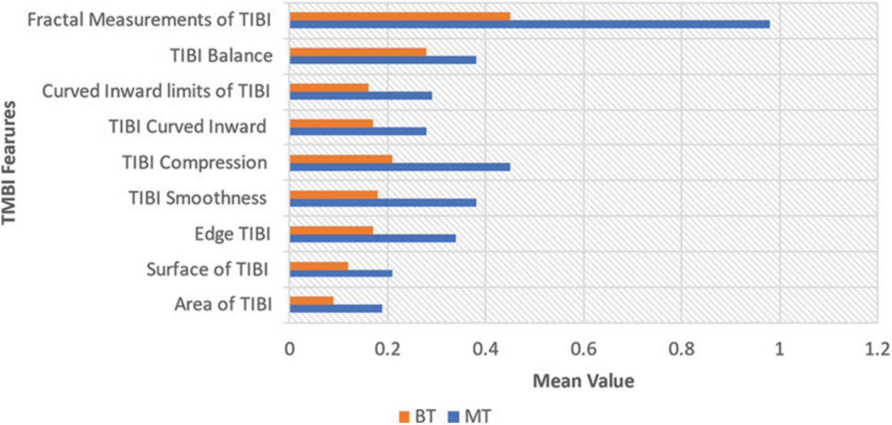
Figure 5: Features of growth and metabolism vs. BCD

True Positive (TP), True Negative (TN), False Positive (FP), and False Negative (FN) are the terms of CM (Fig. 6). The correct classifications are TP and TN; When the prediction was true, but the target was False, FP occurs; When the prediction was False, and the target was True, FN occurs.

Figure 6: Correlation between all variables
To extract useful data, a zero-cross distribution is used in our zero-crossing algorithm. In our learning process, we possess the input data after producing a new matrix with a zero-crossing count. An output vector that has been created manually with 0's for normal images and 1's for BC data is required by this algorithm. But a normalization process should be employed on the input data prior to the utilization of these input data.
5.1 BCD Steps Involved in Zero Crossing Algorithm
Step 1. Initialize
Step 2. iMage(i) RGB of TMBI;
Step 3. iMage is the CM of Gray Values;
Step 4. N is Total Number TMBI;
Step 5. Begin
Step 6. CH, CV CD = Coefficient of CM of Image Wavelet Transformation
Step 7. FS Total Features Set of TMBI
Step 8. FS[i] Size of CM i
Step 9. For All, i = 1 to N
{
IMage = Gray(iMage(i));
CH,CXV,CD = iMage wavelet(iMage);
}
Step 10. For a = FS[iMage]/FS
{
Step 11. For b = FS
{
Step 12. If (a > 0 && a − 1 < 0) OR a < 0 && a − 1 > 0) Then
{
Count = Count + 1;
Step 13. }
Step 14. End If
Step 15. }
Step 16. }
Step 17. End For
Step 18. End For
Step 19. End For
Step 20. End Process
In this section, the proposed ML model is described, and the execution that includes the dataset visualization, preprocessing of data, the proposed algorithms’ brief background, train-test split and Principal Component Analysis (PCA) are explained in its subsections (Fig. 7). The dimension-reduction minimizes a massive set of variables to a small set yet consists of predominant information in the large set, which is performed by the PCA. Basically, PCA is a mathematical process where many correlated variables are converted into a few uncorrelated linear variables known as principal components using an orthogonal transformation. PCA was deployed for LR, DLNN, XGB, DRF, and GBM classifiers after data standardization. The dataset is minimized to 10 principal components from the preceding 40 features that represent each observation once the PCA is applied.
A. GBM: In Fig. 7, after PCA is applied on the dataset, it is discovered that much difference is not found between GBM's confusion matrix and the model's GM. 95.78% is the Accuracy. There is an improvement of Precision and F1 scores at 95.68% and 94.59%, respectively. More than Precision, the Recall is significant in BCD, also at its highest of 96.18%. 99.35% is the AUC that is mainly compared with other conventional metrics for this model.
B. DRF: 95.68% is the accuracy of the DRF model once the 10-folds cross-validation is applied, and the accuracy has reduced acutely to 91.32% while applying PCA and standardization. 95.28% is the precision of the objective performance metrics along with Accuracy, 96.79% is Precision, and 97.84% is the F1 score once PCA is introduced and that can indicate the model's CM prior to PCA.
C. XGB: With the small size of the dataset, XGB performs comparatively well for an NN resulting in 98.67% Accuracy with 95.17% of high Precision and a 97.19% F1 score. In BCD, since the cost involved in missing a positive is problematic, the cost of adding a negative Recall is very crucial than Precision. A perfect Recall score of 99.34% is given by this model. The 99.19% of the ROC curve and the Area Under the Curve (AUC) are shown in Fig. 7.
D. DLNN: Nearly all the ML algorithm has been outperformed by ANN; however, there are certain limitations, such as the requirement of a huge dataset and high computing power. As seen in Fig. 7, which demonstrates the CM for the DLNN model, the performance of DLNN is outstanding in spite of the small-sized image dataset. This model produces 98.83% Accuracy, 99.14% high Precision and 98.45% F1 score. In this model, the Recall is very significant than Precision in BCD, achieving a 99.67% Recall score. 99.19% is the ROC curve and the AUC.
E. LR: The LR model's CM with and without PCA employed on the dataset is illustrated in Fig. 7. Primarily, after 10-fold cross-validation, 97.35% is the model's Accuracy with 98.38% as AUC score. Unlike the other models, after deploying PCA to the dataset, there is a substantial rise in the Accuracy of up to 98.19% with 99.28% of AUC score that exemplifies the LR model's ROC curvewith PCA. With 98.12% Precision, 96.15% Recall and 97.34% F1-Score, the results demonstrate the performance of LR for this problem.
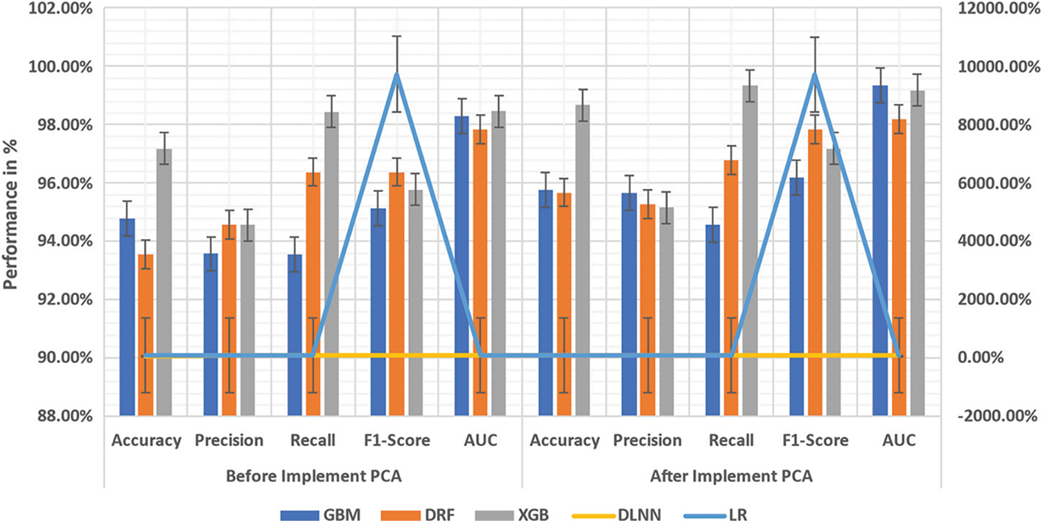
Figure 7: ML's performance comparison (GBM, DRF, XGB, DLNN, LR)
From Tabs. 2 and 3, the GBM and DRF's performance that falls throughout all the metrics in the post-order of PCA can be understood. At the same time, there is a decline in the Accuracy, Precision and Recall scores of XGB, which are 95.32%, 95.74%, 95.32% etc. DRF replaces DLNN because the latter performs worse with PCA with 89.32% of Accuracy, 90.38% of Precision, and 89.32% of Recall. But LR has achieved 97.68% at the lowest compared to ANN with a lack of PCA though its performance with PCA is outstanding; however, there is still 97.68% lower precision when compared to ANN with lack of PCA.


An overview of the BT/MT of the problem is agreed by 70% of death associated with breast cancer that is the most common cancer among men and women and the same gender. By getting timely clinical treatments, the ED of BC results in the chances of survival of a huge number of these people. There are three contributions to the existing knowledge: First, the CADe systems that facilitate BCD is to which an outline of current IPRT is used; Finding features in the data, which are capable of distinguishing normal samples from those consisting of tumours, is the prime objective of the paper. Second, TMIPT, TMBI, and ML algorithms are used by the proposed method for automated BCD. From the FNA of a breast mass, this distinct ML algorithm in BCD is extracted from a digitized image. The complicated and effective ML algorithms and huge data matrices are controlled using TMICT, which is frequently used to process thermographic data, and the delicate and rapid combination of FLIR One Gen 3 IR cameras with dynamic computers are feasible. Promising results for a neighbouring seamless BCD system are shown by the performance of the ML models.
After comparing with the other approaches, this thesis can be prolonged, and at last, a BCD system with outstanding performance is built with the best one. The feature can be extracted optimally for more extraordinary performance when this article does not consider the extraction process.
Funding Statement: This research has been funded by the Research General Direction at Universidad Santiago de Cali under call No 01-2021.
Conflicts of Interest: The authors declare that they have no conflicts of interest to report regarding the present study.
Reference
1. N. Kavya, N. Usha, N. Sriraam, D. Sharath and P. Ravi, “Breast cancer detection using non-invasive imaging and cyber-physical system,” in 3rd IEEE Int. Conf. on Circuits, Control, Communication and Computing (I4C), Bangalore, India, pp. 1–4, 2018. [Google Scholar]
2. J. Dabass, S. Arora, R. Vig and M. Hanmandlu, “Segmentation techniques for breast cancer imaging modalities-a review,” in 9th IEEE Int. Conf. on Cloud Computing, Data Science & Engineering (Confluence), Noida, India, pp. 658–663, 2019. [Google Scholar]
3. P. Singh, S. P. Singh and D. S. Singh, “An introduction and review on machine learning applications in medicine and healthcare,” in IEEE Conf. on Information and Communication Technology, Allahabad, India, pp. 1–6, 2019. [Google Scholar]
4. S. S. Prakash and K. Visakha, “Breast cancer malignancy prediction using deep learning neural networks,” in 2nd Int. Conf. on Inventive Research in Computing Applications (ICIRCA), Coimbatore, India, pp. 88–92, 2020. [Google Scholar]
5. P. J. G. Lisboa, H. Wong, P. Harris and R. Swindell, “A Bayesian neural network approach for modelling censored data with an application to prognosis after surgery for breast cancer,” Artificial Intelligence in Medicine, vol. 28, no. 1, pp. 1–25, 2003. [Google Scholar]
6. S. U. Amin, M. Alsulaiman, G. Muhammad, M. A. Mekhtiche and M. Shamim Hossain, “Deep learning for EEG motor imagery classification based on multi-layer CNNs feature fusion,” Future Generation Computer Systems, vol. 101, pp. 542–554, 2019. [Google Scholar]
7. A. Makandar and B. Halalli, “Threshold-based segmentation technique for mass detection in mammography,” Journal of Computers, vol. 11, no. 6, pp. 472–478, 2016. [Google Scholar]
8. S. Dehghani and M. A. Dezfooli, “A method for improve preprocessing images mammography,” International Journal of Information and Education Technology, vol. 1, no. 1, pp. 90–93, 2011. [Google Scholar]
9. S. E. I. El Kaitouni, A. Abbad and H. Tairi, “A breast tumors segmentation and elimination of pectoral muscle based on hidden markov and region growing,” Multimedia Tools and Applications, vol. 77, no. 23, pp. 31347–31362, 2018. [Google Scholar]
10. X. Feng, L. Song, S. Wang, H. Song, H. Chen et al., “Accurate prediction of neoadjuvant chemotherapy pathological complete remission (PCR) for the four subtypes of breast cancer,” IEEE Access, vol. 7, pp. 134697–134706, 2019. [Google Scholar]
11. Y. Wang, N. Wang, M. Xu, J. Yu, C. Qin et al., “Deeply-supervised networks with threshold loss for cancer detection in automated breast ultrasound,” IEEE Transactions on Medical Imaging, vol. 39, no. 4, pp. 866–876, 2020. [Google Scholar]
12. G. Alexandrou, N. Moser, K. T. Mantikas, J. R. Manzano, S. Ali et al., “Detection of multiple breast cancer esr1 mutations on an ISFET based lab-on-chip platform,” IEEE Transactions on Biomedical Circuits and Systems, vol. 15, no. 3, pp. 380–389, 2021. [Google Scholar]
13. R. Roslidar, A. Rahman, R. Muharar, M. Rizky Syahputra, F. Arnia et al., “A review on recent progress in thermal imaging and deep learning approaches for breast cancer detection,” IEEE Access, vol. 8, pp. 116176–116194, 2020. [Google Scholar]
14. I. Iliopoulos, S. D. Meo, M. Pasian, M. Zhadobov, P. Pouliguen et al., “Enhancement of penetration of millimeter waves by field focusing applied to breast cancer detection,” IEEE Transactions on Biomedical Engineering, vol. 68, no. 3, pp. 959–966, 2021. [Google Scholar]
15. S. Jabbar, F. Ullah, S. Khalid, M. Khan and K. Han, “Semantic interoperability in heterogeneous IoT infrastructure for healthcare,” Wireless Communications and Mobile Computing, vol. 2017, no. 1, pp. 1–10, 2017. [Google Scholar]
16. R. Vasanthi, O. I. Khalaf, C. A. T. Romero, S. Sudhakar and D. K. Sharma, “Interactive middleware services for heterogeneous systems,” Computer Systems Science and Engineering, vol. 41, no. 3, pp. 1241–1253, 2022. [Google Scholar]
17. A. Mehbodniya, S. Bhatia, A. Mashat, E. Mohanraj and S. Sudhakar, “Proportional fairness based energy-efficient routing in wireless sensor network,” Computer Systems Science and Engineering, vol. 41, no. 3, pp. 1071–1082, 2022. [Google Scholar]
18. D. Stalin David, S. Arun Mozhi Selvi, S. Sivaprakash, P. Vishnu Raja, D. K. Sharma et al., “Enhanced detection of glaucoma on ensemble convolutional neural network for clinical informatics,” Computers, Materials & Continua, vol. 70, no. 2, pp. 2563–2579, 2022. [Google Scholar]
19. D. Stalin David, M. Anam, K. Chandraprabha, S. Arun Mozhi Selvi, D. K. Sharma et al., “Cloud security service for identifying unauthorized user behaviour,” Computers, Materials & Continua, vol. 70, no. 2, pp. 2581–2600, 2022. [Google Scholar]
20. K. Rajakumari, M. Vinoth Kumar, G. Verma, S. Balu, D. K. Sharma et al., “Fuzzy based ant colony optimization scheduling in cloud computing,” Computer Systems Science and Engineering, vol. 40, no. 2, pp. 581–592, 2022. [Google Scholar]
21. R. Nithya, K. Amudha, A. Syed Musthafa, D. K. Sharma, E. H. RamirezAsis et al., “An optimized fuzzy-based ant colony algorithm for 5G-MANET,” Computers, Materials & Continua, vol. 70, no. 1, pp. 1069–1087, 2022. [Google Scholar]
22. M. Rajalakshmi, V. Saravanan, V. Arunprasad, C. A. T. Romero, O. I. Khalaf et al., “Machine learning for modeling and control of industrial clarifier process,” Intelligent Automation & Soft Computing, vol. 32, no. 1, pp. 339–359, 2022. [Google Scholar]
23. J. F. C. García, J. H. Ortiz, O. I. Khalaf, A. D. V. Hernández and L. C. Rodríguez Timaná, “Noninvasive prototype for type 2 diabetes detection,” Journal of Healthcare Engineering, vol. 2021, no. 8077665, pp. 1–12, 2021. [Google Scholar]
24. O. I. Khalaf, G. M. Abdulsahib, H. D. Kasmaei and K. A. Ogudo, “A new algorithm on application of blockchain technology in live stream video transmissions and telecommunications,” International Journal of e-Collaboration (IJeC), vol. 16, no. 1, pp. 16–32, 2020. [Google Scholar]
25. A. D. Salman, O. I. Khalaf and G. M. Abdulsahib, “An adaptive intelligent alarm system for wireless sensor network,” Indonesian Journal of Electrical Engineering and Computer Science, vol. 15, no. 1, pp. 142–147, 2019. [Google Scholar]
26. K. A. Ogudo, D. M. Jean Nestor, O. I. Khalaf and H. D. Kasmaei, “A device performance and data analytics concept for smartphones’ IoT services and machine-type communication in cellular networks,” Symmetry, vol. 11, no. 4, pp. 593–609, 2019. [Google Scholar]
27. O. I. Khalaf and G. M. Abdulsahib, “Frequency estimation by the method of minimum mean squared error and P-value distributed in the wireless sensor network,” Journal of Information Science and Engineering, vol. 35, no. 5, pp. 1099–1112, 2019. [Google Scholar]
28. O. I. Khalaf and B. M. Sabbar, “An overview on wireless sensor networks and finding optimal location of nodes,” Periodicals of Engineering and Natural Sciences, vol. 7, no. 3, pp. 1096–1101, 2019. [Google Scholar]
29. G. M. Abdulsahib and O. I. Khalaf, “An improved algorithm to fire detection in forest by using wireless sensor networks,” International Journal of Civil Engineering and Technology (IJCIET), vol. 9, no. 11, pp. 369–377, 2018. [Google Scholar]
30. O. I. Khalaf and G. M. Abdulsahib, “Energy efficient routing and reliable data transmission protocol in WSN,” International Journal of Advances in Soft Computing and its Application, vol. 12, no. 3, pp. 45–53, 2020. [Google Scholar]
31. O. I. Khalaf, G. M. Abdulsahib and B. M. Sabbar, “Optimization of wireless sensor network coverage using the bee algorithm,” Journal of Information Science and Engineering, vol. 36, no. 2, pp. 377–386, 2020. [Google Scholar]
32. G. M. Abdulsahib and O. I. Khalaf, “Accurate and effective data collection with minimum energy path selection in wireless sensor networks using mobile sinks,” Journal of Information Technology Management, vol. 13, no. 2, pp. 139–153, 2021. [Google Scholar]
33. O. I. Khalaf and G. M. Abdulsahib, “Optimized dynamic storage of data (ODSD) in IoT based on blockchain for wireless sensor networks,” Peer-to-Peer Networking and Applications, vol. 14, no. 5, pp. 2858–2873, 2021. [Google Scholar]
34. R. Rout, P. Parida, Y. Alotaibi, S. Alghamdi and O. I. Khalaf, “Skin lesion extraction using multiscale morphological local variance reconstruction-based watershed transform and fast fuzzy C-means clustering,” Symmetry, vol. 13, no. 2085, pp. 1–19, 2021. [Google Scholar]
35. R. Surendran, O. I. Khalaf and C. Andres, “Deep learning-based intelligent industrial fault diagnosis model,” Computers Materials & Continua, vol. 70, no. 3, pp. 6323–6338, 2022. [Google Scholar]
36. O. I. Khalaf, M. Sokiyna, Y. Alotaibi, A. Alsufyani and S. Alghamdi, “Web attack detection using the input validation method: DPDA theory,” Computers, Materials & Continua, vol. 68, no. 3, pp. 3167–3184, 2021. [Google Scholar]
37. S. Palanisamy, B. Thangaraju, O. I. Khalaf, Y. Alotaibi, S. Alghamdi et al., “A novel approach of design and analysis of a hexagonal fractal antenna array (HFAA) for next-generation wireless communication,” Energies, vol. 14, no. 6204, pp. 1–18, 2021. [Google Scholar]
38. S. N. Alsubari1, S. N. Deshmukh, A. A. Alqarni, N. Alsharif, T. H. H. Aldhyani et al., “Data analytics for the identification of fake reviews using supervised learning,” Computers, Materials & Continua, vol. 70, no. 2, pp. 3189–3204, 2022. [Google Scholar]
39. S. Bharany, S. Sharma, S. Badotra, O. I. Khalaf, Y. Alotaibi et al., “Energy-efficient clustering scheme for flying ad-hoc networks using an optimized leach protocol,” Energies, vol. 14, no. 6016, pp. 1–20, 2021. [Google Scholar]
40. C. A. Tavera Romero, J. H. Ortiz, O. I. Khalaf and A. Ríos Prado, “Business intelligence: Business evolution after industry 4.0,” Sustainability, vol. 13, no. 10026, pp. 1–12, 2021. [Google Scholar]
41. N. Veeraiah, O. I. Khalaf, C. V. P. R. Prasad, Y. Alotaibi, A. Alsufyani et al., “Trust aware secure energy-efficient hybrid protocol for MANET,” IEEE Access, vol. 9, pp. 120996–121005, 2021. [Google Scholar]
42. N. A. Khan, O. I. Khalaf, C. A. T. Romero, M. Sulaiman and M. A. Bakar, “Application of euler neural networks with soft computing paradigm to solve non-linear problems arising in heat transfer,” Entropy, vol. 23, no. 1053, pp. 1–44, 2021. [Google Scholar]
43. N. Jha, D. Prashar, O. I. Khalaf, Y. Alotaibi, A. Alsufyani et al., “Blockchain-based crop insurance: A decentralized insurance system for modernization of Indian farmers,” Sustainability, vol. 13, no. 16, pp. 1–17, 2021. [Google Scholar]
44. O. I. Khalaf, C. A. T. Romero, A. A. J. Pazhani and G. Vinuja, “VLSI implementation of a high-performance non-linear image scaling algorithm,” Journal of Healthcare Engineering, vol. 2021, no. 6297856, pp. 1–10, 2021. [Google Scholar]
45. C. A. T. Romero, J. H. Ortiz, O. I. Khalaf and W. M. Ortega, “Software architecture for planning educational scenarios by applying an agile methodology,” International Journal of Emerging Technologies in Learning, vol. 16, no. 8, pp. 132–144, 2021. [Google Scholar]
46. O. I. Khalaf, “Preface: Smart solutions in mathematical engineering and sciences theory,” Mathematics in Engineering, Science and Aerospace, vol. 12, no. 1, pp. 1–4, 2021. [Google Scholar]
47. G. Suryanarayana, K. Chandran, O. I. Khalaf, Y. Alotaibi, A. Alsufyani et al., “Accurate magnetic resonance image super-resolution using deep networks and Gaussian filtering in the stationary wavelet domain,” IEEE Access, vol. 9, pp. 71406–71417, 2021. [Google Scholar]
48. G. Li, F. Liu, A. Sharma, O. I. Khalaf, Y. Alotaibi et al., “Research on the natural language recognition method based on cluster analysis using neural network,” Mathematical Problems in Engineering, vol. 2021, no. 9982305, pp. 1–13, 2021. [Google Scholar]
49. O. Wisesa, A. Andriansyah and O. I. Khalaf, “Prediction analysis for business to business (B2B) sales of telecommunication services using machine learning techniques,” Majlesi Journal of Electrical Engineering, vol. 14, no. 4, pp. 145–153, 2020. [Google Scholar]
50. A. T. Hoang, X. P. Nguyen, O. I. Khalaf, T. X. Tran, M. Q. Chau et al., “Thermodynamic simulation on the change in phase for carburizing process,” Computers, Materials & Continua, vol. 68, no. 1, pp. 1129–1145, 2021. [Google Scholar]
51. X. Wang, J. Liu, O. I. Khalaf and Z. Liu, “Remote sensing monitoring method based on BDS-based maritime joint positioning model,” Computer Modeling in Engineering & Sciences, vol. 127, no. 2, pp. 801–818, 2021. [Google Scholar]
52. C. A. Tavera Romero, D. F. Castro, J. H. Ortiz, O. I. Khalaf and M. A. Vargas, “Synergy between circular economy and industry 4.0: A literature review,” Sustainability, vol. 13, no. 8, pp. 4331 2021. [Google Scholar]
53. A. T. Hoang, X. P. Nguyen, O. I. Khalaf, T. X. Tran and M. Q. Chau, “Thermodynamic simulation on the change in phase for carburizing process,” Computers, Materials and Continua, vol. 68, no. 1, pp. 1129–1145, 2021. [Google Scholar]
54. G. M. Abdulsahib and O. I. Khalaf, “An improved cross-layer proactive congestion in wireless networks,” International Journal of Advances in Soft Computing and its Applications, vol. 13, no. 1, pp. 178–192, 2021. [Google Scholar]
55. G. M. Abdulsahib and O. I. Khalaf, “Accurate and effective data collection with minimum energy path selection in wireless sensor networks using mobile sink,” Journal of Information Technology Management, vol. 13, no. 2, pp. 139–153, 2021. [Google Scholar]
56. M. Krichen, S. Mechti, R. Alroobaea, E. Said, P. Singh et al., “A formal testing model for operating room control system using internet of things,” Computers, Materials & Continua, vol. 66, no. 3, pp. 2997–3011, 2021. [Google Scholar]
57. E. N. Al-Khanak, S. P. Lee, S. U. R. Khan, N. Behboodian and O. I. Khalaf, “A heuristics-based cost model for scientific workflow scheduling in cloud,” Computers, Materials and Continua, vol. 67, no. 3, pp. 3265–3282, 2021. [Google Scholar]
58. T. X. Tran, X. P. Nguyen, D. N. Nguyen, D. T. Vu, M. Q. Chau et al., “Effect of poly-alkylene-glycol quenchant on the distortion, hardness, and microstructure of 65 mn steel,” Computers, Materials and Continua, vol. 67, no. 3, pp. 3249–3264, 2021. [Google Scholar]
59. C. A. T. Romero, J. H. Ortiz, O. I. Khalaf and A. R. Prado, “Web application commercial design for financial entities based on business intelligence,” Computers, Materials and Continua, vol. 67, no. 3, pp. 3177–3188, 2021. [Google Scholar]
60. M. J. Awan, M. S. Mohd Rahim, H. Nobanee, A. Yasin, O. I. Khalaf et al., “A big data approach to black Friday sales,” Intelligent Automation and Soft Computing, vol. 27, no. 3, pp. 785–797, 2021. [Google Scholar]
61. O. I. Khalaf, K. A. Ogudo and M. A. Singh, “Fuzzy-based optimization technique for the energy and spectrum efficiencies trade-off in cognitive radio-enabled 5G network,” Symmetry, vol. 13, no. 1, pp. 1–47, 2021. [Google Scholar]
62. O. I. Khalaf, F. Ajesh, A. A. Hamad, G. N. Nguyen and D. N. Le, “Efficient dual-cooperative bait detection scheme for collaborative attackers on mobile ad-hoc networks,” IEEE Access, vol. 8, pp. 227962–227969, 2020. [Google Scholar]
63. S. Sudhakar, O. I. Khalaf, P. Vidya Sagar, D. K. Sharma, L. Arokia Jesu Prabhu et al., “Secured and privacy-based IDS for healthcare systems on e-medical data using machine learning approach,” International Journal of Reliable and Quality E-Healthcare (IJRQEH), vol. 11, no. 3, pp. 1–11, 2022. [Google Scholar]
64. S. Sudhakar, O. I. Khalaf, G. R. K. Rao, D. K. Sharma, K. Amarendra et al., “Security-aware routing on wireless communication for e-health records monitoring using machine learning,” International Journal of Reliable and Quality E-Healthcare (IJRQEH), vol. 11, no. 3, pp. 1–10, 2022. [Google Scholar]
65. S. Sudhakar, O. I. Khalaf, S. Priyadarsini, D. K. Sharma, K. Amarendra et al., “Smart healthcare security device on medical IoT using raspberry Pi,” International Journal of Reliable and Quality E-Healthcare (IJRQEH), vol. 11, no. 3, pp. 1–11, 2022. [Google Scholar]
66. S. Sudhakar, G. R. K. Rao, O. I. Khalaf and M. Rajesh Babu, “Markov mathematical analysis for comprehensive real-time data-driven in healthcare,” Mathematics in Engineering Science and Aerospace (MESA), vol. 12, no. 1, pp. 77–94, 2021. [Google Scholar]
67. S. Sudhakar, P. Vidya Sagar, R. Ramesh, O. I. Khalaf and R. Dhanapal, “The optimization of reconfigured real-time datasets for improving classification performance of machine learning algorithms,” Mathematics in Engineering Science and Aerospace (MESA), vol. 12, no. 1, pp. 43–54, 2021. [Google Scholar]
 | This work is licensed under a Creative Commons Attribution 4.0 International License, which permits unrestricted use, distribution, and reproduction in any medium, provided the original work is properly cited. |