DOI:10.32604/iasc.2022.025309
| Intelligent Automation & Soft Computing DOI:10.32604/iasc.2022.025309 | |
| Article |
Background Subtraction in Surveillance Systems Using Local Spectral Histograms and Linear Regression
1Coimbatore Institute of Technology, Department of Computer Science and Engineering, Coimbatore 641 014, India
2PSG College of Technology, Department of Computer Science and Engineering, Coimbatore 641 004, India
*Corresponding Author: S. Hariharan. Email: hariharan.s@cit.edu.in
Received: 19 November 2021; Accepted: 12 January 2022
Abstract: Background subtraction is a fundamental and crucial task for computer vision-based automatic video analysis due to various challenging situations that occur in real-world scenarios. This paper presents a novel background subtraction method by estimating the background model using linear regression and local spectral histogram which captures combined spectral and texture features. Different linear filters are applied on the image window centered at each pixel location and the features are captured via these filter responses. Each feature has been approximated by a linear combination of two representative features, each of which corresponds to either a background or a foreground pixel. These representative features have been identified using K-means clustering, which is used in background modeling using a least square method. Constraints have been introduced in the least square solution to make it robust in noisy environments. Experiments on existing datasets show that our proposed method outperforms the methods in the literature, with an overall accuracy of 92%.
Keywords: Intelligent surveillance system; spectral histogram; image processing; video processing; linear regression; background estimation; surveillance datasets
Background subtraction is often one of the first tasks in computer vision applications, and a crucial part of the system as well. Surveillance camera systems have been increasingly becoming more common, either for surveillance or information collection. Moreover, intelligent video monitoring is rapidly attracting researchers’ interest in building a smart city nowadays [1]. The increased number of camera systems has led to the development of software to process the images automatically. Detecting and tracking moving objects is the first step of any video analysis process, regardless of the area of use. Also, various practical tasks such as illegal parking warning, anomaly detection, smoke/fire detection, and so on, can often be accomplished by extracting the static video background and detecting the moving foreground object, which is then accompanied by individual detectors. The success of background subtraction is strongly influenced by the background modeling technique used.
The literature classifies the techniques for performing these operations into various categories. In general, these operations are either top-down or bottom-up [2]. In bottom-up methods, foreground objects are detected by defining special points or blocks of the current image and then classifying them using a previously trained model. Top-down methods, on the other hand, are those in which foreground objects are detected by determining the background of the image. Most of these methods perform well for videos consisting of a static background and stable environmental facts. However, for videos with complex scenes such as dynamic background, sudden light changes, shadow oscillations, and sleeping foreground objects, the problem remains difficult and under research. Natural scenes, in particular, place a high demand on background modeling since they are generally complex, with illumination transitions, swaying vegetation, rippling water, flashing monitors, etc. Also, a robust background modeling algorithm should be able to manage scenarios where new objects are added or existing ones are deleted from the background. Moreover, noise and camera jitter can cause frame-to-frame variations even in a static scene. In addition, the background modeling algorithm should be able to work in real-time.
A variety of methods for detecting moving objects have been proposed and to model the background, many different features are utilized. Most of these methods are pixel-based which uses only pixel color or intensity information and researchers have used several statistical models to describe background/foreground characteristics. In recent years, researchers have turned to exploring regional relationships among adjacent pixels using block-level processing and feeding their combinations into background extractors. Local Binary Patterns (LBP) and motion trajectories are common features extracted from the video and these features are the inputs to the background estimation technique to indicate the labels (background/foreground) of original pixels. These features are very limited in all types of images, especially, LBP has the drawback of not performing well on flat image areas like a sky where the gray values of adjacent pixels are very similar to the value of the center pixel. To the authors’ knowledge, none of the earlier studies have utilized discriminative combined spectral-texture features in dealing with the problem. In this paper, we propose an approach to handle the background estimation problem as a multivariate linear regression model and the solution has been obtained from least-square estimation. This uses powerful combined spectral-texture features referred to as the Local spectral histogram [3] to capture background statistics and motivation from the Incremental Iterative Re-weighted Least Squares (IIRLS) method presented in [4].
In general, a background subtraction algorithm constructs a reference background frame (background model) which represents the most static area of the frames throughout the scene and detects foreground objects by comparing an input image with the reference frame. Most of the conventional algorithms use pixel-level processing methods which approximate the intensity of each of the pixels individually using temporal statistics among consecutive frames to estimate the background of the scene. For example, the methods stated in [5,6] and [7] use average filtering, running average, and temporal-median filtering respectively. These methods are simple and fast, but very noise sensitive and require considerable memory storage to handle the frames used.
The most popular pixel-level processing method is to model each pixel of the image using a Gaussian distribution, which is the underlying model for many background subtraction algorithms. The single Gaussian background model has been used in [8]. However, this model does not work well in the case of dynamic backgrounds such as general and slow changes in the background, swaying vegetation, rippling water, camera oscillations, shadows, etc., In [9], the background is modeled with more than one Gaussian distribution per pixel referred to as Gaussian Mixture Model (GMM) and many authors proposed improvements and extensions to this algorithm to update the parameters. In [10], the update parameters and the number of components of the mixture are determined automatically for each pixel. But, the main drawback of GMM is that it does not detect distributions with similar means. To solve this problem, the method used in [11] represents each pixel as multi-layered Gaussian distribution, and each Gaussian is updated with recursive Bayesian learning methods. However, this method assumes that the distribution of a pixel's past values would be consistent with the Gaussian distribution and requires a method for the estimation of parameters. To overcome the limitations of parametric methods, a non-parametric approach for background modeling has been proposed in [12]. The proposed method uses a general non-parametric Kernel Density Estimator (KDE) technique to represent the scene background. In this method, for each pixel value, the probability density function is estimated directly from the data without any assumptions about the underlying distributions, but this approach requires large memory storage.
The most successful non-parametric background subtraction methods are proposed in [13,14]. In Visual Background Extractor (ViBe) [13], for each pixel, a set of values taken in the past is compared with the current pixel to determine the background value. The model is adapted by choosing random substitute values instead of the classical belief that the oldest pixel values should be replaced first. In Pixel Based Adaptive Segmenter (PBAS) [14], dynamic per-pixel state variables are used as learning parameters to update the background. These variables are controlled by dynamic feedback controllers.
Background modeling and background subtraction approaches have been expanded in many directions in related literature. Firstly, estimation-based background subtraction methods assume that a pixel's background value could be predicted by considering a set of pixel values in the past. The method proposed in [15] uses a general linear estimation model and the methods in [16,17] use robust Kalman Filtering (KF) to estimate the background pixel's value. Secondly, segmentation-based background subtraction methods presented in [18] and [19], uses iterative mean-shift methods and K-means clustering methods respectively. In [20], a sequential clustering method is presented to model the background. The most remarkable clustering-based model is the code-book method [21,22], which uses the vector quantization technique for learning the historical representation of the background. Thirdly, deep learning-based methods are very popular in recent years, especially in computerized medical image processing [23] and in natural image processing [24]. Due to time consumption in training stages, parameters and batch size should be chosen carefully for these approaches.
Background subtraction methods based on Block-wise processing have been studied especially in recent years. An earlier version of block-wise processing methods [25] and [26] used Local Binary Pattern (LBP) as a texture descriptor to capture background statistics, which has shown excellent performance in many applications and possesses several properties that favor its usage in background modeling. Though LBP performs well in many scenarios, it does not work robustly on flat images such as sky, etc. In [27], the threshold scheme of the LBP operator has been modified to overcome the drawback of the previous method. With the modified version, the background subtraction method behaves consistently and more robustly over the previous one, but this method requires relatively many parameters. The entire results are based on a proper set of parameters from the user which is very difficult to find for all real-world scenarios. In [28], a block-wise feature-based Spatio-Temporal Region Persistence (STRP) background modeling method is proposed. STRP attempts to consider the local changes and successfully estimates the occurrence distribution of intensity bins in a block-wise fashion. In [29], a Neural Network based Self-Organizing Background Subtraction (SOBS) method is proposed, for background modeling with learning motion patterns. A more detailed review of the related research domain and comparison can be found in [30,31]. From the literature review, it is clear that research gaps exist in handling illumination variations, dynamic background, and other noises while analyzing video frames. Hence, we have proposed a method for background modeling and foreground extraction based on the local spectral histogram and linear regression to improve the robustness of the processes involved.
3 Combined Features from Local Spectral Histograms
Given a window W in an input image I and a bank of filters {F(α), α = 1, 2…, k}, a sub-band image W(α) is computed for each filter response through linear convolution. For a sub-band image W(α), the corresponding histogram has been computed, which is denoted by
where z1 and z2 specify the range of the bin,
where |w| denotes cardinality and window size is called as integration scale. The spectral histogram is a normalized feature statistic, which characterizes both local patterns and global patterns through filtering and histograms respectively. The spectral histogram is sufficient to capture texture appearance with properly selected filters [32].
At each pixel location, the local spectral histogram is computed over the window centered at the pixel location. A set of filters has to be selected to specify the spectral histogram. In this paper three types of filters are used, namely, the intensity filter (Dirac delta function), Laplacian of Gaussian (LoG) filter, and Gabor filter. The intensity filter gives the intensity value at a pixel location. LoG filter is defined as
The even-symmetric Gabor filter has been used, which has the following form,
where θ defines the orientation of filters and the ratio σ/λ which is set to 0.5. σ determines the scale for both types of filters.
Assume a window W consisting of background and foreground sub-regions {WB, WF}, and
With the definition in (2),
Therefore, a spectral histogram of an image window can be linearly decomposed into spectral histograms of its sub-regions (Background or Foreground), where the weights are proportional to regions. Since the spectral histograms characterize image appearance, an assumption has been made that spectral histograms within a homogeneous region are approximately constant. This assumption along with Eq. (5), implies that the spectral histogram of a local window can be approximated by a weighted sum of the spectral histograms of sub-regions overlapping that window and the corresponding pixel can be classified into the regions whose spectral histogram has maximum weight. For instance, in Fig. 1 at pixel location A, the local spectral histogram can be decomposed into the spectral histograms of two neighboring regions and that pixel can be classified according to the weights.
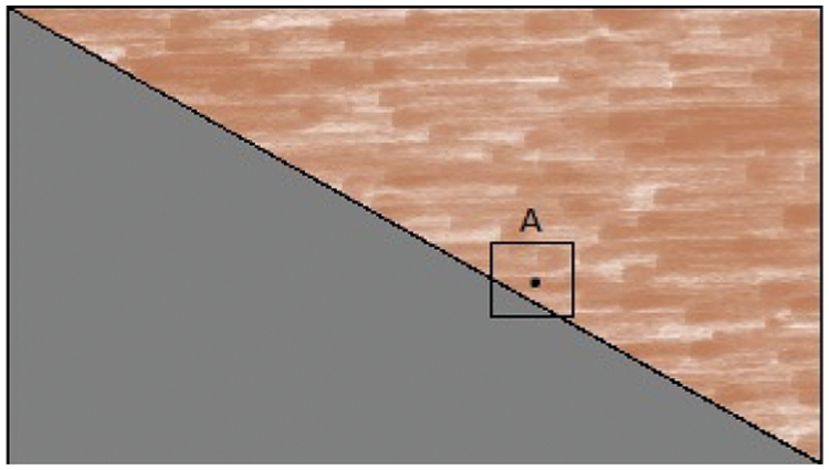
Figure 1: The local spectral histogram computed at location a within the square window
The above analysis is not valid in some scenarios: 1) An image window contains sub-regions that are too small to obtain meaningful histograms and 2) Filter scales are so large as to cause distorted histograms in near-boundary sub-regions, which makes it look different from the constant spectral histograms of the regions that include the sub-regions. However, these scenarios should have a minimal impact for the following reasons. For the first scenario, if a sub-region within a window is small, the contribution of this sub-region is little to the spectral histogram. Thus, it can be neglected in feature decomposition. However, a window could have many small sub-regions. For such scenarios applying this reason holds well. In a video, the background region remains the same or could slightly change in the case of dynamic background over several frames. Since our motivation is to capture the background statistics over many frames, the features of these small regions can be neglected during background estimation. For the second scenario, the purpose of filtering in a spectral histogram is to capture a meaningful pattern so the filters should not have large scales.
4 Proposed Background Estimation Algorithm
The most important part of any background subtraction algorithm is background modeling. In the case of traffic videos, constructing and maintaining a statistical representation of the scene that the camera sees is a fundamental task for background estimation. But, dynamic backgrounds such as camera oscillations, waving trees, water rippling, and illumination changes such as general and slow changes in background (climate change) make this task critical. Further, foreground objects moving faster are not problematic but foreground objects staying stationary for a long time and moving again is a problem and it is crucial for background modeling in surveillance systems. By considering all these challenges, we propose the novel background modeling algorithm based on local spectral histogram and multivariate linear regression model to produce the background of the video captured by a non-moving camera with high accuracy. The proposed method produces better results for videos captured in dynamic environments also.
The background is considered as a set of static objects (set of pixels) representing the same appearance over time. Due to foreground object movements, the intensity value of corresponding pixels changes over time. We assume that the pixel remains the same for the background and it changes for foreground objects over time. Under this consideration, we illustrate an idea by taking an example of a video sequence where only two objects are moving in the foreground. The evolution of a pixel at location p is represented in Fig. 2 over time. The pixel belonging to the background object remains approximately constant than the pixels belonging to the foreground object. Based on this idea, the proposed algorithm estimates the background of the video by taking into account just the feature vectors of pixels obtained from local spectral histograms through linear convolution of a bank of filters with a window centered at each pixel location over time. In this feature-based method, the representation of background value is determined by solving the linear regression problem modeled in Eq. (6), where,
Applying the change of variables Eq. (6) will be transformed into Y= Zβ +ɛ, where
where Y is an M × N matrix whose columns are feature vectors of all pixels at location p and time t, t+1,…., t+n. Next, Z is an M × 2 matrix whose columns are representative features, representing the constant background and foreground features at location p, β is 2 × N matrix whose columns are weight vectors and ɛ is an M × N matrix representing noise.
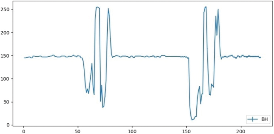
Figure 2: Gray level color changes
At each pixel location, two representative features have been defined, which should be approximately equal to the spectral histograms of background pixels and foreground pixels over time. By extending the above analysis, the features at a pixel location over time can be regarded as the linear combination of two representative features weighted by the corresponding area coverage of the image window. A multivariate linear regression model has been used to associate each feature to the representative features. When the feature matrix Y and the representative feature set Z are given,
Therefore, the background result is provided by examining
Now let
Certain constraints could be enforced on least-square solutions, such as the sum of the weight vector of each pixel should be equal to one and the weight vector should be non-negative. The algorithm for solving least square estimation and background modeling has been presented and the results are shown in Section 5. The values of n and λ are determined empirically. The chosen value are n= 200 and λ = 28. Fig. 3 shows spectral histograms of image windows centered at location p on five different video frames selected randomly. Image windows on frames 880, 914, and 959 give background histograms and that on frame 939 gives foreground histograms. Similarly, frame 942 gives mixtures of background and foreground histograms, due to the area covered by the image window consisting of both background and foreground regions. Finally, all the histograms are given as input to Algorithm 2 to estimate the representative features. As shown in Fig. 4, the spectral histograms of image windows and two representative features such as background and foreground features are given to Algorithm 1 for solving linear regression using the least-square method. Each pixel has been classified into either background or foreground based on the weight values of
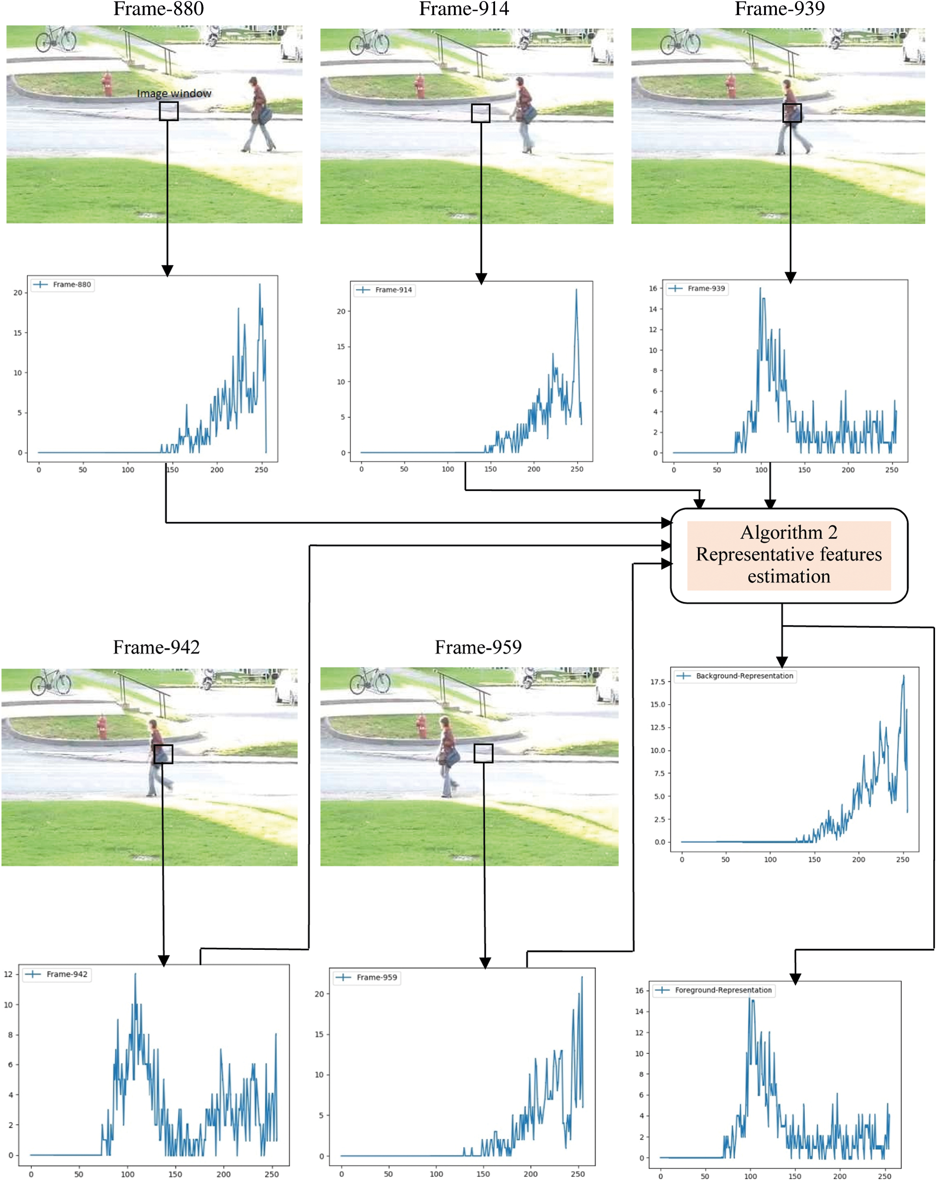
Figure 3: Local spectral histogram representation of image window and calculation of background and foreground representative features
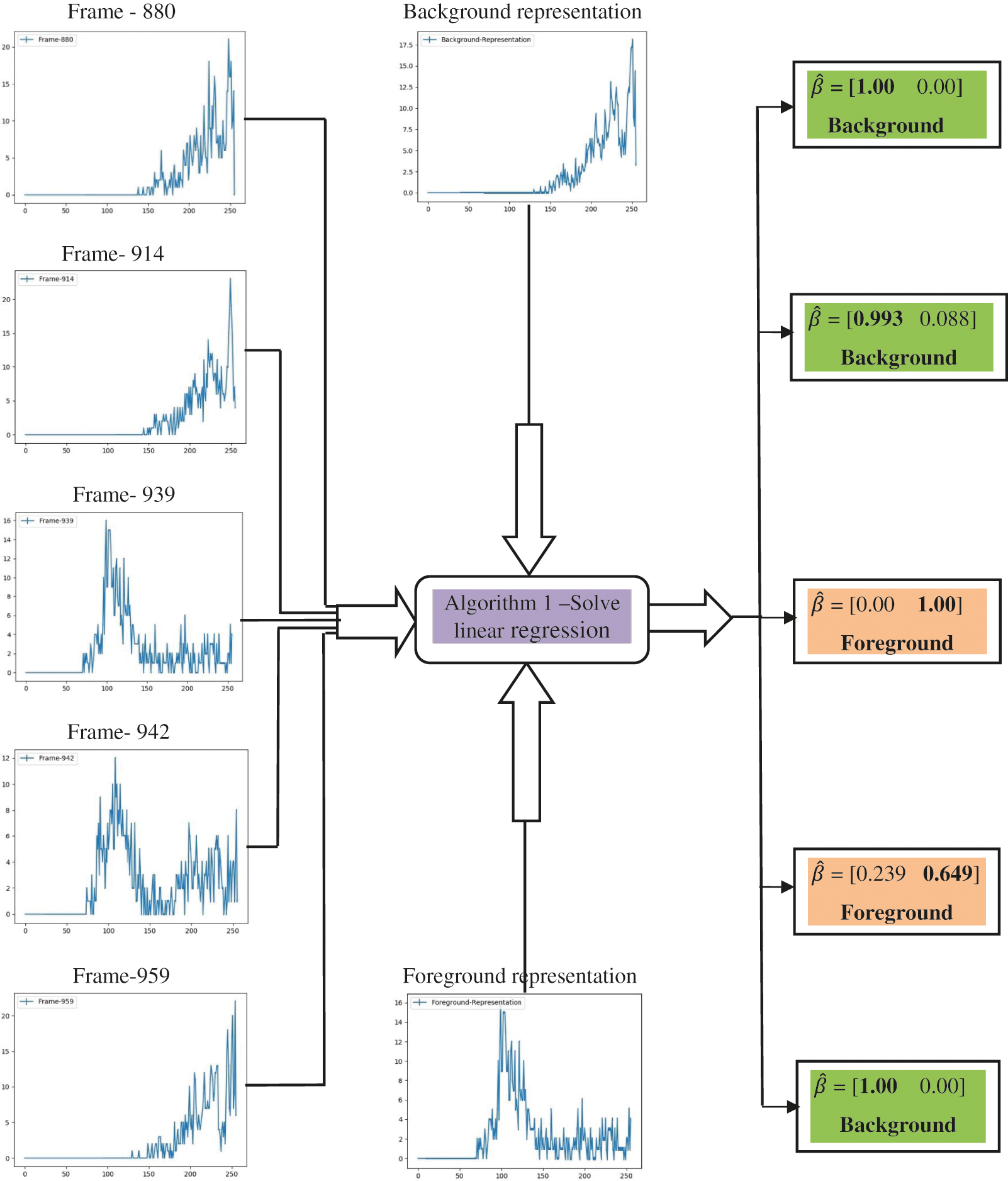
Figure 4: Estimation of weights through linear regression with representative features
4.2 Representative Feature Selections
In this section, an unsupervised method has been presented to obtain the background and foreground representative features which roughly represent background and foreground information. When comparing Xi and Xj, if the proximity is below the threshold Tp then no action is being performed. When a match occurs, the histogram Xj is added into the set Si. Similarly, all the histograms Xj where j = 1, 2, 3,….., t are compared, and the matched histograms are added to the set Si. The same operation is performed for all X0, X1,…..,Xt and sets S0, S1,……,St has been formed. The set with maximum size represents background histograms and the set with minimum size represents foreground histograms. Further, the K-means clustering algorithm is applied to these two sets, and the cluster centers are taken to represent background and foreground features. Fig. 5 shows the manually calculated background representative feature for a video frame taken inside the office (indoor video). The algorithm presented (Algorithm 2) has been applied on 10 video frames selected randomly from the same video and the results of this algorithm are shown in Fig. 6. The proximity threshold TP has been given as 0.6. For all our test sequences, the values of TP between 0.6 and 0.7 gave good results.
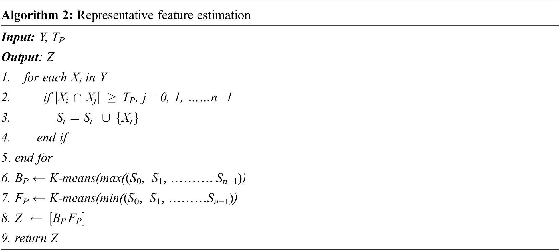
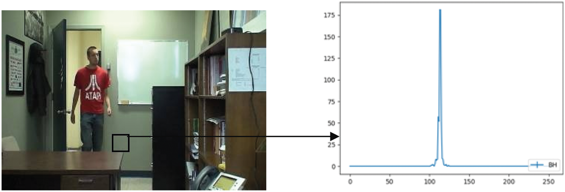
Figure 5: Manual calculation of background representative features over image window centered at p for indoor video
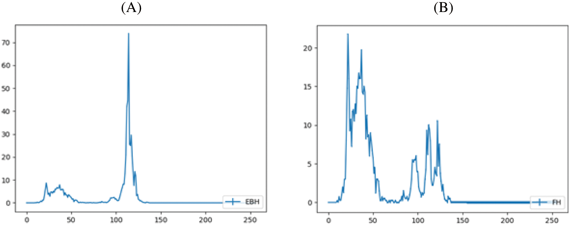
Figure 6: At location p, (A) Background representative feature calculated from algorithm 2; (B) Foreground representative feature calculated from Algorithm 2
5 Experimental Results and Analysis
5.1 Dataset and Performance Metrics
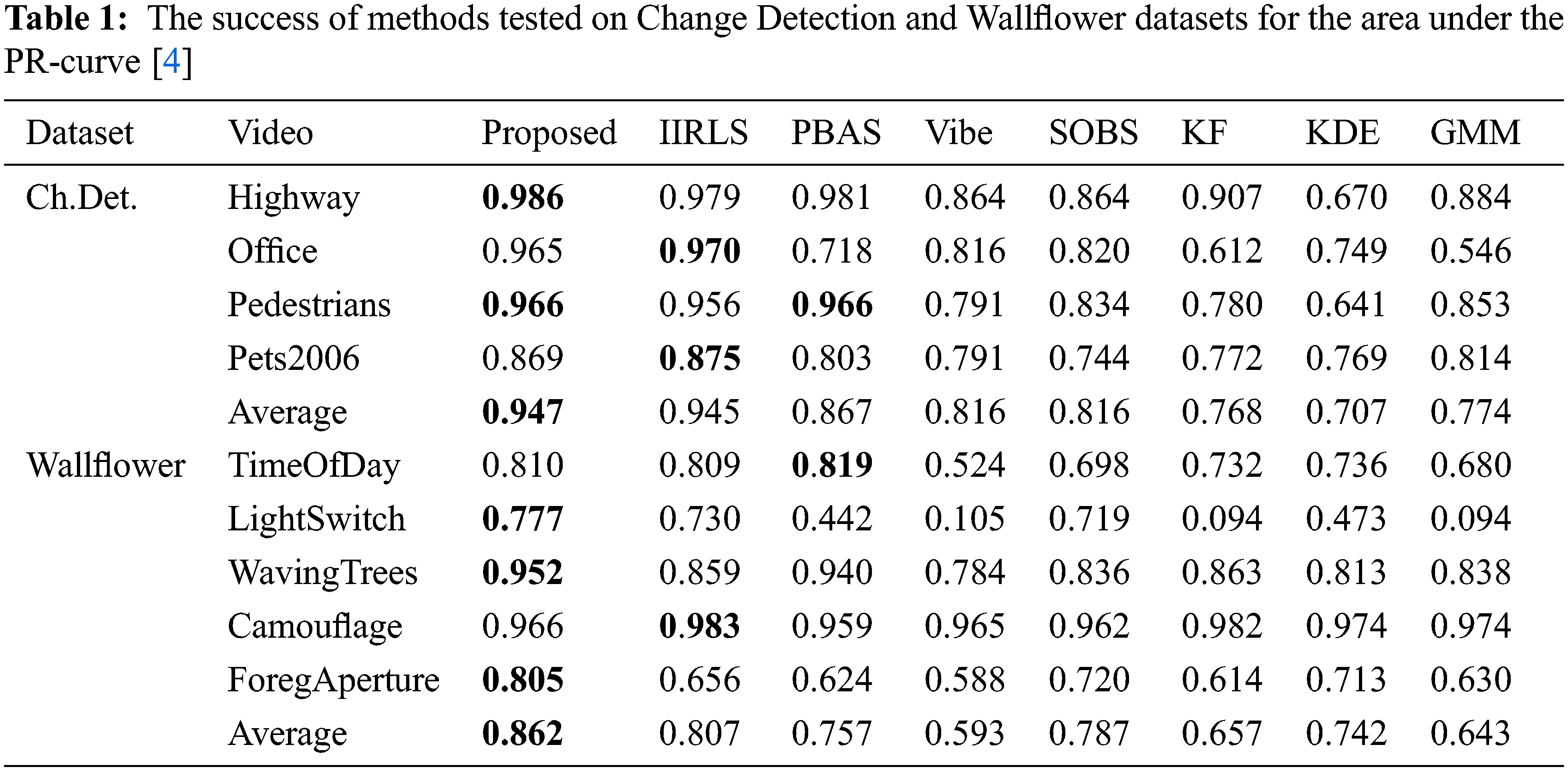
The well-known benchmark datasets for background subtraction include the Change Detection dataset (CDnet 2014) [33], the wallflower dataset [34], and the SBMI dataset [35]. Wallflower and SBMI datasets consist of both indoor and outdoor environments with an image resolution of 240 × 320 and 160 × 120. ChangeDetection.net dataset includes a wide range of detection challenges and typical indoor and outdoor scenarios. The dataset consists of videos that are classified into 11 categories. Since our method focuses on static cameras, we exclude the camera jitter (CJ) and Pantilt-Zoom camera (PTZ) categories. To test the performance of the proposed method, we selected one video sequence from each of the remaining categories.
The performance of the background estimation algorithms has been evaluated quantitatively by distributing the normalized absolute difference between the estimated results and the corresponding input images for both background and foreground regions. The Receiver Operating Characteristic (ROC) curve and the area under this curve are the most commonly used evaluation approaches, especially in medical image analysis [36]. The Precision-Recall curve (PR graph) gives more robust results in terms of performance [37] when the amount of data clustered in two classes is not uniformly distributed. Therefore, in this work the PR graph and the area under this curve are used to justify the efficiency of the proposed method based on TP (True Positive): the number of foreground pixels determined as foreground, FP (False Positive): the number of background pixels determined as foreground, FN (False Negative): the number of foreground pixels determined as background and TN (True Negative): the number background pixels determined as background. The PR graph has been generated by using the points computed from precision and recall values. Therefore, the area under the PR graph is calculated by integrating precision values over recall values. Tab. 1 shows the comparative results of the proposed method with the other existing methods. It is observed that the proposed method produces better results for most of the videos, particularly for videos with a dynamic background. Calculation of precision, recall, and area under the PR curve are as given below:
• RE (Recall) = TP / (TP + FN)
• PR (Precision) = TP / (TP + FP)
•
• F-measure(FM) = (2*Precision* Recall) / (Precision + Recall)
• Specificity (SP) = TN / (TN + FP)
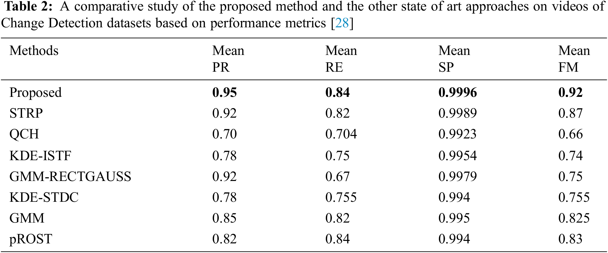
It is expected that PR, RE, SP, and F-measure must have higher values for any method to ensure higher accuracy in outcomes. Since the proposed method focuses on effective foreground extraction using combined spatial-texture features and a multivariate linear regression model, the accuracy obtained is higher than other existing methods. Tab. 2 shows the comparative results of the proposed method and other existing methods based on PR, RE, SP, and F-measure. It can be inferred that the proposed method outperforms the other existing methods.
5.2 Foreground Extraction in Change Detection Dataset
5.3 Background Estimation Results on SBMI Dataset
In Figs. 7 and 8, the results of our proposed method have been presented for the Change Detection dataset and SBMI dataset respectively. Also, the results are compared with corresponding Ground Truth (GT) images as well. The representative video frame of a whole video sequence, the estimated background, Ground truth, and the results obtained by our proposed method are shown in Fig. 7. The results of the proposed method compared with the corresponding GT of the SBMI dataset are also shown in Fig. 8.
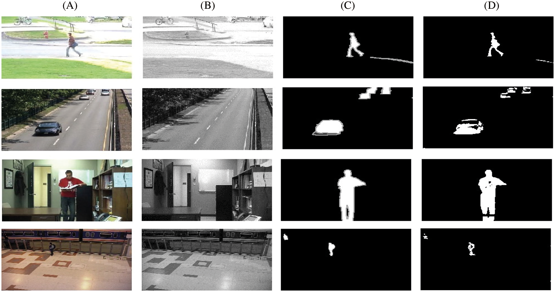
Figure 7: Experiment results: a) frame in the video sequence, b) modeled background, c) ground truth, d) our results
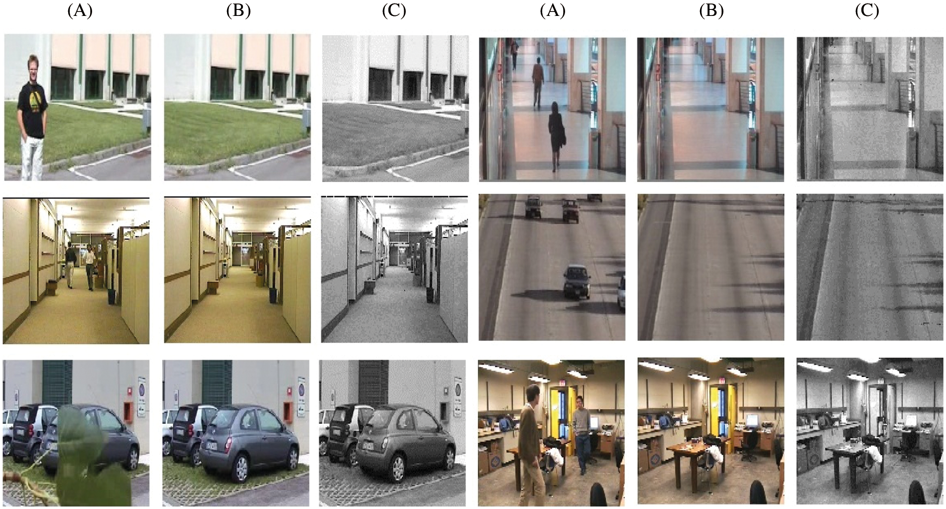
Figure 8: Experiment results: a) frame in the video sequence, b) ground truth, c) modeled background
In this paper, a dynamic background modeling technique has been presented using spectral-texture features. The features are extracted from a local spectral histogram which is used to estimate the background from the video. The modeled background is then used to detect and extract the foreground effectively. Due to the discriminative nature of the feature, the proposed method works robustly in challenging situations like dynamic background, ghosting effect, illumination variations, etc.
The proposed method has been evaluated against several video sequences including both indoor and outdoor scenes. The results have proven to be tolerant to illumination variations and the introduction or removal of background objects. We obtained the maximum value for PR, RE, SP, and FM is 0.98, 0.89, 1.00, and 0.97 respectively. Statistical measures have been included in this work to verify the efficiency of the proposed method. However, the method suffers from the limitations like shadow detection, misclassification due to sudden light changes, and camera oscillations. These could be the future scope to make this work more robust. Moreover, least-square estimation for each pixel and to find the background pixel corresponding to the maximum weight, this method has a high computational cost. Performing real-time applications with higher resolution images on a single processor machine would take more time. Usage of special hardware or multi-core graphics cards could make real-time applications possible with our proposed method.
Acknowledgement: The authors would like to thank the anonymous reviewers and editors for their valuable comments and suggestions.
Funding Statement: The authors received no specific funding for this study.
Conflicts of Interest: The authors declare that they do not have any financial or potential conflicts of interest.
1. L. Li, Z. Wang, Q. Hu and Y. Dong, “Adaptive nonconvex sparsity based background subtraction for intelligent video surveillance,” IEEE Transactions on Industrial Informatics, vol. 17, no. 6, pp. 4168–4178, 2020. [Google Scholar]
2. N. Buch, S. A. Velastin and J. Orwell, “A review of computer vision techniques for the analysis of urban traffic,” IEEE Transactions on Intelligent Transportation Systems, vol. 12, no. 3, pp. 920–939, 2011. [Google Scholar]
3. J. Yuan, D. L. Wang and R. Li, “Remote sensing image segmentation by combining spectral and texture features,” IEEE Transactions on Geosciences and Remote Sensing, vol. 52, no. 1, pp. 16–24, 2013. [Google Scholar]
4. M. Balcilar and A. Coskun Sonmez, “Background estimation method with incremental iterative Re-weighted least squares,” Signal, Image and Video Processing, vol. 10, no. 1, pp. 85–92, 2016. [Google Scholar]
5. J. Heikkila and O. Silvén, “A Real-time system for monitoring of cyclists and pedestrians,” in Proc. Second IEEE Workshop on Visual Surveillance (VS'99) (Cat. No. 98-89223), IEEE, pp. 74–81, 1999. [Google Scholar]
6. D. Koller, J. Weber, T. Huang, J. Malik and G. Ogasawara, “Towards robust automatic traffic scene analysis in real-time,” in Proc. of 12th Int. Conf. on Pattern Recognition, Lake Buena Vista, FL, USA, vol.1, pp. 126–131, 1994. [Google Scholar]
7. R. Cucchiara, C. Grana, M. Piccardi and A. Prati, “Detecting moving objects, ghosts, and shadows in video streams,” IEEE Transactions on Pattern Analysis and Machine Intelligence, vol. 25, no. 10, pp. 1337–1342, 2003. [Google Scholar]
8. C. R. Wren, A. Azarbayejani, T. Darrell and A. P. Pentland, “Pfinder: Real-time tracking of the human body,” IEEE Transactions on Pattern Analysis and Machine Intelligence, vol. 19, no. 7, pp. 780–785, 1997. [Google Scholar]
9. C. Stauffer and W. E. L. Grimson, “Learning patterns of activity using real-time tracking,” IEEE Transactions on Pattern Analysis and Machine Intelligence, vol. 22, no. 8, pp. 747–757, 2000. [Google Scholar]
10. Z. Zivkovic, “Improved adaptive Gaussian mixture model for background subtraction,” in Proc. of the 17th Int. Conf. on Pattern Recognition, ICPR, IEEE, Cambridge, UK, vol.2, pp. 28–31, 2004. [Google Scholar]
11. O. Tuzel, F. Porikli and P. Meer, “A Bayesian approach to background modeling,” in 2005 IEEE Computer Society Conf. on Computer Vision and Pattern Recognition (CVPR'05)-Workshops, San Diego, CA, USA, pp. 58–58, IEEE, 2005. [Google Scholar]
12. A. Elgammal, R. Duraiswami, D. Harwood and L. S. Davis, “Background and foreground modeling using nonparametric kernel density estimation for visual surveillance,” in Proc. of the IEEE, vol. 90, no.7, pp. 1151–1163, 2002. [Google Scholar]
13. O. Barnich and M. V. Droogenbroeck, “ViBe: A universal background subtraction algorithm for video sequences,” IEEE Transactions on Image Processing, vol. 20, no.6, pp. 1709–1724, 2010. [Google Scholar]
14. M. Hofmann, P. Tiefenbacher and G. Rigoll, “Background segmentation with feedback: The pixel-based adaptive segmenter,” in 2012 IEEE Computer Society Conf. on Computer Vision and Pattern Recognition Workshops, IEEE, Providence, RI, USA, pp. 38–43, 2012. [Google Scholar]
15. R. Chang, T. Gandhi and M. M. Trivedi, “Computer vision for multi-sensory structural health monitoring system,” in 7th IEEE Conf. on Intelligent Transportation Systems, Piscataway, NJ, 2004. [Google Scholar]
16. S. Messelodi, C. M. Modena and M. Zanin, “A computer vision system for the detection and classification of vehicles at urban road intersections,” Pattern Analysis and Applications, vol. 8, no. 1, pp. 17–31, 2005. [Google Scholar]
17. J. Zhong and Sclaroff, “Segmenting foreground objects from a dynamic textured background via a robust kalman filter,” in Proc. Ninth IEEE Int. Conf. on Computer Vision, IEEE, Nice, France, pp. 44–50, 2003. [Google Scholar]
18. D. Comaniciu and P. Meer, “Mean shift: A robust approach toward feature space analysis,” IEEE Transactions on Pattern Analysis and Machine Intelligence, vol. 24, no. 5, pp. 603–619, 2002. [Google Scholar]
19. J. Wu, J. Xia, J. Chen and Z. Cui, “Adaptive detection of moving vehicle based on on-line clustering,” Journal of Computers, vol. 6, no. 10, pp. 2045–2052, 2011. [Google Scholar]
20. M. Benalia and S. Ait-Aoudia, “An improved basic sequential clustering algorithm for background construction and motion detection,” in Int. Conf. Image Analysis and Recognition, Springer, Berlin, Heidelberg, pp. 216–223, 2012. [Google Scholar]
21. K. Kim, T. H. Chalidabhongse, D. Harwood and L. Davis, “Background modeling and subtraction by codebook construction,” in 2004 Int. Conf. on Image Processing, 2004. ICIP'04, IEEE, Singapore, vol.5, pp. 3061–3064, 2004. [Google Scholar]
22. H. Hu, L. Xu and H. Zhao, “A spherical codebook in YUV color space for moving object detection,” Sensor Letters, vol. 10, no. 1–2, pp. 177–189, 2012. [Google Scholar]
23. E. Goceri and N. Goceri, “Deep learning in medical image analysis: Recent advances and future trends,” in Int. Conf. on Computer Graphics, Visualization, Computer Vision and Image Processing, Lisbon, Portugal, pp. 305–311, 2017. [Google Scholar]
24. K. Lim, W. D. Jang and C. S. Kim, “Background subtraction using encoder-decoder structured convolutional neural network,” in 2017 14th IEEE Int. Conf. on Advanced Video and Signal Based Surveillance (AVSS), IEEE, pp. 1–6, 2017. [Google Scholar]
25. M. Heikkila, M. Pietikainen and J. Heikkila, “A Texture-based method for detecting moving objects,” in Bmvc, vol. 401, pp. 1–10, 2004. [Google Scholar]
26. T. Ojala, M. Pietikainen and T. Maenpaa, “Multiresolution gray-scale and rotation invariant texture classification with local binary patterns,” IEEE Transactions on Pattern Analysis and Machine Intelligence, vol. 24, no. 7, pp. 971–987, 2002. [Google Scholar]
27. M. Heikkila and M. Pietikainen, “A Texture-based method for modeling the background and detecting moving objects,” IEEE Transactions on Pattern Analysis and Machine Intelligence, vol. 28, no. 4, pp. 657–662, 2006. [Google Scholar]
28. S. Maity, A. Chakrabarti and D. Bhattacharjee, “Background modeling and foreground extraction in video data using spatio-temporal region persistence features,” Computers & Electrical Engineering, vol. 81, pp. 106520, 2020. [Google Scholar]
29. L. Maddalena and A. Petrosino, “A Self-organizing approach to background subtraction for visual surveillance applications,” IEEE Transactions on Image Processing, vol. 17, no. 7, pp. 1168–1177, 2008. [Google Scholar]
30. T. Bouwmans, “Recent advanced statistical background modeling for foreground detection-a systematic survey,” Recent Patents on Computer Science, vol. 4, no. 3, pp. 147–176, 2011. [Google Scholar]
31. T. Bouwmans and E. H. Zahzah, “Robust PCA via principal component pursuit: A review for a comparative evaluation in video surveillance,” Computer Vision and Image Understanding, vol. 122, pp. 22–34, 2014. [Google Scholar]
32. X. Liu and D. L. Wang, “A spectral histogram model for texton modeling and texture discrimination,” Vision Research, vol. 42, no. 23, pp. 2617–2634, 2002. [Google Scholar]
33. N. Goyette, P. M. Jodoin, F. Porikli, J. Konrad and P. Ishwar, “ChangeDetection. net: A new change detection benchmark dataset,” in 2012 IEEE Computer Society Conf. on Computer Vision and Pattern Recognition Workshops, IEEE, Providence, RI, USA, pp. 1–8, 2012. [Google Scholar]
34. K. Toyama, J. Krumm, B. Brumitt and B. Meyers, “Wallflower: Principles and practice of background maintenance,” in Proceedings of the Seventh IEEE International Conference on Computer Vision, IEEE, Kerkyra, Greece, vol. 1, pp. 255–261, 1999. [Google Scholar]
35. W. Wang, Y. Wang, Y. Wu, T. Lin and S. Li, “Quantification of full left ventricular metrics via deep regression learning with contour-guidance,” IEEE Access 7, pp. 47918–47928, 2019. [Google Scholar]
36. E. Goceri, Z. K. Shah and M. N. Gurcan, “Vessel segmentation from abdominal magnetic resonance images: Adaptive and reconstructive approach,” International Journal for Numerical Methods in Biomedical Engineering, vol. 33, no. 4, pp. e2811, 2017. [Google Scholar]
37. J. Davis and M. Goadrich, “The relationship between precision-recall and ROC curves,” in Proc. of the 23rd Int. Conf. on Machine Learning, Pittsburgh Pennsylvania USA, pp. 233–240, 2006. [Google Scholar]
 | This work is licensed under a Creative Commons Attribution 4.0 International License, which permits unrestricted use, distribution, and reproduction in any medium, provided the original work is properly cited. |