Intelligent Automation & Soft Computing DOI:10.32604/iasc.2022.023717
Article

Adaptive Fuzzy Robust Tracking Control Using Human Electromyogram Signals for Elastic Joint Robots

Mahdi Souzanchi-K1, Mohammad-R Akbarzadeh-T1,*, Nadia Naghavi1, Ali Sharifnezhad2 and Vahab Khoshdel3

1Department of Electrical Engineering, Center of Excellence on Soft Computing and Intelligent Information Processing, Ferdowsi University of Mashhad, Mashhad, Iran
2Sport Science Research Institute of Iran (SSRII), Tehran, Iran
3Department of Mechanical Engineering, Center of Excellence on Soft Computing and Intelligent Information Processing, Ferdowsi University of Mashhad, Mashhad, Iran
*Corresponding Author: Mohammad-R Akbarzadeh-T. Email: akbazar@um.ac.ir
Received: 18 August 2021; Accepted: 09 November 2021

Abstract: Sliding mode control is often used for systems with parametric uncertainties due to its desirable robustness and stability, but this approach carries undesirable chattering. Similarly, joint elasticity is a common phenomenon induced by transmission systems in robots, but it presents additional complexity in robot dynamics that could lead to robot vibrations or even instability. Coupling these two phenomena presents further compounded challenges, particularly when faced with the human interface's added uncertainties. Here, a stable voltage-based adaptive fuzzy strategy to sliding mode control is proposed for an elastic joint robot arm that uses a human's upper limb electromyogram (EMG) signals to direct its movement. The concurrent use of EMG with the elastic joint arm provides a suitable framework for human-robot interaction. EMG signals represent human's ‘intention’ on motion, i.e., they move between 50–100 ms before the mechanical motion begins. Hence this strategy potentially builds better synchronization between the robot and human intention. Furthermore, the adaptive fuzzy strategy eliminates the system chattering while also providing robustness against parametric uncertainties and time delay. Lyapunov analysis also shows bounded-input bounded-output stability of the closed-loop system. Finally, the proposed approach is experimentally implemented in the Sport Science Research Institute. Comparisons with a competing strategy, as well as a torque mode controller, shows that the proposed approach leads to a computationally faster and more accurate controller.

Keywords: Adaptive fuzzy control; artificial neural network; elastic joint robot; electromyogram signal; sliding mode control; voltage control strategy

1  Introduction

It is increasingly clear that robots will fulfill a growing number and range of duties in modern life. Human-robot interaction and its various applications have hence received considerable attention in the past several years. However, the complexity of sensing processes and dynamics of biological systems, coupled with nonlinearities of robot dynamics, have considerably challenged every successful experimental development. In particular, there is a fundamental shortage of study in developing a system of sensors to conveniently map human desires and intentions to the robot's actions.

Recent studies differ considerably in their approach to human-robot interaction. For example, a robust nonlinear scheme is introduced in [1,2] explains the multi-user human-robot interaction, Mixed Integer Programming (MIP) model is used for evaluating navigation and task planning [3], some rehabilitation application is used in [4,5] explains hierarchical learning in human-robot interaction. A novel notion is proposed using surface electromyography (EMG) signals as a human-sensory interface for such isokinetic motion control purposes. The isokinetic exercise is of great importance here since natural motion in telesurgery and physiotherapy applications favor robots that move slowly with high accuracy. When a user naturally moves his/her arm, the corresponding muscle activation is measured through the EMG signals and mapped against environmental kinematic information. For example, estimation of upper limb joint angle [6], finger reflexes on a robotic hand [7], hand model based on the classification of individual finger movements [8], and finger joint angles position [9] are shown this issue. These signals provide valuable information on the user's intention to move between 50–100 ms before the motion actually occurs [10]. Such early detection is an invaluable asset in applications with naturally occurring time delays, such as robot teleoperation in surgical applications.

An essential aspect of our interface relies on the fact that the EMG signals can be recorded for almost everyone, even those with limb amputations since EMG can be recorded merely by placing the surface electrodes on the participant's skin. While the EMG signals and arm motions are related in a very complex and highly nonlinear manner [11], they are already used in some applications such as the directional control of rehabilitation robots [12], control of multi-fingered robot hands [13], and human-assistive manipulators [14].

The above works assume robot rigidity. They also often ignore the dynamics of the employed electrical actuators and expect a power transmission system coupled with the electrical motors, by which high torques can be generated at relatively low speeds. This is while joint elasticities are a common phenomenon induced by transmission system deformations. This is particularly unreasonable for the small size and subtle movements in applications such as telesurgery. However, with elastic joint robots, the link angle no longer follows the actuator angle, hence doubling the robot's degrees of freedom (states) compared to the number of control actions. Thus, joint elasticity presents additional complexity and nonlinearity through its input-output coupling and, as indicated in [15], is the primary source of robot vibrations or even instability. Accordingly, elastic joint robots present a formidable challenge, especially in applications with high precision requirements.

Much research has addressed elastic joint robots’ modeling and control. For instance, an efficient finite element formulation is introduced for robot modeling [16]. In the robot control area, neural network control [17], tip control [18], proxy-based position control [19], and force-free control [20] are provided. These methods are based on the torque control strategy, a common approach for robot control [21–23]. However, such controllers carry high computational complexity due to manipulator dynamics that are more complicated in elastic arms. Furthermore, these strategies often ignore the actuator dynamics. This is while less computation and simple actuator dynamics are vital for successful high precision control of elastic arms.

Here we use a voltage control strategy that is free from robot dynamics [24]. This view takes the challenge from robot dynamic control to actuator control, so the controller design is simplified. There are some theories based on this strategy, such as adaptive fuzzy control [25], robust control [26], impedance control [27], and adaptive control [28]. Souzanchi-K et al. [29] also used this general strategy in a human-robot interaction application in which a Multi-Layer Perceptron (MLP) is pre-trained to match EMG signals to the kinematic data of a human hand's movement. However, their voltage-based controller requires the exact actuator dynamics, which may either be unavailable or change in time.

In contrast with [29], here, we aim for a robust adaptive control strategy. Accordingly, we propose a voltage-controlled Adaptive Fuzzy Sliding Mode Controller (AFSMC) for elastic joint robot arms guided by EMG signals. The closed-loop system's stability is guaranteed following a Lyapunov analysis of the sliding mode framework, despite the high model complexities, parameter uncertainty, and noisy measurements. Compared to [29], results show that the proposed strategy is more robust against uncertainties such as random time delay and un-modeled dynamics.

The above qualities have already been confirmed for sliding-based designs in several reports such as [30–33], but sliding-based approaches also carry undesirable chattering when the system operates near the sliding surface. This chattering, in turn, agitates the un-modeled high ordered nonlinear dynamics. Hence, an adaptive fuzzy strategy is considered here that provides a smoother control effort to eliminate the chattering effect. Finally, the proposed AFSMC directly controls the joint angles via one control loop, compared with the two control loops that are typical in most of the earlier controllers for elastic joint robots.

The proposed control strategy is also compared with the control strategy [34]. This strategy is torque (current)-based, uses forward and inverse kinematics, and ignores the dynamics of their electric actuators and joint elasticity. To have a fair comparison, this strategy is simulated on the robot of this study.

The remainder of this paper is organized as follows. The proposed control architecture, robot modeling, theoretical analysis of stability, and results from experimental implementation at the Sports Science Research Institute are discussed in Section 2. Section 3 offers conclusions and further discussions on future works.

2  Methodology

Here, we describe the training and real-time laboratory procedures to control the proposed elastic joint robot arm using surface EMG. We consider the upper limb muscles to focus on the future utility of the approach in telesurgery. In the primary stage, the participant is advised to move his/her arm in random patterns. During this movement, a Cortex motion capture system records the arm movement trajectory, while the EMG electrodes record the activities of four muscles from the shoulder and elbow. The processed signals are then used to train an Artificial Neural Network (ANN) model that estimates arm movement trajectory in a real-time operation using only the EMG recordings. Upon the completion of the training phase, the real-time operation phase begins. In this phase, the participant controls the robot by using the AFSMC, directly by moving his or her hand.

2.1 Training Phase

2.1.1 Setup and EMG Data Collection

Four EMG channels are employed as principle input signals to assess the participant's arm movement trajectory, with each channel corresponding to one muscle, as depicted in Fig. 1. In our experiment, using an electrolytic gel interface, eight sticky surface electrodes (Ag/AgCl) are positioned above the muscle (with 2 cm inter-electrode distance) of the Biceps brachii, Triceps brachii (Long head), Deltoideus Medius, and Pectoralis major. Moreover, reference electrodes are placed on the elbow, Acromion, and Clavicle bony side. The skin on the exposed area is attentively shaved and cleaned with alcohol to minimize the impedance. To minimize the electrodes’ motion artifacts, they are excessively taped with the preamplifier to the skin with an elastic tape.

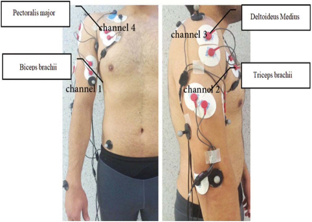
Figure 1: EMG electrodes placed on the user body

Several tests are performed to study the signal quality of each muscle. The device employed to record the EMG signal from muscles is ME6000 (BIOMATION Co., Almonte, Ontario, Canada, https://www.biomation.com). This device's data is sampled at 2 kHz, and the delay of EMG recording for this device is 3 ms. Six infrared cameras (Cortex) are used to track the participant's arm to record the trajectories in the plane coordinate. The cameras were calibrated before recording and trajectory post-processing is done by Cortex software. There appears a gap between these signals since the human trajectory and EMG signals are recorded separately with different devices. To fill the marker trajectory gaps and analyze data, the SIMM-Calcium skeleton, developed by Musculo Graphics (the creators of SIMM) and an enhanced Helen Hayes model, a popular marker set for built-in full-body models, are used.

2.1.2 Trajectory Estimation

The experiment was conducted using four male subjects, 25 to 30 years of age, who had never used EMG-controlled devices. During the training phase, the users were instructed to move their elbow and shoulder to random positions (with 2 degrees-of-freedom planar movements) 50 times to cover a wide range of the arm workspace. Hence, our training data consists of 160 instances, and the testing data set has 40 instances with the same number of inputs and outputs.

The desired robot trajectories are prepared using the estimated paths from processed EMG signals. The raw EMG signals are first normalized. Subsequently, the following three steps are performed. The first step is filtering the raw EMG signals by a 5th order notch filter to remove the 50 Hz power supply noise. The second step is to rectify the EMG signals, and the third step is calculating the signals’ Online Moving Average (OMA). The processed signal is written as,

E¯chi(t)=1N∑j=0N⁡E(t−j)2, (1)

where E¯chi(t) is the processed signal of EMG for each channel, N is the number of segments (N = 100) and E(t) is the value of the filtered and rectified EMG signals at its sampling point. Finally, the processed EMG signals shown in Fig. 2 are used as input to the ANN estimator. The ANN has 3 three layers: an input layer, a tan-sigmoid hidden layer, and a linear output layer.

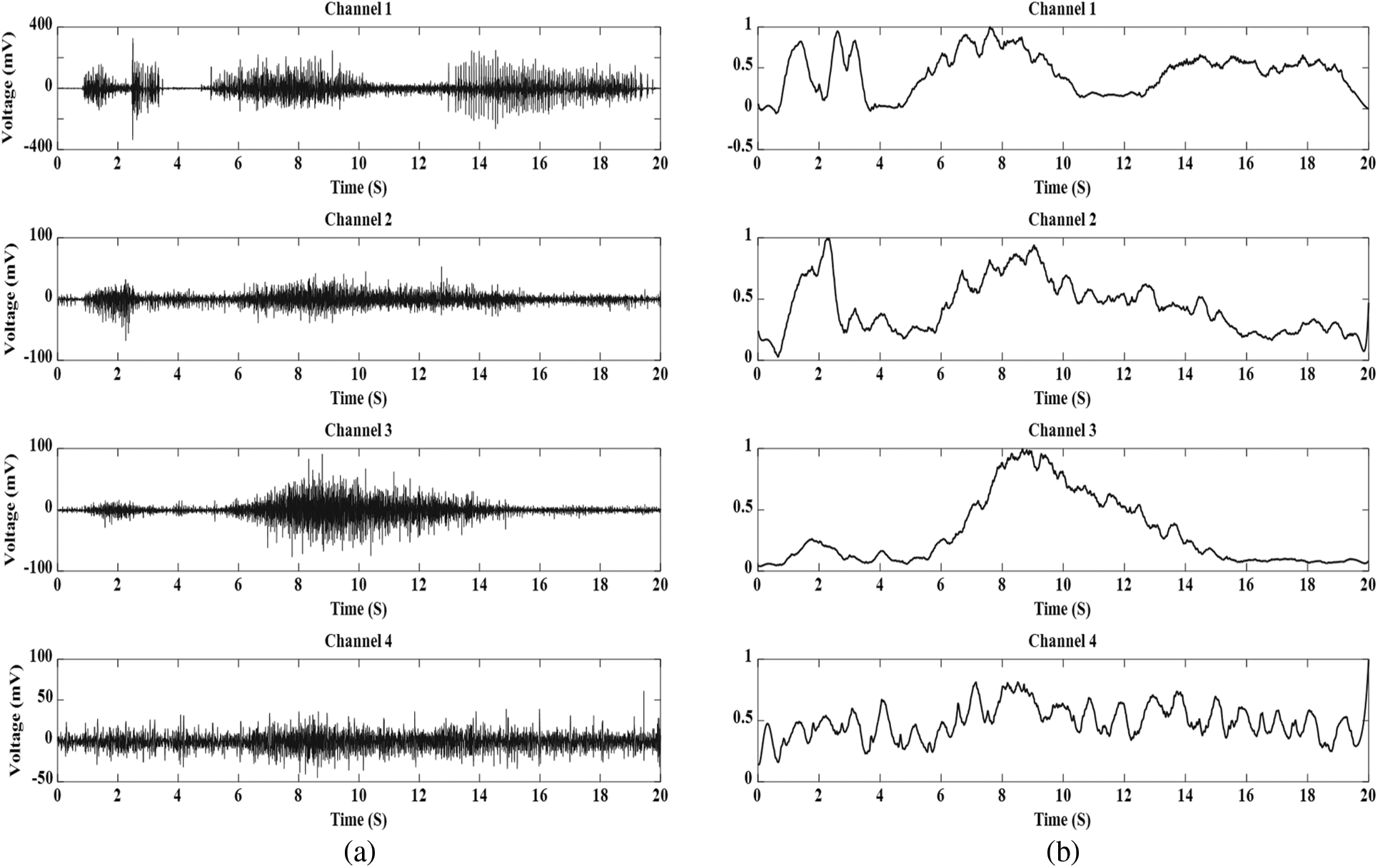
Figure 2: (a) Raw EMG signals. (b) Processed EMG signals for the input of the artificial neural network

Selecting the number of neurons in the hidden layer is still challenging since many hidden neurons may deteriorate the network performance and complicate the training process. Also, a large number of network variables require a large amount of memory. Networks with too few neurons in the hidden layer are also unable to properly adjust weights and biases during the training process, leading to overfitting and excessively complicating the training process. Here, the performance criteria for different ANN architectures are analyzed to determine the appropriate number of neurons. According to [35], the optimum ANN is specified with four input nodes, eight tan-sigmoid neurons in the hidden layer, and seven linear neurons in the output layer. Following the ANN design with the specified architecture and different hidden neurons, a suitable and efficient back-propagation training algorithm must adjust synaptic weights and biases at different layers.

The relationship between EMG channels and the participant trajectory is modeled as,

θhest=[E¯ch1(t)E¯ch2(t)E¯ch3(t)E¯ch4(t)]TW4×nhl1Wn×mhl2Wm×2ol, (2)

where θhest is hand's joint angle vector, E¯chi(t) is the processed signal of EMG for each channel, W4×nhl1 and Wn×mhl2 are the weight matrices related to hidden layers of the neural network and Wm×2ol is the weight matrix related to the output layer. It is necessary to mention that the duration of the training process was 180 s.

2.2 Real-Time Operation Phase

2.2.1 Robot Modeling

An integrated state-space model is introduced here using the robot kinematics and dynamics, including those of the actuator. By employing a linear torsional spring to represent the joint elasticity, the mechanical dynamics of the robot are illustrated as,

D(q)q¨+C(q,q˙)q˙+G(q)=K(rθm−q), (3)

Jθ¨m+Bθ˙m+rK(rθm−q)=τm, (4)

where θm ∈ Rn and q ∈ Rn are vectors of motor angles and joint angles, respectively. Hence, this framework has 2n coordinates indicated as [q, θm]. Also, D(q)∈Rn×n is the inertia matrix of the manipulator, C(q,q˙)q˙∈Rn is the vector of centrifugal and Coriolis forces, G(q) ∈ Rn is the vector of gravitational forces, and τm∈Rn  is the vector of motor torques. J, B, and r ∈ Rn×n are diagonal matrices representing motor inertia, motor damping, and reduction gear coefficients, respectively. K is the matrix of the joint and reduction gear's lumped elasticity. Moreover, the joint stiffness and gear coefficients are assumed to be constant. The gravitational force vector G(q) is considered to be a function of joint positions as part of a streamlined model [36]. The dynamical equations and parameters of D(q), C(q,q˙)andG(q) for robot modeling are mentioned in Appendix A.

Control of elastic joint robots is generally tricky since they are highly nonlinear, computationally costly, vigorously coupled, with double the size of the state space, i.e., 2n coordinates. Improved performance is expected if the proposed model is more accurate by including actuator dynamics. Consequently, we consider the electrical equations of DC motors with the motor voltages as inputs, as follows,

RaIa+LaI˙a+Kbθ˙m=V, (5)

where V ∈ Rn is the motor voltages vector, Ia ∈ Rn is the motor currents vector, and θ˙m is the vector of motor velocities. Also, Ra, La, Kb ∈ Rn×n are diagonal matrices representing the coefficients for armature resistance, armature inductance, and back-emf constant, respectively. The vector of torques τm is then derived as input for (4) using the motor currents vector as follows,

τm=KmIa, (6)

where Km  is a diagonal matrix representing the torque constants.

Eqs. (3)–(6) then form the robot dynamics, such that the input vector is the voltage vector V and the output vector is the joint angle vector q . Utilizing (3)–(6), the electrically driven elastic joint robot state-space model can be derived as,

X˙=f(X)+bV, (7)

f(X)=[X2D−1(X1)(−G(X1)−KX1−C(X1,X2)X2+KrX3)X4J−1(rKX1−r2KX3−BX4+−L−1(KbX4+RX5)KmX5)]

b=[0000L−1]X=[qq˙θmθ˙mIa]. (8)

Eq. (8) is a coupled, nonlinear multivariable system. The model complexity is a severe challenge in pieces of literature on elastic joint robot modeling and control.

A decentralized controller based on voltage strategy is proposed here for the real-time operation phase. Using (5), the mathematical equation for each electric motor is,

RIa+LI˙a+Kbθ˙m=V (9)

to indicate the joint velocity, (9) can be represented as,

q˙−q˙+RIa+LI˙a+Kbθ˙m=V. (10)

The system (10) is re-expressed as,

q˙+F=V, (11)

where the function F is expressed as,

F=RIa+LI˙a+Kbθ˙m−q˙. (12)

2.2.2 Sliding Mode Controller Based on Voltage Control Strategy

To design a novel sliding mode control law, the sliding surface should be defined as,

S=e+λ∫⁡edt. (13)

where e is the tracking error,

e=qd−q. (14)

In (13) and (14), qd and q, are the desired and actual joint angles, respectively, while λ is positive and constant-coefficient.

To obtain the proposed sliding mode control law, a positive definite function Λ is defined as,

Λ=12S2. (15)

A derivative of the above positive definite function with respect to time is then calculated as,

Λ˙=SS˙. (16)

For S → 0, it is sufficient that Λ˙<0 . So, let

SS˙=−α|S|, (17)

S˙sgn(S)=−α, (18)

where α is a constant and positive coefficient and sgn(S) = S/|S|. S˙ is calculated using (13) and substituting into (18) yields,

(e˙+λe)sgn(S)=−α. (19)

By substituting (11)–(19),

(q˙d+F−V+λe)sgn(S)=−α, (20)

where F is expressed by

F=F¯+ΔF, (21)

F¯=−q˙, (22)

ΔF=RIa+LI˙a+Kbθ˙m. (23)

However, the effect of LI˙a may be ignored [37] since the DC motor electrical time constant is considerably smaller than its mechanical time constant. Moreover, since I˙a might be prone to noise, measuring I˙a is not recommended. Hence,

ΔF≈RIa+Kbθ˙m, (24)

(q˙d+F¯−V+λe)sgn(S)=−α−ΔFsgn(S), (25)

−α−ΔFsgn(S)=η. (26)

By multiplying both sides of (25) in sgn(S), the control law V is calculated as,

V=q˙d+F¯+λe−ηsgn(S). (27)

It is well known that classical sliding mode control carries undesirable chattering due to the constant value of η and discrete function sgn(S). As a remedy, it is suggested to use saturation function sat(S∅) instead of sgn(S) to overcome this problem [38]. However, this approach introduces steady-state error to the sliding surface. Therefore, an adaptive fuzzy system is designed based on the sliding surface that estimates the control law.

2.2.3 Designing the Adaptive Fuzzy Controller Based on the Sliding Surface

We develop here a decentralized fuzzy controller using two variables, namely x1 and x2, as inputs to the controller, which are defined as,

x1=S=e+λ∫⁡edt, (28)

x2=S˙=e˙+λe. (29)

The motor voltage V is the controller output.

Three membership functions, P, Z, and N, are assigned to each fuzzy input x1 and x2; therefore, control input space is covered by nine fuzzy rules. These rules are proposed in the form of Mamdani type, as,

Rule l:If x1is Aland x2is Bl,then Vis Cl, (30)

where Rule l with l=1,…,9 , denotes the l th fuzzy rule. In the l th rule, Al, Bl, and Cl are fuzzy membership functions for variables x1, x2 and V, respectively. However, since the precise information on the ranges of x1 and x2 are not provided, S shape and Z shape membership functions are employed for P and N, respectively. These three functions are expressed as,

μZ(x1)=exp⁡(−x122σ2)σ=0.3. (31)

The membership functions for x2 are similar to those of x1.

The membership functions for the output V in Gaussian shapes are expressed as,

μCl(V)=exp(−(V−y^l)22σ2), (32)

where y^l is the center of Cl . To determine V, Mamdani inference engine, singleton fuzzifier and center average defuzzifier, along with (30)–(32), are used [39]. In other words,

V=∑l=19⁡y^lψl(x1,x2)=y^Tψ(x1,x2), (33)

where ψl is a fuzzy basis, which is a positive value expressed as,

ψl(x1,x2)=μAl(x1)μBl(x2)∑l=19⁡μAl(x1)μBl(x2), (34)

for μAl,μBl∈[0,1] , ψ = [ψ1…ψ9] T, and y^=[y^1…y^9]T is determined here using an adaptation law.

Applying the fuzzy control Eq. (33) to the system (27) leads to the below closed-loop system.

q˙d+F¯+λe−ηsgn(S)=y^Tψ(x1,x2), (35)

where y^ is the estimate of y, which is employed in a fuzzy system yTψ(x1, x2) to approximate the following function, according to the universal approximation theorem of fuzzy systems, that is,

e¨+k1e˙+k2e+q˙d+F¯+λe−ηsgn(S)=yTψ(x1,x2)+ϵ, (36)

where ɛ is the approximation error. Also, k1 and k2 are positive gains that are selected as control design parameters.

To derive the adaptation law, the tracking system is formed from (35) and (36), as below,

e¨+k1e˙+k2e=(y−y^)Tψ(x1,x2)+ϵ. (37)

The state-space equation is then obtained by using (37),

Z˙=AZ+Bw, (38)

where A=[0−k21−k1],B=[01],Z=[ee˙], and

w=(y−y^)Tψ(x1,x2)+ϵ. (39)

Here, a positive definite function H is suggested in the form of,

H=12ZTPZ+12α(yT−y^T)(y−y^), (40)

where the unique, symmetric, positive definite constants α > 0, and matrices P > 0 and Q > 0 satisfy the following Lyapunov equation,

ATP+PA=−Q, (41)

then, H˙ is calculated using (38)–(41) as,

H˙−12ZTQZ+ZTP2((yT−y^T) ψ(x1, x2)+ϵ)−1α(yT−  y^T)y^˙,(42)

where P2 denotes the second column of the matrix P. Thus, (42) is represented as,

H˙=−12ZTQZ+(yT−y^T)(ZTP2 ψ(x1, x2)−1αy^˙)+ZTP2ϵ.(43)

If the adaptive law is given by,

y˙^=αZTP2ψ(x1,x2). (44)

So we have,

y^=α∫0t⁡ZTP2ψ(x1,x2)dt+y^(0), (45)

where y^(0) is the initial value, and

H˙=−12ZTQZ+ZTP2ϵ. (46)

The tracking error is reduced if H˙<0 . To satisfy this condition, we should have,

ZTP2ϵ<12ZTQZ. (47)

One can imply λmin(Q) ||Z||2 < ZTQZ < λmax(Q) ||Z||2 where λmin(Q) and λmax(Q) are the minimum and maximum eigenvalues of Q, respectively. Hence, to satisfy the tracking error reduction condition H˙<0 it is sufficient to have,

2P2|ϵ|λmin(Q)<∥Z∥. (48)

2.3 Stability Analysis

In the following section, stability analysis for the closed-loop control system (35) is presented. The following assumptions are essential to make the tracking error dynamics well defined and to enable the robot to track the desired trajectory.

Assumption 1: The desired trajectory qd should be smooth enough in the sense that qd and its derivatives, up to necessary orders, are available and are all uniformly bounded [40].

Assumption 2: The electric motor should be protected against overvoltage. Hence, its voltage is bounded by a maximum value, as stated by |V| < Vmax.

Theorem 1: By meeting the requirements stated in Assumption 1, the variables e, e˙ , q, and q˙ remain bounded for the tracking system (37).

Proof: Eq. (38) is presented in a linear state-space. Now, if the eigenvalues of the matrix A are all negative because all real values are negative as well, then it can be said that the system is stable. Solving (38), which could be expressed as:

Zi=Zi(0)eAit+1Ai∫0T⁡(Bw)eA(T−t)dt. (49)

It can be said that the value of Bw is bounded since the operating time and estimation error are bounded. Hence, the integral of a bounded value in a bounded time is also bounded. On the other hand, the Zi(0) is bounded. Therefore the value of Zi converge to a negligible value, and the matrix Z is bounded.

Based on the Routh-Hurwitz criterion, the system in (38), a linear first-order system, is stable. Therefore, since Z and Bw are bounded, Z˙ is bounded as well.

Moreover, since in Assumption 1, it is assumed that the desired trajectory qd and its derivatives q˙d are bounded and since q = qd − e and q˙=q˙d−e˙ , then the boundedness of e and e˙ also implies that q and q are bounded, respectively.▪

Theorem 2: By considering Assumption 2 and the control law (27), Ia and θ˙m are bounded.

Proof: Assumption 2 indicates that V is bounded, according to (27) and Theorem 1, η is bounded. Eq. (26) shows the ΔF is bounded since η is bounded. Therefore, since ΔF is bounded, Ia and θ˙m are bounded. ▪

Theorem 3: By considering the dynamic equation of actuator and the boundedness of q, Ia and θ˙m , θm is bounded.

Proof: According to Theorems 1&2, the state vectors q, Ia and θ˙m are bounded. Substituting τm in (2) with (4) yields,

Jθ¨m+Bθ˙m+r2Kθm=KmIa+rKq. (50)

Since J, B and r2K are positive diagonal matrices, (50) is stable with the bounded input KmIa + rKq. As a result, the output θm is bounded. ▪

In conclusion, as the above theorems indicate, all system states are bounded. Thus, it is concluded that the proposed controller guarantees BIBO stability.

2.4 Results

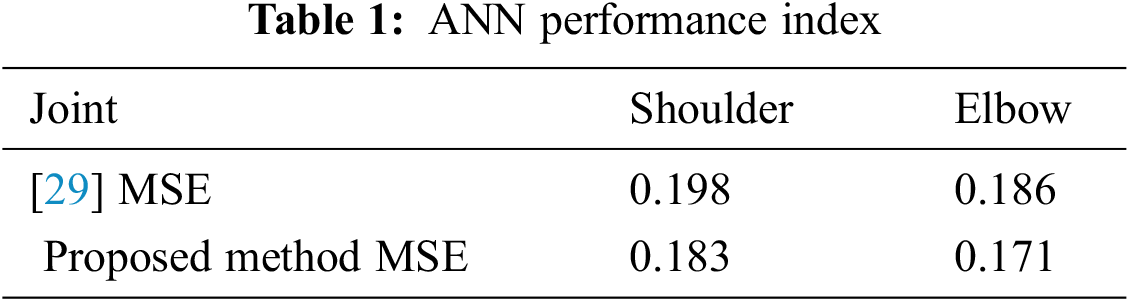
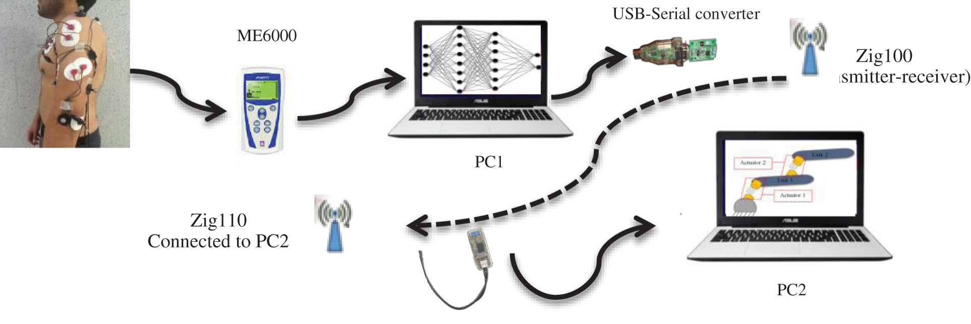
The experimental results are reported here in two phases. The first phase is about training an ANN to discover a mapping between EMG signals and the hand motion and the second phase is about the applying the proposed adaptive controller in a real-time operation. The Mean Squared Error (MSE) is used as a performance index for the ANN and Tab. 1 shows the effectiveness of the proposed method in the training phase. In the second phase, the performance of AFSMC is assessed via remote teleoperation of the elastic joint robot arm with EMG signals. In this experiment, two computers are employed. The computers used for the assessment are an Intel Core-i5, 2.60 GHz CPU with 8 gigabytes of RAM. One computer simulates the robot control system with MATLAB Simulation Toolbox, while the other acquires the EMG signals during the real-time operation phase. A wireless Zig-Bee radio module from Robotic Company (ZIG-110A), operating in 2.4 GHz frequency, connects the two computers with the serial protocol at 38400 bps rate. This experimental setup is shown in Appendix B.

The EMG signals provide information on the user's intention to move before the motion occurs; therefore, the trajectory is estimated before the participant moves his/her hand. This prediction should create added robustness in applications with communication delay, such as in telesurgery. To study this, we consider a uniform probability distribution function by using MATLAB (rand) function as a random time delay between 0–80 ms in this communication system. The proposed control law (33) is applied to each elastic joint robot arm's DC motor. To consider the parametric uncertainty, it is assumed that robot model parameters are about 0.8 of their actual values as provided in Tab. 2. Fig. 3 illustrates the proposed control system block diagram. In general, the control method is decentralized. During the real-time operation phase, the fifth participant moves his arm randomly. The desired trajectories are estimated in Computer 1 using the ANN and sent to Computer 2 for robot controlling.

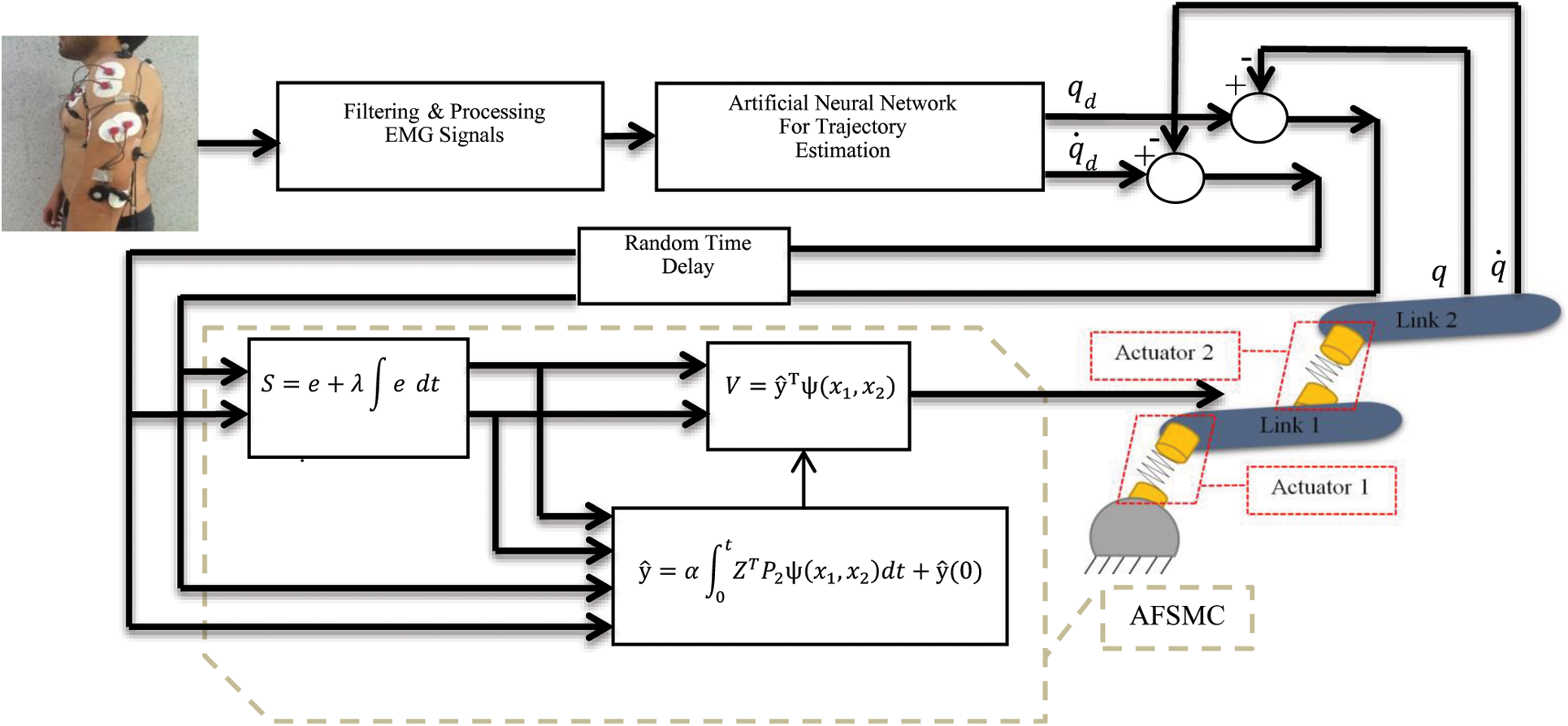
Figure 3: Block diagram of the proposed controller with random time delay

Some statistical results, such as the maximum error of each joint and MSE, are used as a performance index to evaluate the proposed method. Since the random time delay is used in communication channels, the experiment is run ten times, and Tab. 3 provides the average and the standard division of these performance indexes. This table shows that each joint's maximum error in the proposed controller is smaller than other strategies. Since the proposed controller considers the joint elasticity and is free from the robot and actuator dynamics, this table proves the proposed method's effectiveness.

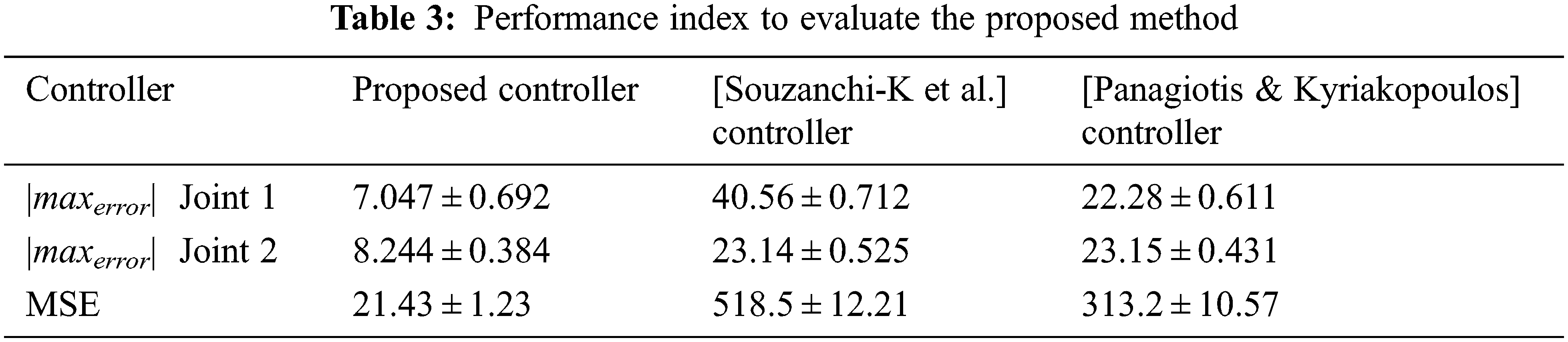
Fig. 4 shows the control system's joint trajectories, and Fig. 5 shows the control efforts under the maximum voltages without chattering. These signals are smooth, which indicates the effectiveness of the proposed controller.

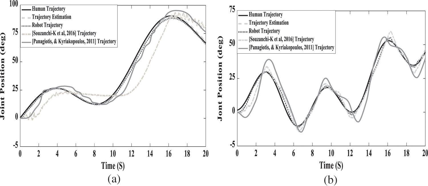
Figure 4: Trajectory performance: (a) for the shoulder joint, (b) for the elbow joint

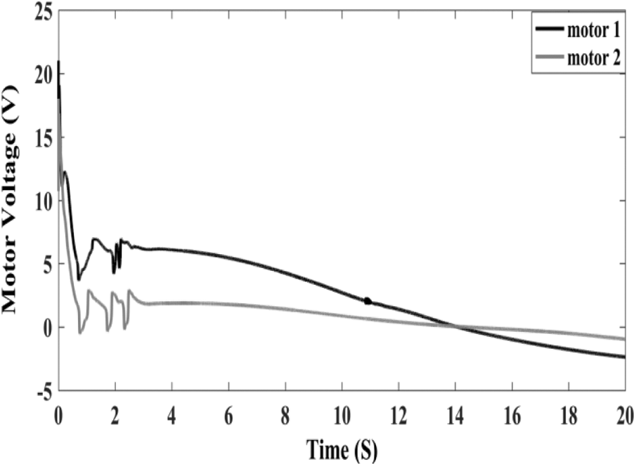
Figure 5: Motors voltage

3  Conclusion

This paper presents a stable adaptive fuzzy strategy to sliding mode control based on the voltage control strategy for an elastic joint robot arm that uses human upper limb EMG signals. The proposed approach is robust against time delay in data transformation channels due to the use of EMG signals and robust against parametric uncertainty and eliminates the system chattering due to an adaptive fuzzy strategy. The Lyapunov analysis proves that the proposed control design guarantees BIBO stability.

For future studies, we hope to study the robustness of the proposed strategy to larger delays in teleoperation application. Also we hope to study isotonic exercises, in addition to the current isokinetic exercise signals. Furthermore, the current experimental work is performed in a 2-D space due to the available measurement hardware. As a next step, we hope to extend our results in 3-D space.

Acknowledgement: The authors would like to express their gratitude to the Sport Science Research Institute of Iran for providing the facilities to implement the experimental tests in this study.

Funding Statement: The authors received no specific funding for this study.

Conflicts of Interest: The authors declare that they have no conflicts of interest or financial ties to disclose.

4  Appendix A.

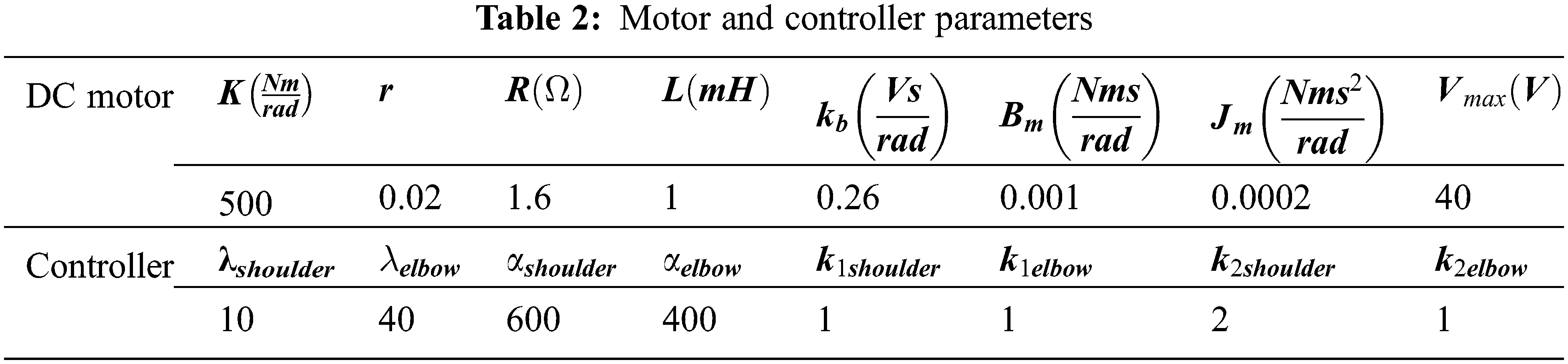
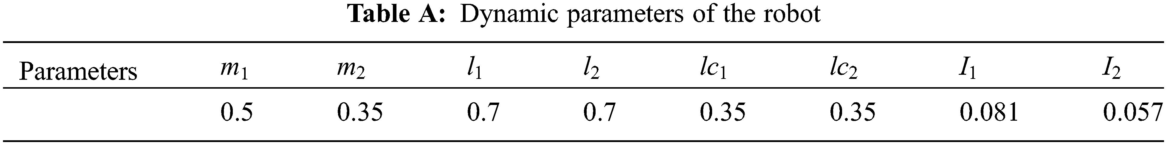
Parameter of robot modeling:

Sq=Sin(q)Cq=Cos(q)

D(q)=[I1+I2+m1lc12+m2(l12+lc22+2l1lc2Cq2)m2(lc22+I1lc2Cq2)+I2m2(lc22+I1lc2Cq2)+I2m2lc22+I2]

C(q,q˙)=[−m2l1lc2Sq2q2.−m2l1lc2Sq2(q1.+q2.)m2l1lc2Sq2q1.0]G(q)=[g(m1lc1+m2l1)Cq1+gm2lc2Cq1+q1m2lc2Cq1+q2]

5  Appendix B.

Experimental setup

This work is licensed under a Creative Commons Attribution 4.0 International License, which permits unrestricted use, distribution, and reproduction in any medium, provided the original work is properly cited.