Intelligent Automation & Soft Computing DOI:10.32604/iasc.2022.022339
Article

False Alarm Reduction in ICU Using Ensemble Classifier Approach

V. Ravindra Krishna Chandar1,* and M. Thangamani2

1Department of CSE, Paavai Engineering College, Namakkal, 637001, Tamilnadu, India
2Department of Information Technology, Kongu Engineering College, Perundurai, 638052, Tamilnadu, India
*Corresponding Author: V. Ravindra Krishna Chandar. Email: ravindrakrishna1234@gmail.com, ravindrakrishna@paavai.edu.in
Received: 04 August 2021; Accepted: 09 December 2021

Abstract: During patient monitoring, false alert in the Intensive Care Unit (ICU) becomes a major problem. In the category of alarms, pseudo alarms are regarded as having no clinical or therapeutic significance, and thus they result in fatigue alarms. Artifacts are misrepresentations of tissue structures produced by imaging techniques. These Artifacts can invalidate the Arterial Blood Pressure (ABP) signal. Therefore, it is very important to develop algorithms that can detect artifacts. However, ABP has algorithmic shortcomings and limitations of design. This study is aimed at developing a real-time enhancement of independent component analysis (EICA) and time-domain detection of QRS that can be used to distinguish between imitation and false alarms. QRS detection is used to examine the waveform values appropriately by calculating the signal values, which are then utilized to identify the areas of high-frequency noise. AHE method is tapped to find the signal saturation values after the removal of such noise values. For artifact detection, Haar Wavelet Transform (HWT) and QRS detection methods are proposed. These operations are performed under the time domain. The classification model is proposed and trained by Fuzzy Neural Network (FNN), Extreme Random Trees (ERTs), and Extreme Learning Machine (ELM).

Keywords: Arterial blood pressure (ABP); haar wavelet transform (HWT); enhanced independent component analysis (EICA); extreme learning machine (ELM); fuzzy neural network (FNN); extreme random trees (ERTs)

1  Introduction

Monitoring patients in the Intensive Care Unit(ICU) is very crucial in today’s medical environment. As a result, there is a clinically significant concern that the patients need additional attention. The resulting noise harms both the patients and the staff. New difficulties about this scary condition have been reported in recent years. For example, according to certain studies, a sleeping issue related to noise in the ICU contributes to deliberate recovery. But, the detrimental impact caused by the increased level of noise in the ICU leads to a false alert, which upsets the medical staff more than the patients [1]. These tiredness alarms do not represent a genuine danger to the sufferers, but they do cause severe harm. This may result in complicated circumstances for hospitals as well as patients. The increasing frequency of alarms and false alarms causes medical experts to become desensitized. There has been numerous research conducted to reduce false alarms in intensive care units in data records. Fallet et al. [2] extracted the HR from- pulsatile waveforms. It uses an adaptive frequency tracking algorithm. The ventricular tachycardia or flutter/fibrillation arrhythmia was identified using the spectral purity in ECGs. Heart rate and spectral purity values-based rules are used to find the alarm veracity. Based on the previous investigation, arterial blood pressure examination was fruitful in reducing the complete false alarms, without restraining any of the true alarm conditions. Arterial Blood Pressure (ABP) was also studied in the recent work.

This work primarily focuses on lowering false alarms through the use of a unique Haar wavelet Wavelet Transform (HWT) and QRS detection in the time domain. In the first stage, signal values are analyzed using Enhanced Independent Component Analysis (EICA) to detect high-frequency noise regions. The AHE approach is used to assess signal saturation values after the noisy samples have been removed. In Haar Wavelet Transform (HWT) and QRS detection, time-domain prediction is utilized to detect artifacts. The proposed categorization model is trained using Fuzzy Neural Networks (FNN), Extreme Random Trees (ERTs), and Extreme Learning Machines (ELM).

The paper is organized as follows, Section 2 deals with the development of false alarm suppression. Section 3 discusses the proposed approach, which includes Enhanced Independent Component Analysis (EICA) for noise removal, signal saturation tactics, HWT and QRS detection for artifact removal, feature extraction, and classification methodology. Section 4 describes the experimental examination of the planned study, and Section 5 is the work's conclusion.

2  Literature Review

Behar et al. [3] assessed ECG quality by using an automated technique. This algorithm is used to identify normal and abnormal rhythms to decrease spurious arrhythmia alarms on ICU monitoring. And it produces highly efficient heart rate prediction. But the decision procedure cannot be utilized in this algorithm for false alarm suppression in ICU.

Aboukhalil et al. [4] examined five categories of false critical ECG arrhythmia alarms by using a multi-parameter ICU database which is produced by the commercial ICU monitoring system. The critical alarm includes ventricular fibrillation/tachycardia, asystole, extreme bradycardia, ventricular tachycardia, and extreme tachycardia. This study does not include non-critical arrhythmia alarms.

Li et al. [5] used Kalman Filter (KF) to estimate the HR and blood pressure. The values of SQI and KF innovation to update the KF sequence. When compared to diastolic ABP calculations, mean ABP calculations were more sensitive to noise. Calculations of diastolic ABP are more reliable than calculations of systolic ABP. Baumgartner et al. [6] proposed an application of data mining to the false alarm rate reduction problem. The work was not focused on obtaining permanent optimal techniques for alarm categorization but temporary outcomes are obtained by using a larger database with evenly distributed alarm kinds. The system evaluated the various classification algorithms like Multi-Layer Perceptron (MLP), Support Vector Machine (SVM), Naive Bayes (NBs), Decision Trees (DT), etc. In ICU monitoring, patient monitoring is significant.

Rani et al. [7] proposed a combination of wavelets such as Daubechies at levels 3 and 4 and Complex Gaussian at scale 1:1:1 and it is executed for QRS complex detection in ECG signal. The baseline drift and denoising reduction are near to zero by the algorithm. The actual QRS peak for 125-patients is 1511 in which 1485 QRS detected and the detection rate is 98.28%. The False-negative values are 0.86% and the False positive value is 3.2%.

Eerikäinen et al. [8] extracted heart beat from signal. F1 -score is used to find the most reliable signal pair by comparing and matching the signals. The best match is selected among the features. Features such as heart rate, signal purity index are extracted from the selected pair, which is used for alarm classification. In addition, selected ECG lead is used for classification. PhysioNet/Computing in Cardiology Challenge 2015 data set is used to evaluate this algorithm.

Amirani et al. [9] decreased false alerts in ICU by using a low complex feature selection technique. Genetic Algorithm (GA) based algorithms are used to assess the shapely estimation of the extracted features. The sensitivity and specificity of the trained replica model are being upgraded by assessing the effect of the collection of different features. The suggested technique has high sensitivity but yields numerical results that are similar to other existing feature selection strategies.

3  Proposed Methodology

Design and Enhanced Independent Component Analysis (EICA) for identifying the noise followed by signal saturation are performed using Haar wavelet transform with QRS detection. Transformation concerning the time domain is performed as the next step. Feature extraction is carried out using automated techniques of ABP followed by QR detection. Finally, classification was performed using diverse classification techniques like Extreme Learning Machine (ELM), Fuzzy Neural Network (FNN), and Extreme Random Trees (ERTs) classifiers for false alarm detection. The integration of multiple classifiers is performed by using Ensemble Classifier Approach (ECA). EC uses heterogeneous classifiers trained on resampling data to increase the variety of their predictions. The proposed methodology shows better enhancement when compared to the existing methods. The proposed model is investigated in detail as given below.

3.1 Data Source Description

The investigation is done using PhysioNet’s MIMIC-II database. It includes 4107 expert-annotated life-threatening arrhythmia alerts, as well as ABP, ECG, and PPG records. The alarms include extreme bradycardia (EB), ventricular tachycardia (VT), asystole (AS), and extreme tachycardia (ET) which is shown in Tab. 1. False alarms are identified by ABP signal measurements. The flow of the proposed technique is shown in Fig. 1

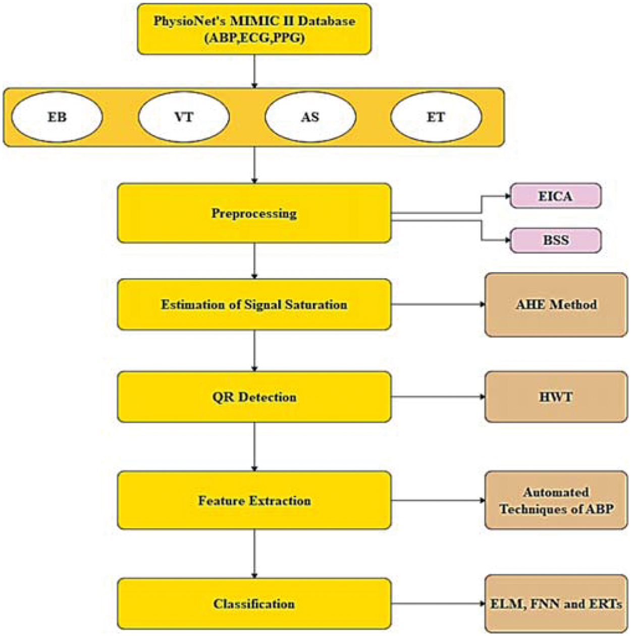
Figure 1: Architecture of proposed model

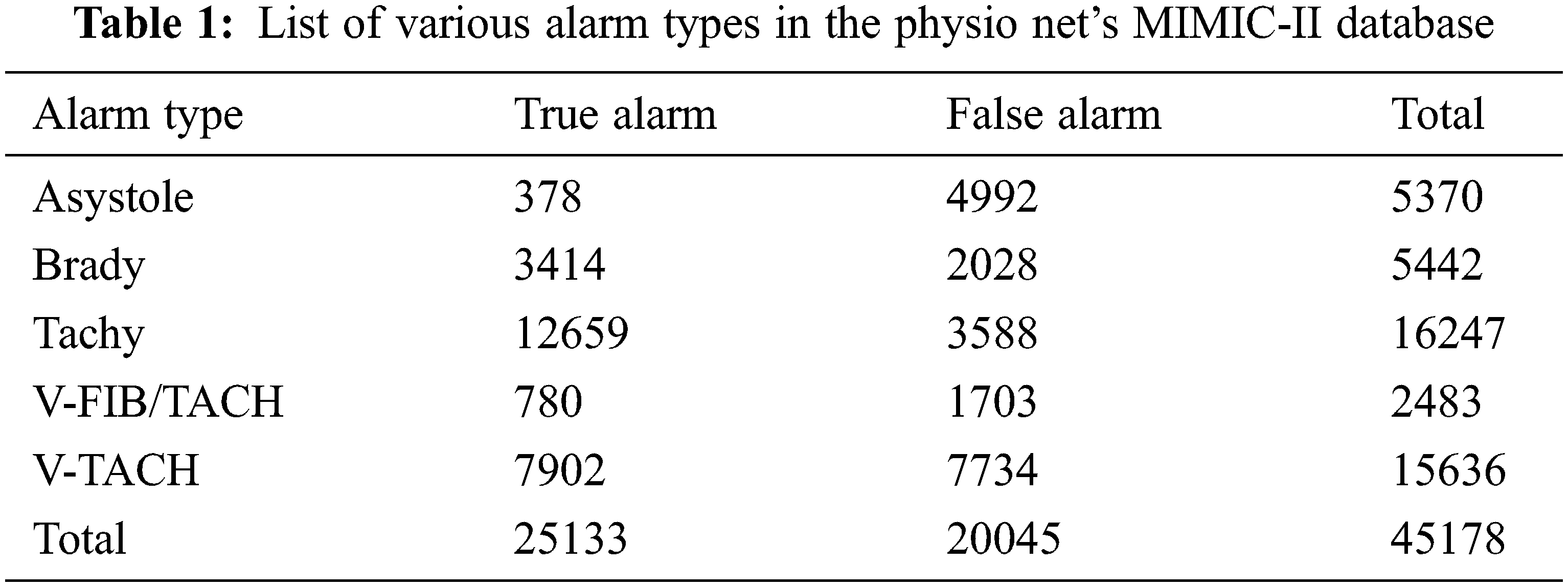
The data for feature selection and feature generation consists of an ABP signal, that is evaluated with 125Hz frequency and heartbeats signal comprising zeros and ones. For every time window, there are two time series for alarm corresponding to 17s and 2125 measurements of length. For every annotated alarm, two arrays are produced. It consists of an appropriate ABP signal during the time interval measurement. There are only 7531 valid ABP signals for entire annotated alarms. In this case, 6 ABP time series are used for each alert, with a total of 45178 samples in the dataset, for evaluation and modeling of the predicted work. Alarms in the dataset are not properly balanced. In each alarm set, there exist more false alarms when compared to true alarms. It leads to the requirement of designing a proper alarm suppression model. This is because machine learning approaches require high accurate datasets. It also requires uniform label distribution.

3.2 Signal Quality for Examining Arterial Blood Pressure (ABP)

The Signal Quality Indices (SQI) are a signal quality and signal noise level computation approach in which there is a fluctuating trust level from the extracted signal waveforms that are acquired from the source data. Algorithm benchmarking SQI is used to reduce the presence of noise and artifacts. An open-source algorithm [10] is used to evaluate the Arterial blood pressure signal quality. If the factors obtained from the blood pressure wave do not fall within the physiological ranges, the signal quality will be bad. When the signal quality is greater than or equal to 0.9, the next beat interval acquired from ABP will not exceed the predefined threshold HR, signaling that the alarm is a false alarm.3.3 Enhanced Independent Component Analysis (EICA)

Blind Source Separation (BSS) corresponds to a mixture of various signals. The observed mixtures are used to extract the sources. Individual signals in series are separated from the mixtures. In this study, Enhanced ICA (EICA) [11] is used to distill the blood pressure signal from the measured ABP signal. It consists of an envelope detection filter, a bandpass filter with 0.04~2 [Hz] bandwidth, a low pass filter with (fc = 0.8 [Hz]) bandwidth, ABP kernel, EICA, and maximum correlation selector for choosing optimal blood pressure signal. High-frequency noises of ABP signal S(k) sampled at k are removed using a 2nd order Butterworth Infinite Impulse Response (IIR) bandpass filter. Then, an envelope detection filter with a mean operator is utilized for feature extraction of blood pressure signals from the ABP signal. The envelope signal is partitioned into a lower envelope signal, rL(k) and upper envelope signal, rU(k) . These are explained from Eqs. (1) to (4).

rmax(k)=max(rBPF(k−m),…rBPF(k−M−1)) (1)

rU(k)=∑q=0Q−1b(q)rmax(k) (2)

rmin(k)=min(rBPF(k−m),…rBPF(k−M−1)) (3)

rL(k)=∑q=0Q−1b(q)rmin(k) (4)

where block size is represented by M. It is used to detect maximum points of filtered ABP signal rBPF(k) . The coefficient of 2nd order LPF is represented by b(k). It has a cutoff frequency of 0.8[Hz] to interpolate rmax(k) and rmin(k) . Average value rM(k) is evaluated by the mean operator by using envelope signals as

rM(k)=rU(k)rL(k) (5)

Eqs. (1)–(4) are used to obtain signals [rL(k) rU(k) rM(k)], which is used to extract ABP signal. The rM(k)=[rL(k)rU(k)rM(k)] is given by,

x(k)=s(k) (6)

where the unknown matrix is represented by A and s(k) represents the original signal vector-like ABP signal and artifacts. An unmixing matrix ‘W’ is used to recover the original signals and it is given by,

s1(k)=Wx(k),A−1≈W (7)

The learning rule is used to update un-mixing matrix W and which is given by,

ΔWα[I−tanh⁡(u)−uT−uuT]XW:super−gaussian[I−tanh⁡(u)−uT−uuT]XW:sub−Gaussian (8)

The ICA estimates the multi-channel output. The optimal respiration signal [12] is extracted by using a maximum correlation selector. The maximum correlation selector compares the reference respiration signal with the ICA output signal to find the channel with the maximum coefficient. EICA output signal is given by,

Cq=∑i=0N−1(Sqi−Sq∗)(Pi−P∗)∑i=0N−1(Sqi−Sq∗)2∑i=0N−1(Pi−P∗)2 (9)

I = Indexmax ([c1, c2….Cq])

where, mean value of EICA output s(k) for q-channel is represented by S*q. P* represents the mean value of the N sample referenced ABP signal. During the absence of artifacts, the reference ABP is measured as the signal. Channel number with maximum correlation value is calculated by using the function Indexmax (.). Fig. 2 portrays the EICA algorithm [13]. From the obtained channel number in Eq. (9), the estimated ABP signal is computed as,

OABP(K)=(k) (10)

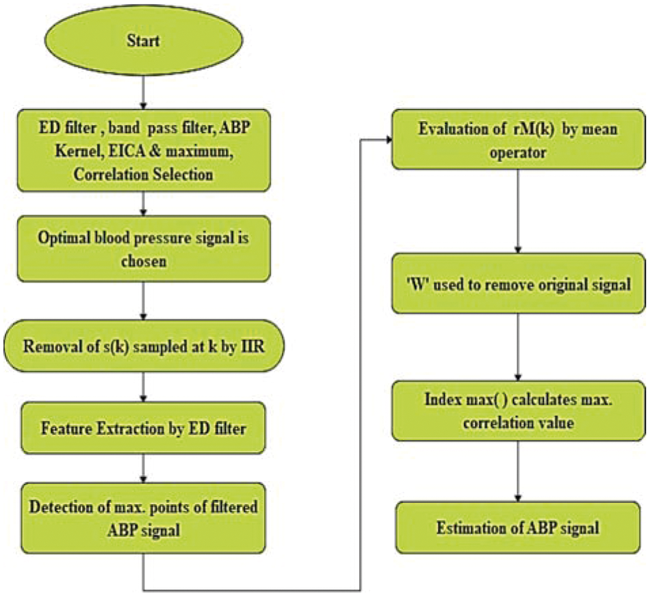
Figure 2: Working procedure of EICA algorithm

3.3 Estimation of Signal Saturation [Maximum & Minimum]

A rapid saturation from a normal ABP to a maximum value ( ABPmax ) displays this type of artifact. Figs. 3a and 3b show the same. In that, maximum value ( ABPmax ) is set to be equal to 200 mmHg ± 10 mmHg. Characteristics ai is estimated by using a hyperbolic tangent function (tanh) and it is given by,

asmax(n,η)=tanhπ.nfs.η).(ABPmax−Adias)+Adias (11)

where saturation rate is given by η(0 < η < 1), Adias represents diastolic ABP, fs gives ABP sampling frequency. Rapid saturation to ABPmax, is obtained with the high value of η.

Figure 3: (a) Artifacts of real signal, (b) ABP signal saturation level to maximum pressure

ABP minimum artifact saturation ( asmin ) is comprised of four types: (1) rapid exponential diastolic saturation, (2) rapid saturation from normal ABP to minimum value ( ABPmin ), (3) exponential increase from ABPmin to ABP value, and (4) gradual transition back to unaffected blood pressure. These four parts are used to produce the artifact boundary. The maximum of ABP defines the upper boundary of the artifact [14]. Square function with independent variable adjusted from 0 to 2.5 defines the lower boundary. The upper boundary is given by,

Asmin(n,η)=[1−tanhπ.nfs.η)] (12)

By decreasing asmin to 90%, the lower part is acquired. The modified upper boundary is given by,

Asmax(n,η)=tanh(π.(n−N2)fs.η) (13)

where the length of boundary is given by n. By reducing asmin by 15%–35% of its original value the lower boundary is obtained. The lower part is the downside of the square function. Figs. 4a and 4b shows the instance of real and artificial asmin artifact respectively.

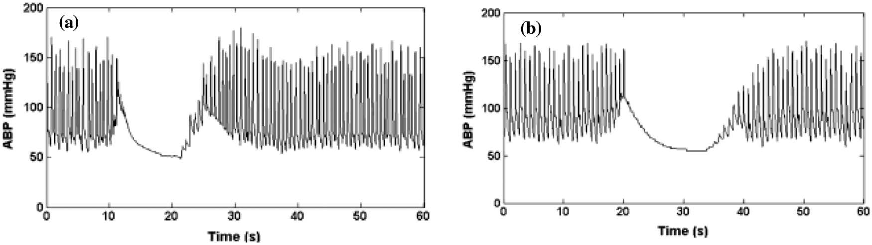
Figure 4: (a) Artifacts of minimum signal value, (b) ABP signal saturation to the lowest pressure

A Brown noise generator is used to simulate the high-frequency artifact. It is implemented by using a bandpass filter. A bandpass filter [15] ranging from 1.5 to 18 Hz is used to filter the noise. Real ABP signals are added with this resultant signal. Figs. 5a and 5b show the instance of real and the artificial Differentiated signal is used to simulate the high-frequency noise. This band-pass filtering is associated with the movement of artifact or disturbance of the transducer.

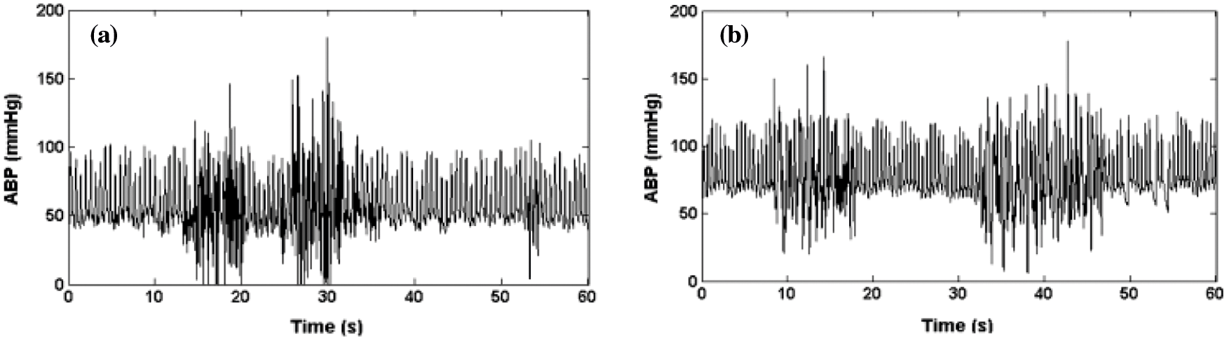
Figure 5: (a) ABP real artifacts of high frequency (b) ABP signal saturation artifacts of high frequency

3.4 Feature Extraction Using Haar Wavelet Transform (HWT) Based QRS

The detection of QRS remains a primary issue in ECG signal analysis. QRS complex comprises three characteristic points and it is signified as Q, R, and S. Some signal details are used to recognize the peaks. The first phase of feature extraction corresponds to R peak recognition. Haar Wavelet Transform (HWT) [16] is used for QRS complex detection.

The energy varies between 3 and 40 Hz in the QRS complex. Sharp edges of signals are related to the zero crossings and modulus maxima of HWT. To analyze time-frequency, HWT is a useful method. In the frequency and time domain, the signals are decomposed into elementary building blocks. These blocks are used to describe the Pattern of regularity in HWT. HWT is a powerful tool for processing signals based on time-domain possibilities.

ABP signals are differentiated from artifacts by using HWT. The information from the ABP signal is hauled out by using wavelets. HWT can be used to examine a signal with fluctuating frequency response. Diverse cutoff frequencies are used to evaluate signals at numerous scales. If it is specified within the data signal, HWT generates a data vector of a similar length. Orthogonal wavelet functions are used to separate the signals. Data points are used to decompose the signals based on wavelet coefficients.

Wavelet scales are discrete in HWT. It breaks down the signal into orthogonal wavelet groups. Applying HWT in discrete time is called discrete-time with continuous HWT. Decimation and continuous filtering processes are being performed to find the optimal level. Signal Length is used to acquire higher levels Redundancy is reduced in this case. The original input signal of DWT is connected with all coefficients from the decomposition end-stage. The reconstruction process is reversed when compared to the decomposition process. Two-pass filters are used to sample and add the coefficients.

C=100.∑I=1nX(I).Y(I)∑I=1nx2(I).∑I=1nY2(I) (14)

where the original ABP signal is given by X; Y represents the reconstructed ABP signal. The Correlation coefficient between all decomposed signals is compared independently with the original ABP signal using the percent of cross-correlation formula as given above to choose the finest coefficient.

3.5 QRS Detector

In all QRS detection algorithm [17], the opening filtering stage is utilized. This is because in QRS complex frequency components fall between 5 and 25 Hz. Additional features in the ABP signal like baseline and noise are suppressed using this filtering. Low pass filter is used to suppress baseline, noise and high pass filters are used to suppress other components.

The bandpass filter is formed by merging the high pass filter and the low pass filter. Its cut-off frequencies range from 5 to 25 Hz for detecting QRS. Threshold values from the filtered signal are used to detect the QRS complex. QRS complex feature possesses a large slope and it is used for detection. Time-varying ABP signal structures cannot be analyzed flexibly by using a QRS detector to noisy signals.

3.6 Classification

Three various classification algorithms have been used to perform classification replicas after feature extraction.

3.6.1 Extreme Learning Machine (ELM)

Extreme Learning Machine (ELM) is based on the neural network. In this work, random initialization of the hidden layer and the input layer weights are used [18,19]. Infinite activation functions of hidden neurons are adjusted by choosing random weights of the hidden and input layer. The pseudo-inverse calculation is used to obtain the output weights [20]. This system will act as a linear system.

Strong generalization performance and fast learning are obtained in this method. The test outcome on different applications and datasets has proven this.

An individual signal sample is assumed as XsεℝF×1 where S represents signal quality index and F represents the number of input features. The classifier output is given as,

yn=∑h=1HWn,hg(∑f=1FWh,fXfs) (15)

where YsεℝF×1 represents the output vector, f and F define the input features and number of input features,h and H define the hidden layer index and the number of hidden neurons respectively. n and N define output layer index and several output neurons, W(1) and W(2) are the weights of the input layer and output layer respectively, g( ) is the activation function of the hidden layer which is a non-linear function. W(1)is randomly fixed and W(2) is computed in single propagation via the output as

yns=∑h=1HWn,hAhs (16)

where,

Ahs=(∑f=1FWh,sXf,s) (17)

The “fan-out” number is signified as hidden layer neurons numbers, H, per input neuron. To acquire superior classification outcomes F must be higher to forecast input and it must be much higher in dimension space. Output neurons are linear and are used to inverse hidden layer outputs. Output targets result in output weights for every classifier. As in matrix equation, W∈ℝN×H gives the matrix with output layer weights wn,h(2) as its elements, and A∈ℝH×S matrix of hidden layer outputs through complete epochs of recording, S. The output matrix Y∈ℝN×S comprises network outputs via entire epochs of recordings as follows in Eq. (18).

Y=WA (18)

Desired outputs of the network are assigned as the target values. Target matrix is distinct as T∈ℝN×S which is the training set outputs through epochs of recordings, as obtained in Eq. (19):

T=WA (19)

The optimization procedure to compute matrix W is determined by computing pseudo-inverse A+∈ℝS×H of A as in Eq. (20).

W=TA+ (20)

where A+=AT(AAT)−1 . The Sum of square errors between network outputs ‘Y’ and target output ‘T’ is reduced in this method by using multiple iterations. ‘Extreme’ corresponds to the network’s maximum learning speed. It has enhanced generalization and lesser training error. This kind of classification is used to obtain false alarm detection in the ABP signal.

3.6.2 Fuzzy Neural Network (FNN)

Followed by this, the second methodology uses a Fuzzy Neural network(FNNs) to approximate complex nonlinear mapping directly to the extracted features from signals. It is a collection of several inputs to give a single output. It is done by forming them sub-rules from the rules with Gj,j=1,2,…,m and Fig. 6 shows the architecture of the FN.

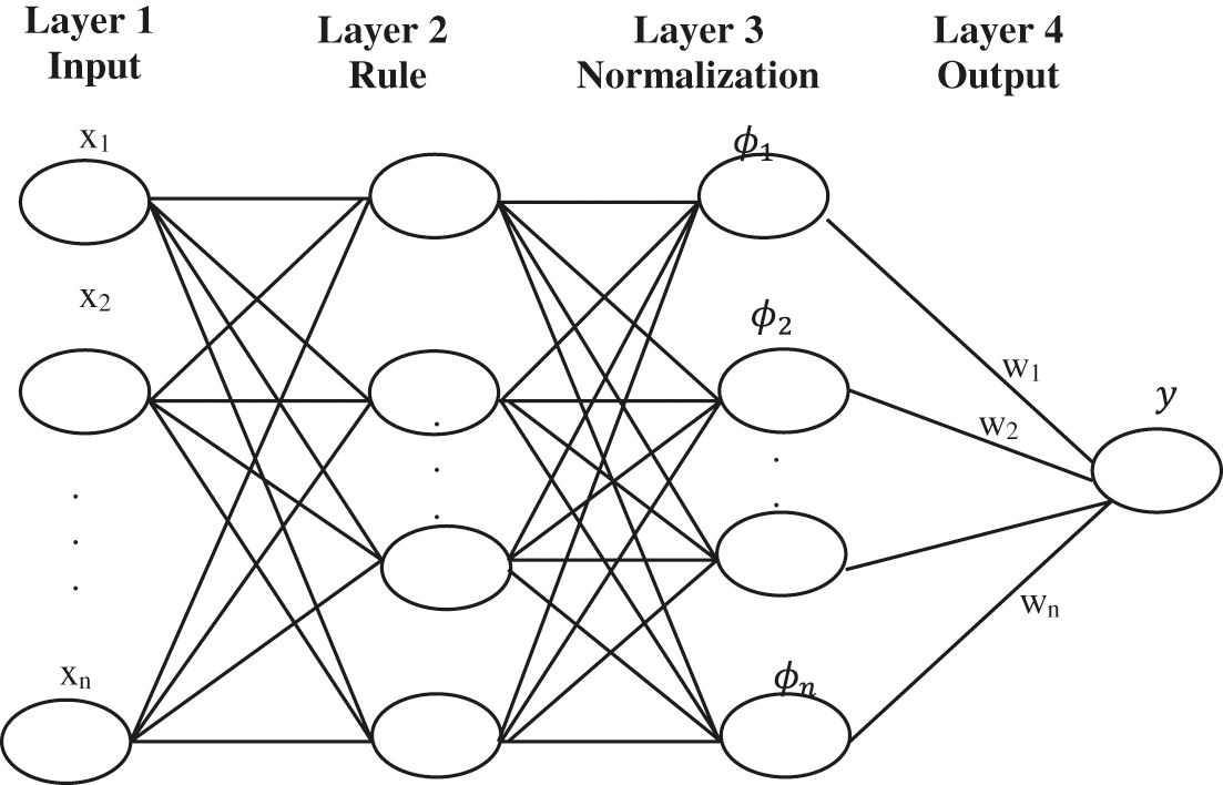
Figure 6: Structure of the FNN system

In the four-layer architecture layer, 1 defines the input and Layer 2 defines the rule. Another two layers formulate the structure of FNNs. Layer three is normalized. Layer four defines the output. The fuzzy rule is given by,

Ifx1is(c1i,σ1i)&x2is(c2i,σ2i)and⋯xnis(cni,σni)thenyisωi (21)

where, center position and width of the fuzzy neurons are given by (c,σ) . The weight of the neuron is given by ω . (c,σ) are regarded as premise parameters. Gaussian functions are used to adopt the membership functions (MFs). T-norm operator is selected as multiplication function. The output variable will equal the weighted summation of the incoming signals, in the center-of-gravity (COG) method of defuzzification and it is given by,

y=∑j=1Lϕjωj (22)

where normalized firing strength of the jth rule is given by ϕj . For classifier, the local rewards are used to measure the local contributions of fuzzy rules and which are given as in,

rlocalj(t)=ϕjr(t),j=1,…L (23)

where fj is the normalized firing strength of the jth rule and r is the system reward.

3.6.3 Extreme Random Trees (ERTs)

Multiple decision trees are generated by Random forests. It is done by sampling the training samples from the datasets. Features are selected randomly from each sample. Here, ‘M’ is the sum of the sample. Sampling is performed randomly but it is consistent while growing the tree. The trees are trained independently. With the benefits of RF, the Extremely Randomized Trees (ERT) algorithm is developed to generate ensemble trees. The training speed is increased because the number of calculations/nodes is reduced. These two methods provide a good outcome for classification purposes. It can increase the training models on huge datasets very lastly. Researchers integrate these methods to biases for N hidden nodes. Random input weights and desired nonlinear activation function has the competency to learn ‘N’ distinct training samples. Unlike traditional methods for modifying network parameters, it carries out a learning algorithm devoid of tuning hidden layer biases and input weights [21]. Traditional approaches for modifying network parameters have significant drawbacks, such as a long training procedure and parameter reliance on multiple layers. Finally, for the evaluation of ensemble performance for each candidate predictor, ensemble predictions are pooled using a weighting factor.

4  Experimental Results

In this investigation, the proposed method and available method's performance are examined by MATLAB. The examined ABP signals are obtained from PhysioBank’s MIMIC databases. In that, signals 23700002 and 05500001 are known as standard clinical data. The ABP signals sampling frequency is 125 [Hz]. The ABP signals 23700002 and 0550001 are cast off for examining the proposed EICA method performance where (cutoff frequency = 0.5 [Hz]) and signals measured in a rest state (devoid of artifacts) and motion state. The experimental output of the EICA experiments is shown in the diagram given below. The signal type in reference with the reference signal shows the smaller difference, but it helps in extracting the original signal outcome. Because the proposed technology suppresses the false alarm signal, the signal distortion was exceptionally low. As a result, the suggested method demonstrates that EICA will deliver a more stable outcome for removing artifacts in the signaltor. To completely estimate the QRS detection algorithm performance, numerous parameters are introduced including false negative (FN), i.e., it fails to generate correct ABP signal, false positive (FP) which signifies false detection of alarm and true positive (TP) i.e., the totality of QRS is correctly detected using the algorithm. By applying all these factors Sensitivity (S), specificity accuracy can be computed. The ABP-related datasets were extracted from PhysioBank’s MIMIC databases for QRS detection using HWT. Each record possesses the following specifications: sampling rate is 360 Hz, signal length is 3600 samples. Fig. 7 given below shows an input of the ABP record. The sensitivity and specificity are computed as:

Sensitivity=PositiveTruealarms(PositiveTruealarms+Negativefalsealarms) (24)

Specificity=Positivefalsealarms(Positivefalsealarms+NegativeTruealarms) (25)

Accuracy=PositiveTruealarms+Positivefalsealarms(PositiveTruealarms+Positivefalsealarms+NegativeTruealarms+Negativefalsealarms) (26)

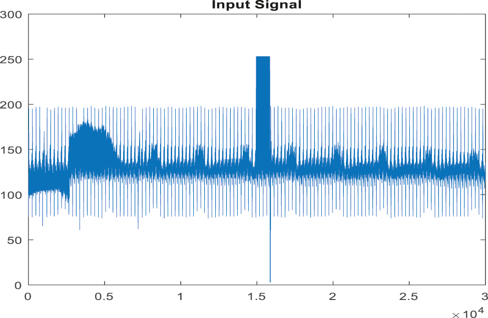
Figure 7: Input signal of ABP record for the false alarm

In the pre-processing phase, filtering the signal is used to extract any artifacts and noise in the ABP signals. In this process, raw ABP signals are used for the processed signal and then filtered for noise removal by EICA as in the given Fig. 8.

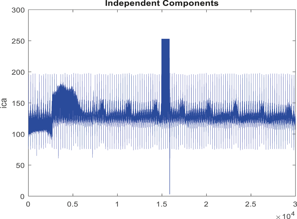
Figure 8: Obtained noise removed signal for false alarm signal

The signals will be rebuilt after the noise interference has been removed. The most important process in the QRS detection procedure is feature extraction and peak tracing. It is utilized to extract the irregularities in the signal [22]. The peak detection method employs HWT in the time domain; the discovered peaks are depicted in Figs. 9, and 10 depicts an ABP record input with a non-false alarm signal.

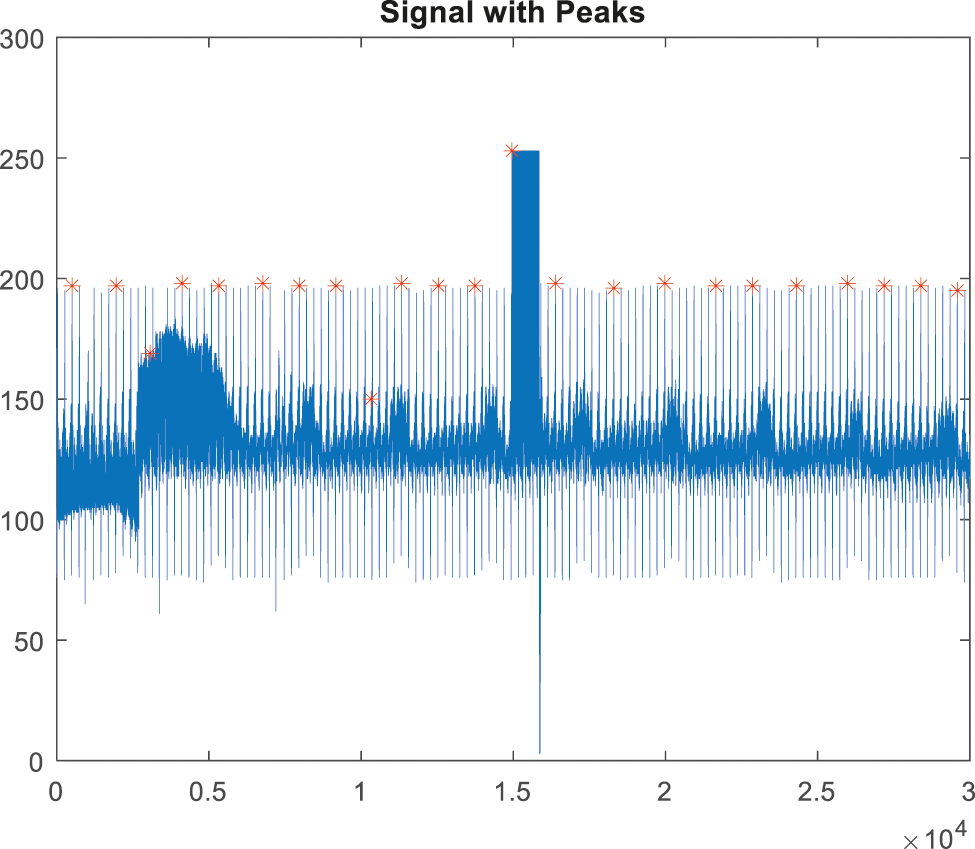
Figure 9: Peak detection for false alarm signal

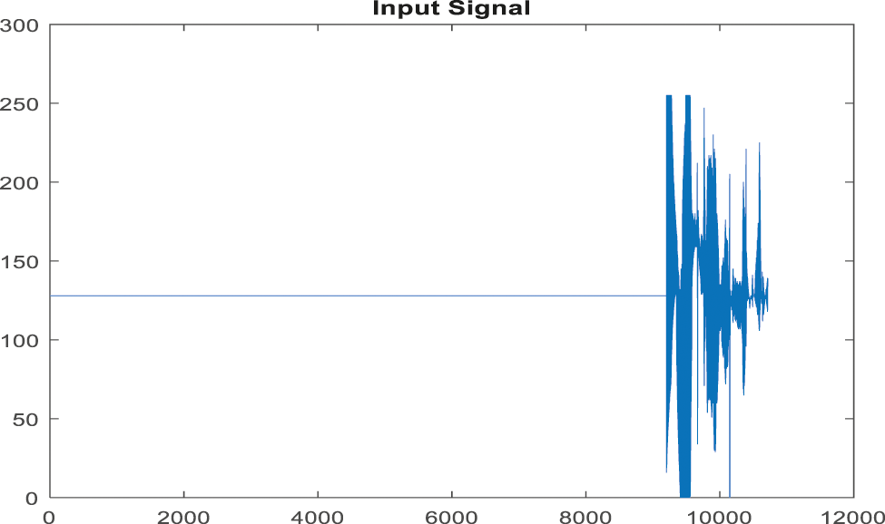
Figure 10: Input signal of ABP record for non-false alarm

Fig. 11 shows a noise removed signal of ABP record with non-false alarm and Fig. 12 shows a peak detection signal of ABP record with non-false alarm, the Tab. 2 explains the comparison results of classifiers.

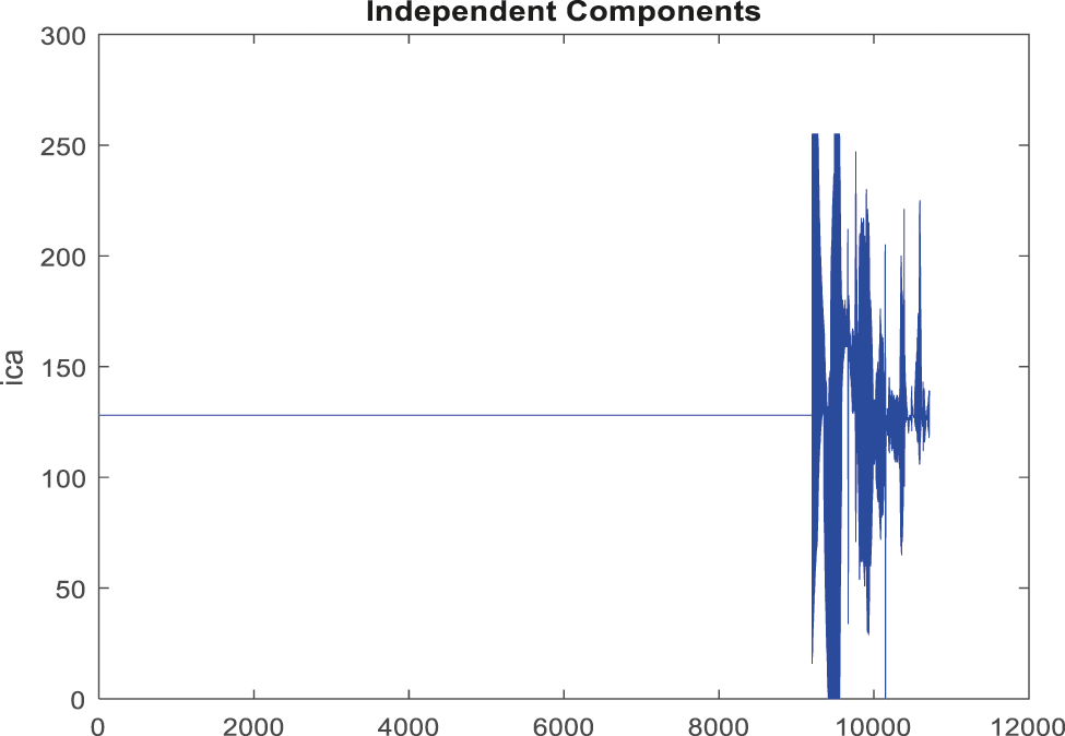
Figure 11: Obtained noise removed signal for non-false alarm

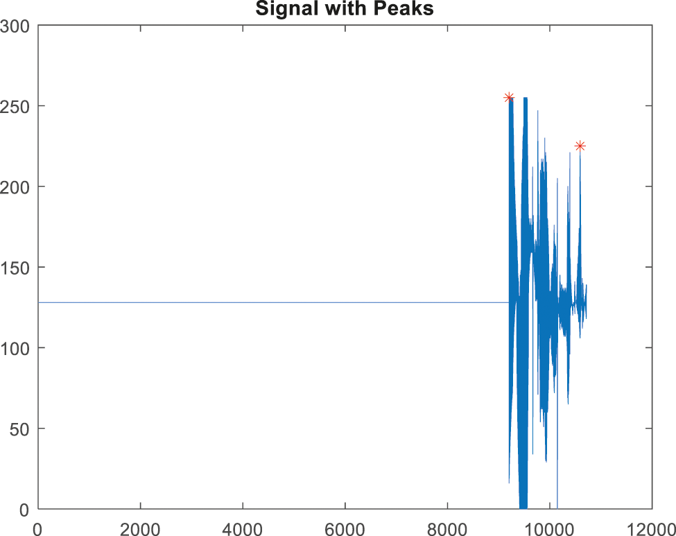
Figure 12: Peak detection for false alarm signal

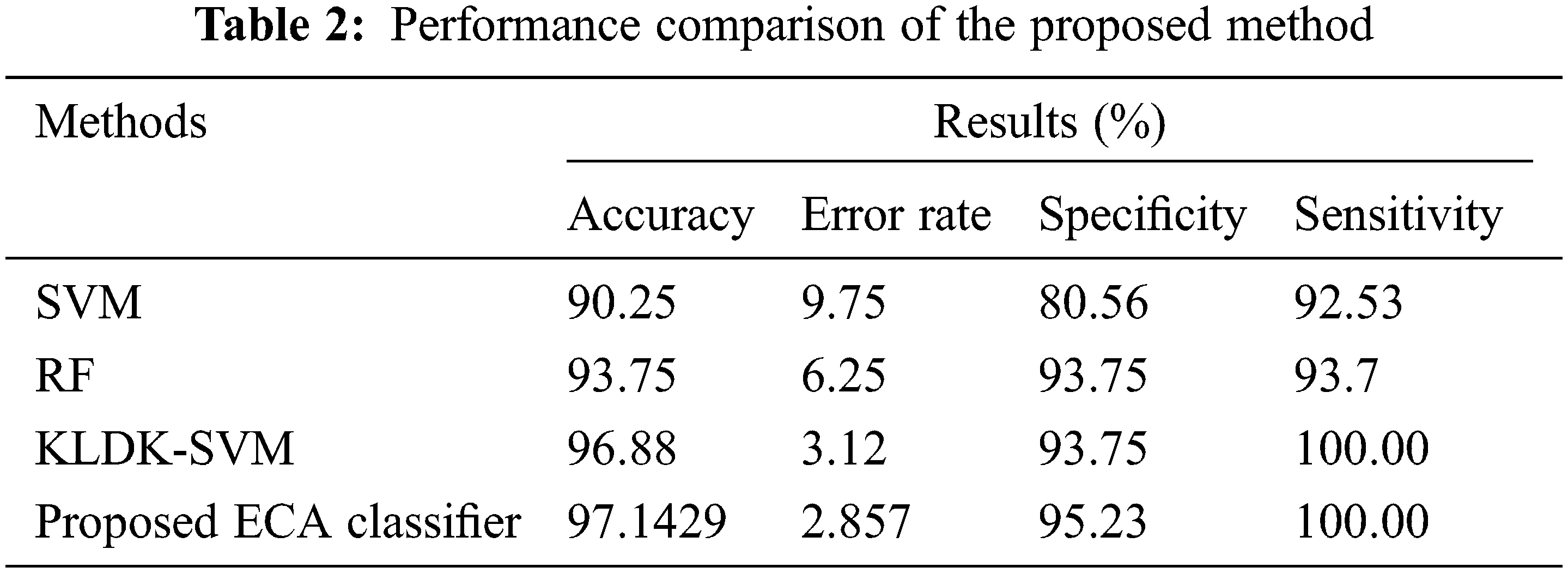
Fig. 13 shows the sensitivity comparison of four classifiers. The proposed ECA classification method provides higher sensitivity results of 100.00%, whereas other classification methods such as SVM, RF, and KLDK-SVM give only 92.53%, 93.7%, and 100.00%.

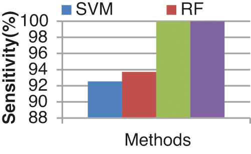
Figure 13: Sensitivity results from the comparison between classifiers

The specificity comparison results of the four different classifiers are shown in Fig. 14. The specificity of the ECA classifier is 95.23%. KLDK-SVM, RF, and SVM provide lesser specificity results of 93.75%, 93.75%, and 80.56% respectively.

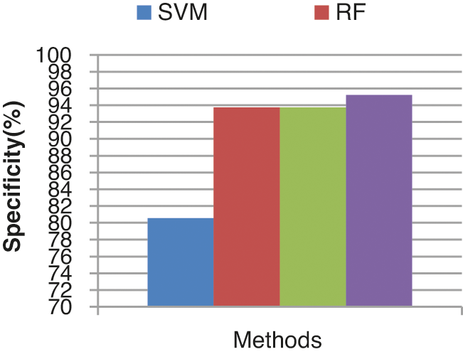
Figure 14: Specificity results comparison vs. classifiers

The overall false alarm detection rate of the various classifiers is shown in Fig. 15. From the results it concludes that the proposed ECA classifier provides an improved false alarm detection rate of 97.129%, the other existing classifiers such as SVM, RF and KLDK-SVM provide lesser false alarm detection rates of 90.25%, 93.75%, and 96.88% respectively.

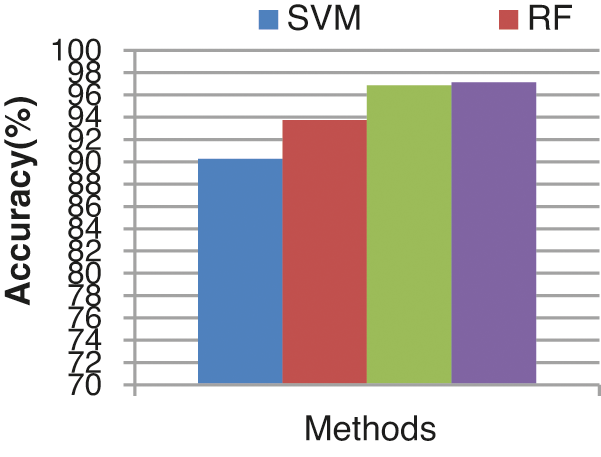
Figure 15: Accuracy results comparison vs. classifiers

Fig. 16 shows the error rate of four different classifiers. The proposed classifier produces a lesser error rate of 2.857%. SVM, RF, KLDK-SVM classifiers produce error rates of 9.75 %, 6.25%, and 3.12% respectively. The error rate of the proposed ECA classifier is less since the proposed work noises are removed by using EICA.

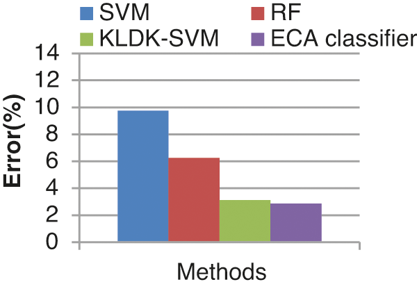
Figure 16: Error rate results from the comparison vs. classifiers

5  Conclusion and Future Work

This study is primarily concerned with the suppression of false alarms with Arterial Blood Pressure (ABP). The key goal of the planned effort is to identify the unique Enhanced Independent Component Analysis (EICA) for recognizing the high-frequency noise region. The signal saturation levels are derived by analyzing the artifacts on a minimal, maximum, or high-frequency artifacts evaluation. In the proposed work, HWT and QRS detection methodologies are used in the temporal domain region. Finally, ensemble predictions are pooled using a weighting factor to evaluate ensemble performance for each candidate predictor. In terms of training the features retrieved from ABP signals and predicting whether the alarm is false or real, the suggested ensemble classification algorithm (ECA) beats prior approaches. Sensitivity, specificity, and accuracy are some of the parameter metrics computed in this work. The proposed classifier has an error rate of 2.857 percent. The error rates for SVM, RF, and KLDK-SVM classifiers are 9.75 percent, 6.25 percent, and 3.12 percent, respectively. Training a large number of features remains a great challenge taken further as a future work where a high-frequency noise ratio is recognized.

Acknowledgement: The authors with a deep sense of gratitude would thank the supervisor for his guidance and constant support rendered during this research.

Funding Statement: The authors received no specific funding for this study.

Conflicts of Interest: The authors declare that they have no conflicts of interest to report regarding the present study.

This work is licensed under a Creative Commons Attribution 4.0 International License, which permits unrestricted use, distribution, and reproduction in any medium, provided the original work is properly cited.