DOI:10.32604/iasc.2022.027349
| Intelligent Automation & Soft Computing DOI:10.32604/iasc.2022.027349 | |
| Article |
Improve Representation for Cross-Language Clone Detection by Pretrain Using Tree Autoencoder
1Nanjing University of Aeronautics and Astronautics, Nanjing, 210008, China
2School of Management Science & Engineering, Nanjing University of Finance and Economics, Nanjing, 210000, China
3Mcgill University, Montreal, H3G 1Y2, Canada
*Corresponding Author: Dafang Li. Email: hdlingnuaa@163.com
Received: 15 January 2022; Accepted: 20 February 2022
Abstract: With the rise of deep learning in recent years, many code clone detection (CCD) methods use deep learning techniques and achieve promising results, so is cross-language CCD. However, deep learning techniques require a dataset to train the models. The dataset is typically small and has a gap between real-world clones due to the difficulty of collecting datasets for cross-language CCD. This creates a data bottleneck problem: data scale and quality issues will cause that model with a better design can still not reach its full potential. To mitigate this, we propose a tree autoencoder (TAE) architecture. It uses unsupervised learning to pretrain with abstract syntax trees (ASTs) of a large-scale dataset, then fine-tunes the trained encoder in the downstream CCD task. Our proposed TAE contains a tree Long Short-Term Memory (LSTM) encoder and a tree LSTM decoder. We design a novel embedding method for AST nodes, including type embedding and value embedding. In the training of TAE, we present an “encode and decode by layers” strategy and a node-level batch size design. For the CCD dataset, we propose a negative sampling method based on probability distribution. The experimental results on two datasets verify the effeteness of our embedding method, as well as that TAE and its pretrain enhance the performance of the CCD model. The node context information is well captured, and the reconstruction accuracy of the node-value reaches 95.45%. TAE pretrain improves the performance of CCD with a 4% increase in F1 score, which alleviates the data bottleneck problem.
Keywords: Code clone detection; autoencoder; abstract syntax tree
In the development of software, to improve efficiency and reduce time cost, some existing codes are often copied-pasted or reused, which produces code cloning. Code cloning refers to two or more identical or similar source code fragments. Code cloning is pretty common, The percentage of which ranges from 5% to 70% [1]. It can improve efficiency and reduce development cost. However, it will increase the maintenance cost, easily to introduce bugs and malicious codes. Therefore, code clone detection (CCD) is needed to find out the cloning pair and mitigate the negative effects of code cloning.
Many CCD methods have been proposed, including traditional methods [2–4] and machine learning based methods [5–7]. They primarily handle single language CCD. However, developers often need to develop the same functionality in different programming languages for different software systems [8–11] (e.g., C/C# for Windows phones, Java for Android phones, and Objective-C for iPhone [12]) to achieve compatibility and adoptability [13,14]. These bring the cross-language clones. Most of the existing studies only consider a single language, the research on CCD is limited to a single language. Single language CCD methods cannot detect clones between different languages. Thus, Cross-language CCD methods need to be developed. Some cross-language CCD have been proposed, including traditional methods [12,15,16] and machine learning based methods [17–19]. Machine learning based methods achieve better results but require a labeled dataset for model training [20]. Due to the difficulty of dataset collecting, the dataset is typically small or has a gap between real-world cloning. This leads to a data bottleneck problem: data scale and quality issues will cause that model with a better design can still not reach its full potential. For example, the work of [17] created a CCD dataset by fetching source code from competitive programming websites. The dataset is small and very different from the source code in a real-world system.
To mitigate this, we consider using unsupervised learning to pretrain the model on a large-scale dataset, then use the trained model to fine-tune in the small dataset. We use an autoencoder framework. The pretrain is done by doing an auto-encode-and-decode task on ASTs. It does not require any label and the dataset can be fetched from the internet as much as we want. By training an autoencoder through unsupervised learning in a large-scale dataset, a better result can be achieved in the downstream CCD task with the pretrain encoder, especially when the amount of labeled data is small. We make the following contributions:
1) We design a novel embedding method for AST nodes, including type embedding and value embedding. We design a tree-based distance and a tree-based Glove algorithm for type embedding, use a Gated Recurrent Unit (GRU) [21] plus LSTM [22] autoencoder for value embedding.
2) We propose a novel architecture that uses an autoencoder to pretrain on a large-scale dataset then fine-tunes the encoder in CCD. This will reduce the dataset requirement. We design a tree structure encoder and decoder, which combine as a tree autoencoder (TAE).
3) We present three training techniques for TAE, including “encode and decode by layers”, the use of node-level batch size and a tree splitting strategy. We propose a probability distribution based negative sampling method for the training on the CCD dataset.
4) We verify our proposed methods in a self-collecting dataset and an open-source cross-language CCD dataset. Experimental results verify the effeteness of the node embedding method, as well as that TAE and its pretrain enhance the performance of the CCD model.
In the next section, we will list some related works, then we will present our method in Section 3. In Section 4, we will present the experimental setup and results. Finally, we conclude our work in Section 5.
In this section, we will present some related works about CCD and some other approaches for vector embedding representation.
Recently, the rise of neural networks has led to better development of CCD. Many researchers have designed neural network models for CCD and achieved promising results. AST-based neural network (ASTNN) [5] is a neural network designed for code AST to extract features from ASTs and perform CCD. It first does a word embedding pretrain on ASTs, then trains a neural network using the pretrain embedding. However, its pretrain performs on node sequences obtained by depth-first search (DFS) on ASTs, which loses tree structure information and cannot obtain a good embedding.
Clone detection with learning to hash (CDLH) [6] uses a tree-based LSTM for CCD. The tree-based LSTM encodes the AST into a vector and then uses a hash layer to map the vector into a hamming space (hash code) [23]. Finally, the CCD prediction is determined by the hash codes. Similarly [7] also uses a tree-based LSTM to extract features from ASTs. The features of the two ASTs are input into a classifier or a similarity measurement model. Then, a loss function is designed to train the whole model. Both [6] and [7] must transfer the ASTs into binary trees. However, if transform ASTs into binary trees, extra nodes are added, and the tree size and depth can dramatically increase. This will affect the encoding of the tree, weaken the model’s ability to capture more realistic and complex semantics, and affect the performance.
For cross-language CCD, C2D2 [15] is the first cross-language CCD tool. It detects clones between C# and Visual Basic .NET languages using Code Document Object Model (CodeDOM) as an intermediate representation. However, the requirement of an intermediate representation makes it limited. Cheng et al. [16] proposed CLCMiner that uses the code revision histories for CCD without an intermediate language. However, the revision histories it relies on may not be available in the real application. So, it has limitations.
Perez et al. [17] proposed a novel AST node embedding method: a tree-based skip-gram. After the node embedding, the AST is flattened into a sequence by DFS and then fed into the LSTM. Finally, a classifier is used to predict the clone pair. However, the window size in the paper cannot be increased to capture further node context information. When increasing the window size, the method not only fails to obtain a better representation but also introduces more noise, resulting in information flattening problem (related types’ embedded vectors in space distribution are more dispersed and lower polymerized).
CroLSim [18] uses the application programming interface (API) documentation to find relationships among the API calls used by different languages. It presents a deep learning based vector learning method to identify semantic relationships. However, this method depends on the quality of the API documentation.
2.2 Vector Representation Approaches
Vector representation refers to projecting objects (e.g., words, nodes, tokens) in high-dimensional space into a continuous vector space with a much lower dimension. It maps the object into a fixed dimension vector [24]. Since the source code and natural language are similar in some ways, vector representation techniques like word embedding used in natural language processing can also apply to source code related work such as CCD.
There are word embedding methods, including Word2vec [25] and Glove [26]. Word2Vec is a successful method used in large-scale word representation. It obtains word-pair information for model training by sliding a fixed-length window on the sentences in the corpus. Two models are proposed in Word2Vec: continuous bag-of-words model (CBOW) and skip-gram model. The former uses the context to predict the central word, while the latter uses the central word to predict the context. Glove improves Word2vec by using corpus’s global statistics, making it quite efficient. However, these methods are designed only for sequence data, and cannot apply to tree structure data such as AST.
Besides the word embedding, there are other vector representation techniques, some of which are designed for source code. Peng et al. [27] designed a “coding criterion” method to build vector representations of AST nodes, making it possible to use deep learning for program analysis. Yu et al. [28] proposed a new token embedding method, position-aware character embedding (PACE). It splits a token into characters, then the token’s embedding is the weighted sum of one-hot encoding of all characters [29]. This embedding technique requires no training and can apply to arbitrary tokens. However, this method that weighting by position is asymmetric in position: the weight of the front position is bigger than the weight of the back position.
The work of [30] uses a random walk method on AST, which combines DFS and breadth-first search (BFS) simultaneously to obtain a sequence to train the skip-gram model. After obtaining the embedding of AST nodes, sentence embedding, a lightweight approach, is used to obtain the representation of the entire tree. Finally, it detects code clones by similarity measure using Euclidean distance. However, it uses all the ASTs in the dataset to generate the sequence, leading to the wrong context information when sliding the window (nodes on two different ASTs appear in the window at the same time).
The overview of our method is illustrated in Fig. 1. There are two major parts: TAE pretrain and CCD. For TAE pretrain, we first fetch source codes from the database, then get the AST data and do filtration to obtain the Base AST data. Then, the Base AST data is extracted and filtered to build three datasets: Type Embedding Dataset, Value Embedding Dataset, and Pretrain AST Data. We train the models and get the trained encoder of TAE, which will be used in the CCD model. For CCD, we preprocess the CCD dataset and create Pair Data. After training the CCD model, we can use it for evaluation or use it as a CCD tool.

Figure 1: Method overview
Our method uses the AST of the source code. We first have to preprocess the source code: extract the AST, and do a transformation (i.e., refer to the AST syntax of the target language and simplify the AST). Inspired from the node representation format in [7], which uses a type-content pair to represent an AST node, we use the format type-value pair to represent an AST node. The preprocessing of the source code is not our focus. To do computation on the AST, we use fixed dimension vectors to represent nodes (i.e., embedding). Our node embedding includes type embedding and value embedding.
Our type embedding method is based on Glove [26], a word embedding method that uses corpus’s global statistics (co-occurrence matrix). Its target is to optimize the following function:
where V is vocabulary size, wi and wj are the left and right embedding of the i-th word, X is the co-occurrence matrix. f is a weighting function. The window of Glove can only be used in sequential data, not tree structure data. To improve Glove to adapt the tree structure data, we first propose a novel tree-based distance d(x, y). For two different nodes a and b in the same tree:
1)
2) If a and b are inheritance relationship (a is an ancestor/descendant of b), then
3) If a and b are not inheritance relationship, find the “closest” (the deepest) common ancestor c, then
The tree-based distance visually can be interpreted as that every two children of the same node are connected by a shortcut. It’s easy to prove that the proposed distance satisfies the three conditions of a legal distance definition (non-negativity, symmetry, and satisfying the triangle inequality).
We define a node’s sequentiality based on whether its children’s order matter: if a node’s children matter in order and the number of children is not fixed, we call it a sequential node (or it’s sequentiality), otherwise we call it a non-sequential node (or it’s non-sequentiality). We add five auxiliary losses according to five additional tasks. One is to predict a type’s sequentiality, other four are to predict special relationship: parent-child relationship, grandpa-grandchild relationship, near-sibling relationship (sibling nodes whose indexes differ by 1), near-near-sibling relationship (sibling nodes whose indexes differ by 2). Their losses denote as Ls, La, Lb, Lc, Ld, requiring vector S and matrix A, B, C, D. The loss of Glove denotes as Lg. The final loss is as follows:
Si is the statistics about type ti, can be positive or negative (depend on sequentiality). Aij is the statistics about ti and tj (ti is on the left of tj, “left” and “right” is based on the node order by DFS on the AST, the front is left, the behind is right), can be positive or negative (depend on the relationship between ti and tj). B, C and D are similar to A. We have (Lb, Lc and Ld are similar to La):
where λ is an exponent hyperparameter to soften the weight coefficient, BCE is the binary cross entropy. The co-occurrence matrix X can be represented as a linear combination of specific distance co-occurrence matrices:
The whole step of tree-based Glove is the following: “slice” the window on the ASTs to get all matrices and optimize Eq. (2) by sampling index pairs from V to get the embedding matrix
In the value embedding phase, we use a GRU + LSTM autoencoder framework. GRU encodes value into a fixed-length vector, and then LSTM decodes the vector to reconstruct the original value. In the encoding phase, two special tokens are added before and after the word to get the input sequence, including the start of the word and the end of the word, denoted as and . Then, feed the sequence into the encoder to get the output vector. In the decoding phase, distribute the output vector in time step and feed them into the LSTM, then apply the linear layer to the outputs to get the predicted sequence. The illustration can be seen in Fig. 2. We add two additional auxiliary losses according to two additional tasks:
1) Word classification: predict whether the word/value is an identifier, a real number or the others.
2) Character classification: predict each character’s class. We categorize 128 ASCII characters, and into 7 classes: , , digits, capital letters, lowercase letters, non-printing characters (control characters, ASCII range is in 0 ∼ 31) and other characters.

Figure 2: Autoencoder of value embedding
Finally, the whole loss is the following:
where en+1 is , yw and zi are the classification labels, and CE is the cross entropy.
Our TAE model includes an encoder and a decoder, both use a tree LSTM. LSTM [22] is proposed for handling sequence data and cannot handle tree structure data like AST. To deal with tree structure data, [31] proposed Child-Sum Tree-LSTMs:
where σ is the sigmoid function,
where xs is the input (node embedding, concatenating of type embedding and value embedding) of node s.

Figure 3: TAE's tree LSTM and decoder
The decoder of TAE contains a node embedding decoder (type classifier + value decoder) and a Tree LSTM Decoder (inner decoder + outer decoder + end of children (EOC) classifier):
where y is the input of the decoder LSTM, not the node embedding of s. The inner decoder decodes hs into
where T is the nodes set of an AST tree, |T| is the node count, and ns is the children count of node s. Since the tree root is not a child to any node, hroot is not used in Eq. (37). The number of hidden states we need to compute Lchildren is |T| − 1, we have

Figure 4: TAE's encoding and decoding
The encoding/decoding of each node depends on the encoding/decoding of its children/parent. The encoding/decoding has to be from down/top to top/down. With this, we introduce an “encode and decode by layers” strategy: group nodes by layers and encode/decode multiple nodes simultaneously in a layered fashion [33]. For the encoding/decoding of multiple trees, we first sort the trees by depth. Then group the nodes by layers and encode/decode them layer by layer. Such a strategy takes full advantage of parallel computing capability. When training on the AST data, we don’t train on a batch of ASTs. Instead, we train on a batch of nodes. The node count of every step depends on the AST (i.e., the size of the batch is dynamic). We use a hyperparameter “max node count” to imply the max node count in a training step. If several ASTs’ total node count is smaller than the batch size, we group them in a batch. If an AST’s node count is bigger than the batch size and smaller than the max node count, we use a tree splitting strategy that split it into several subtrees to make every subtree’s node count smaller than the batch size. Then, train on these subtrees one by one while preserving every subtree’s root encoding to provide for the parent subtree.
Our CCD model uses a siamese-based architecture neural network [34], including an AST extractor, two encoders and a classifier. The AST extractor extracts AST from the source code. The encoder uses TAE’s encoder that encodes the whole AST into a fixed-length vector. The CCD classifier accepts two vectors and does a binary classification to predict if the two code fragments are clone pair. The training code pairs are obtained from the dataset by sampling similar to [17], except for the sampling of negative samples.
To create code pairs, first, sample a code fragment (anchor) and then sample a positive sample and n negative samples. The positive sample is randomly selected from the set of code clones of the current anchor fragment. For negative samples, we create a candidate set and randomly select m samples from it to run into the model. Finally, select n samples whose predicted scores are top-n highest as negative samples. We use a probability distribution method. We denote the selected positive fragment as a, denote code fragment dataset of the target language as C, and g(a) is the AST node count of a. Then we use
as a probability measure of a. Finally, the candidate set of a is created with a hyperparameter
Such a candidate set makes sure its size is always 2ε|C|.
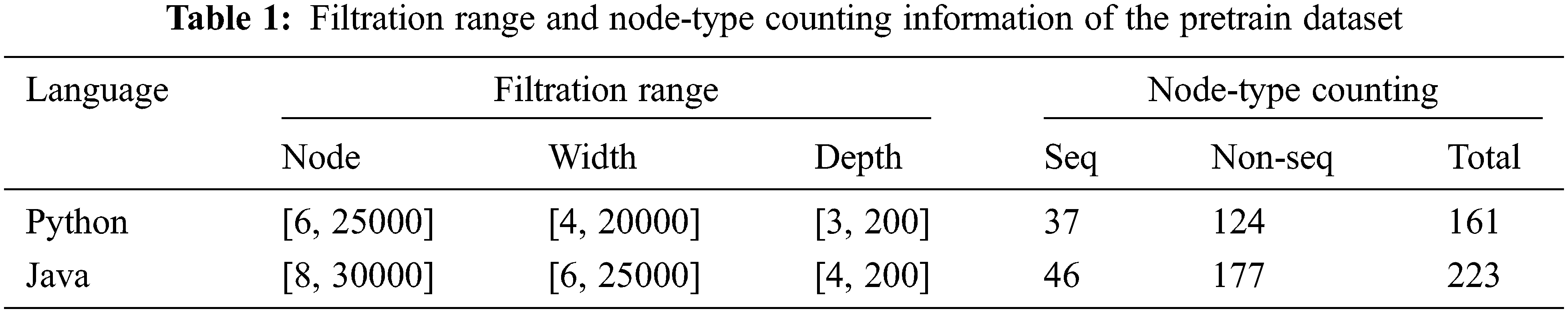
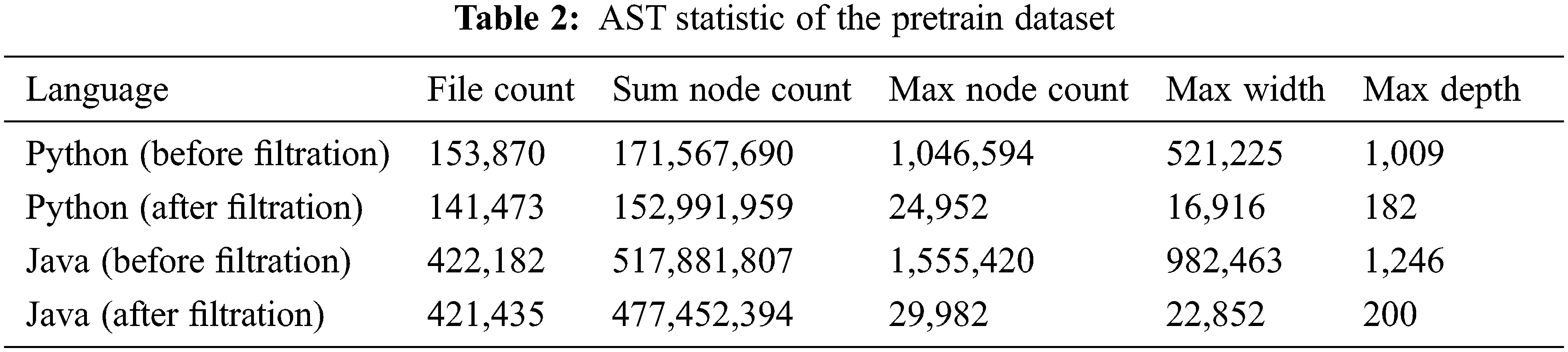
In our experiments, we use two datasets: a pretrain dataset for node embedding and TAE pretrain and a CCD dataset for cross-language CCD [17]. The pretrain dataset is created by fetching repositories whose starts are not less than 1k from GitHub. The raw data is about 100G (python + java). We extract ASTs and do filtration to get the base AST data. Filtration range and node-type counting information are listed in Tab. 1 (“seq” is short for sequential), AST statistic is listed in Tab. 2. The CCD dataset mainly contains folders of source codes, including 20828 java files (46 lines/file on average) and 23792 python files (13 lines/file on average). There are 576 folders, each folder represents a problem. Files in the same folder have the same functionality, thus two files or code fragments from the same folder can be seen as a clone pair.
We conduct experiments on a six-core window-10 machine of 16 GB memory with a Nvidia GeForce GTX 1650 GPU of 4 GB memory. Pytorch (https://pytorch.org) is used to build and train our model. Python built-in ast module (https://docs.python.org/3.9/library/ast.html) and javalang (https://github.com/c2nes/javalang) are used to extract python/java raw AST. We use Adam [35] as the optimization algorithm, except for type embedding, we use stochastic gradient descent (SGD). The learning rate is 0.01 if not specified. For brevity, in node embedding and TAE pretrain, we only show python results.
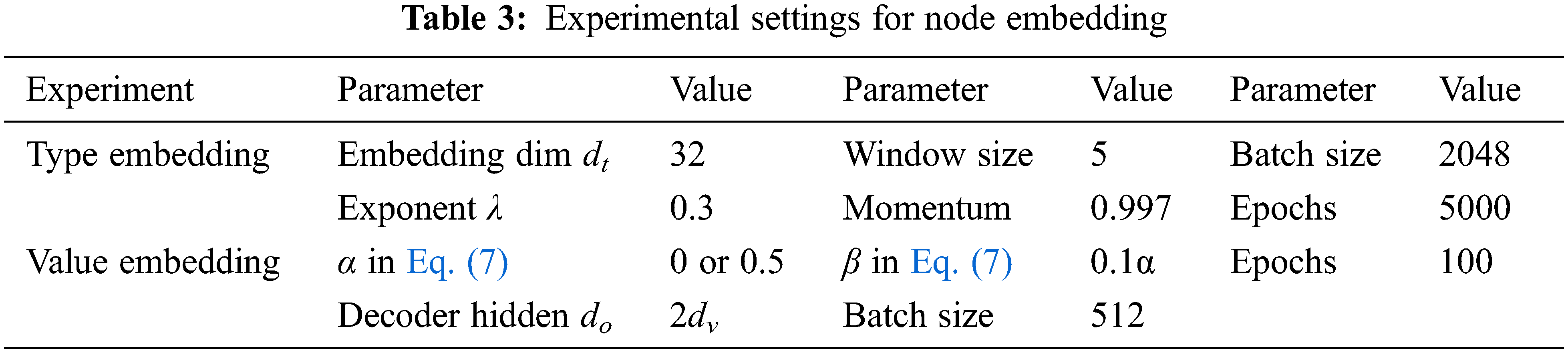
Node embedding includes type embedding and value embedding. The experimental settings are in Tab. 3. For type embedding, the f in Eq. (1) is similar to the Glove paper, the ratio in Eq. (2) is [0.9497, 0.01, 0.015, 0.01, 0.0003, 0.015]. The experimental result is visualized in Fig. 5 using T-SNE [36–38]. The red dots are sequential node-types and the blue dots are non-sequential node-types. The figure shows that the related node-types gather nicely, the context information and semantics are well preserved. If not using normalization, the points in the figure will be more dispersed [39–41]. With the proposed tree distance and the normalization, there is no need to worry about the information flattening problem. The window size can increase to 7 even more, unlike [17] that can only use a window size of 2 and does not include siblings.

Figure 5: T-SNE visualization of python AST type embedding
For the value autoencoder training, we first filter some words whose length is bigger than a predefined threshold (here we use 100). And words with length no more than this threshold will be used as the base dataset. Then, the base dataset is split into a training set and a testing set at a ratio of 9:1. The fine-tuning learning rate of the char embedding layer is 0.0001. Four criteria are used to evaluate the models:
■ char_acc: characters level accuracy.
■ s_char_acc: characters level accuracy in strict mode.
■ word_acc: word-level accuracy.
■ len_acc: word length match accuracy, the ratio of whose are predicted in the correct length.
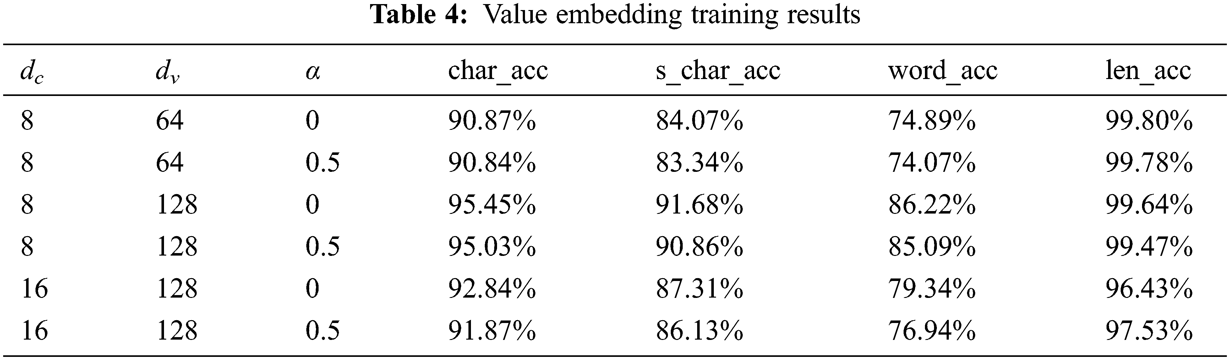
The experimental result is in Tab. 4. The configuration with

Figure 6: Python value embedding reconstruction accuracy
In the training of TAE, the whole AST, which comes from the data preprocessing, will be involved. In the training phase, we process the source code on the fly via multi-processing. We filter the base AST data by max node count, the left AST data is also split into a training set and a testing set at a ratio of 9:1. To speed up the value embedding phase, we pre-compute the top 10000 most frequent value to build a lookup table. We use the scheduled sampling [32] for the input of TAE’s outer decoder. The probability p decays in each epoch/step via cosine decay (can be epoch-level or step-level):
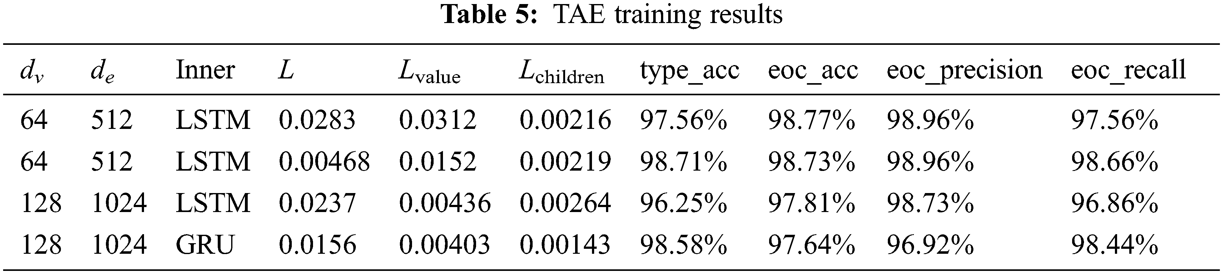
The ratio we used in Eq. (33) is [0.2, 0.1, 0.2, 0.5]. We set the max node count to 500, set the batch size to 300, and set epochs to 10. The type embedding model fine-tuning learning rate is 0.00002. The type classifier, value decoder, and EOC classifier all adopt 2 layers of feed-forward neural network. The experimental result can be seen in Tab. 5. As can be seen in the table, the second configuration achieves the best result in criteria. We use the encoder of this configuration as the encoder of our CCD model.
We first do a cross-language code clone classification experiment. The CCD dataset is randomly split into a training set and a testing set at a ratio of 9:1. For negative sampling, we use n = 10, m = 4, ɛ = 0.1. We set the max node count to 1024, set the batch size to 2 × 512, and set epochs to 20. If the encoder comes from pretrain, then we set its fine-tuning learning rate to 0.0001. The experimental result of classification is depicted in Tab. 6. From the result, we can see that our proposed tree LSTM based CCD model outperforms the sequence LSTM based CCD model. And the TAE pretrain enhances the performance of the CCD model. Next, we use the trained model to do the CCD experiment. We randomly select 500 code fragments from the test set and run the model for all pairs to determine clone pairs. The clone detection result is depicted in Tab. 7. As can be seen in the table, our proposed CCD model outperforms the sequence LSTM based CCD model as well, and CCD benefits from the pretrain. The work of [17] uses sequential LSTM to encode the sequence. It obtains token sequence from AST by DFS, doing so will lose the AST tree structure information. Unlike [17], our Tree LSTM does the encoding directly on the AST, which preserves the AST structure information. So, our method still obtains a better result without pretrain.


Our TAE training is based on file level, a more fine-grained level (e.g., class/function level) can be considered in future work. With the trained TAE, code fragments can be represented as a vector, different languages correspond to different vector spaces. We can consider using an unsupervised learning framework like CycleGAN [39], to do one more pretrain on different languages’ encoding spaces, which will build a connection between different languages without the help of any label. This may benefit CCD, which can be a key future work. In addition, our value embedding is a little bit overhead, and our CCD model’s loss is simple. A better value embedding method and a better CCD loss are needed in future work.
In this work, we focus on cross-language CCD using an autoencoder to pretrain on a large-scale dataset. We first introduce the node embedding method, including type embedding and value embedding. Then, we give detail about our TAE model, including the encoder and the decoder. We also present techniques about the training of TAE, including the “encode and decode by layers” strategy and the batch size design. Next, we talk about the CCD model and our negative sampling strategy. In the end, we evaluate our method in a self-collecting dataset and an open-source cross-language CCD dataset. The experimental results verify the effeteness of our node embedding method, as well as that TAE and its pretrain enhance the performance of the CCD model. The node context information is well captured and the reconstruction accuracy of the node-value reaches 95.45%. TAE pretrain improves the performance of CCD with a 4% increase in F1 score, which alleviates the data bottleneck problem.
Funding Statement: This work was supported by the National Key R&D Program of China (Grant No. 2021YFB3100700), the National Natural Science Foundation of China (Grant No. 62032025, 62076125, U20B2049, U20B2050, 61702236), the Natural Science Foundation of Jiangsu Province (Grant No.BK20200418, BE2020106), the Guangdong Basic and Applied Basic Research Foundation (2021A1515012650), the Shenzhen Science and Technology Program (JCYJ20210324134810028), the Natural Science Foundation of Jiangsu Province (Grant No.BK20200418, BE2020106).
Conflicts of Interest: The authors declare that they have no conflicts of interest to report regarding the present study.
1. S. Ducasse, M. Rieger and S. Demeyer, “A language independent approach for detecting duplicated code,” in 1999 Int. Conf. on Software Maintenance, Oxford, England, UK, pp. 109–118, 1999. [Google Scholar]
2. T. Kamiya, S. Kusumoto and K. Inoue, “Ccfinder: A multilinguistic token-based code clone detection system for large scale source code,” IEEE Transactions on Software Engineering, vol. 28, no. 7, pp. 654–670, 2002. [Google Scholar]
3. L. Jiang, G. Misherghi, Z. Su and S. Glondu, “Deckard: Scalable and accurate tree-based detection of code clones,” in 29th Int. Conf. on Software Engineering, Minneapolis, MN, USA, pp. 96–105, 2007. [Google Scholar]
4. H. Sajnani, V. Saini, J. Svajlenko, C. K. Roy and C. V. Lopes, “Sourcerercc: Scaling code clone detection to big-code,” in Proc. of the 38th Int. Conf. on Software Engineering, Austin, TX, USA, pp. 1157–1168, 2016. [Google Scholar]
5. J. Zhang, X. Wang, H. Zhang, H. Sun, K. Wang et al., “A novel neural source code representation based on abstract syntax tree,” in Proc. of the 41st Int. Conf. on Software Engineering, Montreal, QC, Canada, pp. 783–794, 2019. [Google Scholar]
6. H. Wei and M. Li, “Supervised deep features for software functional clone detection by exploiting lexical and syntactical information in source code,” in 26th Int. Joint Conf. on Artificial Intelligence, Melbourne, Australia, pp. 3034–3040, 2017. [Google Scholar]
7. L. Büch and A. Andrzejak, “Learning-based recursive aggregation of abstract syntax trees for code clone detection,” in 26th IEEE Int. Conf. on Software Analysis, Evolution and Reengineering (SANER), Hangzhou, China, pp. 95–104, 2019. [Google Scholar]
8. C. Ge, Z. Liu, J. Xia and L. Fang, “Revocable identity-based broadcast proxy re-encryption for data sharing in clouds,” IEEE Transactions on Dependable and Secure Computing, vol. 18, no. 3, pp. 1214–1226, 2021. [Google Scholar]
9. C. Ge, W. Susilo, J. Baek, Z. Liu, J. Xia et al., “Revocable attribute-based encryption with data integrity in clouds,” IEEE Transactions on Dependable and Secure Computing, vol. 21, no. 5, pp. 1–12, 2021. [Google Scholar]
10. Y. J. Ren, Y. Leng, Y. P. Cheng and J. Wang, “Secure data storage based on blockchain and coding in edge computing,” Mathematical Biosciences and Engineering, vol. 16, no. 4, pp. 1874–1892, 2019. [Google Scholar]
11. C. Ge, W. Susilo, Z. Liu, J. Xia, P. Szalachowski et al., “Secure keyword search and data sharing mechanism for cloud computing,” IEEE Transactions on Dependable and Secure Computing, vol. 18, no. 6, pp. 2787–2800, 2021. [Google Scholar]
12. X. Cheng, Z. Peng, L. Jiang, H. Zhong, H. Yu et al., “Mining revision histories to detect cross-language clones without intermediates,” in Proc. of the 31st IEEE/ACM Int. Conf. on Automated Software Engineering, Singapore, pp. 696–701, 2016. [Google Scholar]
13. C. Ge, W. Susilo, J. Baek, Z. Liu, J. Xia et al., “A verifiable and fair attribute-based proxy re-encryption scheme for data sharing in clouds,” IEEE Transactions on Dependable and Secure Computing, vol. 21, no. 7, pp. 1–12, 2021. [Google Scholar]
14. L. Fang, M. Li, Z. Liu, C. Lin, S. Ji et al., “A secure and authenticated mobile payment protocol against off-site attack strategy,” IEEE Transactions on Dependable and Secure Computing, vol. 21, no. 9, pp. 1–12, 2021. [Google Scholar]
15. N. A. Kraft, B. W. Bonds and R. K. Smith, “Cross-language clone detection,” in Proc. of the Twentieth Int. Conf. on Software Engineering & Knowledge Engineering (SEKE’2008), San Francisco, CA, USA, pp. 54–59, 2008. [Google Scholar]
16. X. Cheng, Z. Peng, L. Jiang, H. Zhong, H. Yu et al., “Clcminer: Detecting cross-language clones without intermediates,” IEICE Transactions on Information and Systems, vol. 100, no. 2, pp. 273–284, 2017. [Google Scholar]
17. D. Perez and S. Chiba, “Cross-language clone detection by learning over abstract syntax trees,” in Proc. of the 16th Int. Conf. on Mining Software Repositories (MSR), Montreal, Canada, pp. 518–528, 2019. [Google Scholar]
18. K. W. Nafi, B. Roy, C. K. Roy and K. A. Schneider, “Crolsim: Cross language software similarity detector using api documentation,” in 18th IEEE Int. Working Conf. on Source Code Analysis and Manipulation (SCAM), Madrid, Spain, pp. 139–148, 2018. [Google Scholar]
19. K. W. Nafi, T. S. Kar, B. Roy, C. K. Roy and K. A. Schneider, “Clcdsa: Cross language code clone detection using syntactical features and api documentation,” in 34th IEEE/ACM Int. Conf. on Automated Software Engineering (ASE), San Diego, CA, USA, pp. 1026–1037, 2019. [Google Scholar]
20. Y. J. Ren, J. Qi, Y. P. Cheng, J. Wang and O. Alfarraj, “Digital continuity guarantee approach of electronic record based on data quality theory,” Computers, Materials & Continua, vol. 63, no. 3, pp. 1471–1483, 2020. [Google Scholar]
21. K. Cho, B. V. Merriënboer, C. Gulcehre, D. Bahdanau, F. Bougares et al., “Learning phrase representations using rnn encoder-decoder for statistical machine translation,” in Proc. of the 2014 Conf. on Empirical Methods in Natural Language Processing, Doha, Qatar, pp. 1724–1734, 2014. [Google Scholar]
22. S. Hochreiter and J. Schmidhuber, “Long short-term memory,” Neural Computation, vol. 9, no. 8, pp. 1735–1780, 1997. [Google Scholar]
23. Y. J. Ren, F. J. Zhu, S. P. Kumar, T. Wang, J. Wang et al., “Data query mechanism based on hash computing power of blockchain in internet of things,” Sensors, vol. 20, no. 1, pp. 1–22, 2020. [Google Scholar]
24. Y. J. Ren, J. Qi, Y. P. Liu, J. Wang and G. Kim, “Integrity verification mechanism of sensor data based on bilinear map accumulator,” ACM Transactions on Internet Technology, vol. 21, no. 1, pp. 1–20, 2021. [Google Scholar]
25. T. Mikolov, I. Sutskever, K. Chen, G. S. Corrado and J. Dean, “Distributed representations of words and phrases and their compositionality,” in Advances in Neural Information Processing Systems 26: 27th Annual Conf. on Neural Information Processing Systems, Lake Tahoe, Nevada, United States, pp. 3111–3119, 2013. [Google Scholar]
26. J. Pennington, R. Socher and C. D. Manning, “Glove: Global vectors for word representation,” in Proc. of the 2014 Conf. on Empirical Methods in Natural Language Processing, Doha, Qatar, pp. 1532–1543, 2014. [Google Scholar]
27. H. Peng, L. Mou, G. Li, Y. Liu, L. Zhang et al., “Building program vector representations for deep learning,” in 8th Int. Conf. on Knowledge Science, Engineering and Management, Chongqing, China, pp. 547–553, 2015. [Google Scholar]
28. H. Yu, W. Lam, L. Chen, G. Li, T. Xie et al., “Neural detection of semantic code clones via tree-based convolution,” in Proc. of the 27th Int. Conf. on Program Comprehension, Montreal, QC, Canada, pp. 70–80, 2019. [Google Scholar]
29. Y. J. Ren, K. Zhu, Y. Q. Gao, J. Y. Xia, S. Zhou et al., “Long-term preservation of electronic record based on digital continuity in smart cities,” Computers, Materials & Continua, vol. 66, no. 3, pp. 3271–3287, 2021. [Google Scholar]
30. Y. Gao, Z. Wang, S. Liu, L. Yang, W. Sang et al., “TECCD: A tree embedding approach for code clone detection,” in 2019 IEEE Int. Conf. on Software Maintenance and Evolution, Cleveland, OH, USA, pp. 145–156, 2019. [Google Scholar]
31. K. S. Tai, R. Socher and C. D. Manning, “Improved semantic representations from tree-structured long short-term memory networks,” in Proc. of the 53rd Annual Meeting of the Association for Computational Linguistics and the 7th Int. Joint Conf. on Natural Language Processing of the Asian Federation of Natural Language Processing, Beijing, China, pp. 1556–1566, 2015. [Google Scholar]
32. S. Bengio, O. Vinyals, N. Jaitly and N. Shazeer, “Scheduled sampling for sequence prediction with recurrent neural networks,” in Advances in Neural Information Processing Systems 28: Annual Conf. on Neural Information Processing Systems, Montreal, Quebec, Canada, pp. 1171–1179, 2015. [Google Scholar]
33. Y. J. Ren, Y. Leng, J. Qi, K. S. Pradip, J. Wang et al., “Multiple cloud storage mechanism based on blockchain in smart homes,” Future Generation Computer Systems, vol. 115, pp. 304–313, 2021. [Google Scholar]
34. J. Bromley, J. W. Bentz, L. Bottou, I. Guyon, Y. Lecun et al., “Signature verification using a “siamese” time delay neural network,” International Journal of Pattern Recognition and Artificial Intelligence, vol. 7, no. 04, pp. 669–688, 1993. [Google Scholar]
35. D. P. Kingma and J. Ba, “Adam: A method for stochastic optimization,” in 3rd Int. Conf. on Learning Representations, San Diego, CA, USA, 2015. [Online]. Available: http://arxiv.org/abs/1412.6980. [Google Scholar]
36. L. Maaten and G. Hinton, “Visualizing data using t-sne,” Journal of Machine Learning Research, vol. 9, no. 11, pp. 2579–2605, 2008. [Google Scholar]
37. T. Li, N. P. Li, Q. Qian, W. Xu, Y. Ren et al., “Inversion of temperature and humidity profile of microwave radiometer based on bp network,” Intelligent Automation & Soft Computing, vol. 29, no. 3, pp. 741–755, 2021. [Google Scholar]
38. X. R. Zhang, W. F. Zhang, W. Sun, X. M. Sun and S. K. Jha, “A robust 3-D medical watermarking based on wavelet transform for data protection,” Computer Systems Science & Engineering, vol. 41, no. 3, pp. 1043–1056, 2022. [Google Scholar]
39. J. Y. Zhu, T. Park, P. Isola and A. A. Efros, “Unpaired image-to-image translation using cycle-consistent adversarial networks,” in Proc. of the IEEE Int. Conf. on Computer Vision, Venice, Italy, pp. 2223–2232, 2017. [Google Scholar]
40. Y. J. Ren, F. Zhu, J. Wang, P. Sharma and U. Ghosh, “Novel vote scheme for decision-making feedback based on blockchain in internet of vehicles,” IEEE Transactions on Intelligent Transportation Systems, vol. 23, no. 2, pp. 1639–1648, 2022. [Google Scholar]
41. X. R. Zhang, X. Sun, W. Sun, T. Xu and P. P. Wang, “Deformation expression of soft tissue based on BP neural network,” Intelligent Automation & Soft Computing, vol. 32, no. 2, pp. 1041–1053, 2022. [Google Scholar]
 | This work is licensed under a Creative Commons Attribution 4.0 International License, which permits unrestricted use, distribution, and reproduction in any medium, provided the original work is properly cited. |