DOI:10.32604/iasc.2022.023962
| Intelligent Automation & Soft Computing DOI:10.32604/iasc.2022.023962 | |
| Article |
Air Pollution Prediction Using Dual Graph Convolution LSTM Technique
1Department of Electronics and Communication Engineering, Anna University, University College of Engineering Dindigul, Dindigul, 624622, India
2Department of Applied Cybernetics, Faculty of Science, University of Hradec Králové, 50003, Hradec Králové, Czech Republic
3Department of Computer Science, College of Computers and Information Technology, Taif University, P. O. Box 11099, Taif, 21944, Saudi Arabia
4Department of Mathematics, Faculty of Science, Mansoura University, Mansoura, 35516, Egypt
5Department of Computational Mathematics, Science, and Engineering (CMSE), Michigan State University, East Lansing, MI, 48824, USA
*Corresponding Author: Mohamed Abouhawwash. Email: abouhaww@msu.edu
Received: 28 September 2021; Accepted: 21 December 2021
Abstract: In current scenario, Wireless Sensor Networks (WSNs) has been applied on variety of applications such as targets tracking, natural resources investigation, monitoring on unapproachable place and so on. Through the sensor nodes, the information for the applications is gathered and transferred. The physical coordination of these sensor nodes is determined, and it is called as localization. The WSN localization methods are studied widely for recent research with the study of small proportion of the sensor node called anchor nodes and their positions are determined through the GPS devices. Sometimes sensor nodes can be a IoT device in the network. With despite this, among the various applications, air pollution and air quality monitoring having many issues on how to place the sensor network in a wide area to monitor the air pollutants level such as carbon dioxide (CO2), nitrogen dioxides (NO2), particulate matter (PM), sulphur dioxide (SO2), ammonia (NH3) and other toxic gases involved in human and industrial activities. The responsibility of the WSN in air quality monitoring is to be positioning the sensor nodes in the large area with low cost and also gather the real time data and produce the monitoring system as an accurate one. In this proposed work, deep learning-based approach called dual graph convolution and LSTM (Long Short-Term Memory) network based (air quality index) AQI predictions were performed. This uses the infrared based technology to measure the CO2, temperature and humidity, Geo statistic method and low power wireless networking. Accuracy of the proposed system is maximum of 95% which is higher than existing techniques.
Keywords: WSN; deep learning; air quality monitoring; graph convolutional neural network; LSTM; air pollution
As day from industrial revolution till today, new innovation and technological demands makes more industries across the world. Though it meets demands of technological crisis, it does pollute the society. An industry makes the fast urbanization of the society. The effluents, contaminated particles from industries mix with outside of air and damages the quality. Quality of air degradation leads to pollution which is biggest threat to public wellbeing. It’s essential to scrutinize the quality of air in hour by hour to alert the society. Wireless sensor network with IoT is used in our research to estimate air quality using artificial intelligence techniques.
Main causes of air pollutants are nitrogen dioxide, carbon monoxide, ozone and sulphur dioxide gases [1]. Sometime air quality is affected by particulate matter present in it. There are two types, PM 2.5 and PM 10, which is main pollutants and causes some health hazard. PM 2.5 is a air particle in the atmosphere with diameter less than the 2.5 fm and 10 fm. These particles can easily enter to nasals and causes severe respiratory problems as well as cardiac related problems [2]. Nowadays pollution control board uses air quality monitoring sensors in main cities in the country to check the quality through online in minute by minute. This station monitors the quality and mention the severity of pollution level in different areas in maps. It is very challenging to monitor the quality and classify the pollutant in real time. Conventional techniques still need to enhance with developed artificial intelligence technology. In our research we use deep learning model for high accuracy prediction. The main contribution in this article is,
1. Deep learning model is designed to improve the prediction of air pollutant level.
2. Sensor data is processed using Graph convolutional neural network by learning the pollutant and its characteristics.
3. Graph LSTM is used to process the decision of the graph convolutional neural network.
Rest of article is presented with 5 chapters. Second chapter deals with literature survey of the air monitoring and processing techniques. Third chapter deals with implementation of proposed model and its architectural design. Chapter four evaluates the experimental results and shows the comparison of traditional methods. Chapter five evaluates the work and concludes the research with future scope.
In [2] proposed an outdoor pollution weather prediction and monitoring system. It consists of sensing unit for the pollution such as sensors MQO7 for carbon monoxide (CO), sensor SDS021, sensor B43F for NO2 and aeroqual ozone (O3). These sensing techniques are used to gather the air pollutant level such as PM2.5, PM10, CO, NO2 and O3. They collected data from dec 2019 to feb 2020. They evaluate their experiment for AQI predictions with the approaches such as linear regression and artificial neural network model (ANN). They also compared their experiment with existing machine learning models like linear, ridge, Lsso, Bayes, Lars, Hubers, Lasso Iars, elastic Net regressing and Stochastic gradient descent (SGD). They obtain the efficient result on linear regression compared to other algorithms.
In [3] proposed an AI model to measure the air pollutant. This model was trained with the various air quality indexes with fuzzy logic and meta-heuristics methods such as particle swarm optimization (PSO) and simulated annealing (SA). This model measures the concentration of air pollutants such as NO2, CO and weather variables like humidity, relative humidity, temperature, and absolute humidity. The model is evaluated with the statistical measures such as mean absolute error and correlation coefficient. Among the models, PSO performs better to predict the air pollutants.
In [4] proposed a wireless system to monitor the health issues. Wireless system can be used to monitor the concentration of temperature, humidity, and CO2. The air quality is predicted using the auto regressive integrated moving average method. For feedback control, fuzzy theory has been used as an energy saving mechanism. This model obtains the improved accuracy from 3.19% to 3.47% and error rate was less than 7.5%. With the help of fuzzy model, this proposed model saves 55% energy of the system.
In [5] proposed an infrared based sensor indoor air quality monitoring system. This sensor measures the concentration of air pollutant such as humidity, CO2 and temperature, geo statistics and minimum power networking. This model use (market based economic dispatch) MBED LPC 1768 board for data transfer used ZigBee module. This model can also use to predict the spatial data. In [6] proposed a air quality monitoring based wireless sensor network in Doha. These wireless sensor units are communicated to the server for transferring the real time. The data are stored at server for intelligent processing. They used the tools such as system of R software and open-air package for analysis.
In [7] proposed a review about the graph neural network and its applications. They can also be discussed about the problems and future research. Jiang et al. [8] proposed about the using social network/media for air quality monitoring. For air prediction issue, the petroleum gas university analyzed the methods such as genetic algorithms, artificial neural network, decision tress, k nearest neighbor, logistic regression [9]. In [10] examined and analyze the AQI system. They predicted the result as PM2.5 pollutant maintain the air quality better for safety living.
In [11] proposed a wireless sensing network for air pollutant real time update using (generic ultraviolet sensors technologies and observations) GUSTO. This proposed one lack in Internet of things in wireless sensing. In [12] proposed a model to monitor air pollution and developed a mobile based applications with cloud framework. This is not tested for outdoor sites. In [13] reviewed about the air pollution monitoring system based on stationary and dynamic air pollution monitoring system with classification. These monitoring systems are compared in terms of microcontroller used, analyzed pollutant from sensors, communication devices used and performance. They can also be discussed about the advantages and disadvantages of air pollution monitoring system.
In [14] build cost efficient energy model for air pollution monitoring system with wireless network. They used hierarchical based genetic algorithm for this monitoring. This can address the sensor node issue with minimum energy. This Hypercube Based Generic Algorithm (HBGA) will reduce the energy consumption of the network. This model can monitor the spatial and temporal data of air quality.
In [15] reviewed about the indoor air pollution monitoring using wireless network. They can stats the relationship among indoor air pollution and their corresponding risks. They discussed the methods for the purpose of cyber physical system. They also discussed about the microcontrollers used for this monitoring and their respective challenges with the future research directions.
In [16] stated about internet of things (IoT) with cloud on various applications like smart home, e-health care, industrial IoT, smart transport. IoT with cloud enhance the WSN model for smart environmental data transmission with authentication. The system efficiency is improved by utility pattern of IoT and cloud with edge nodes. It is considered as a confidence assessment system by balancing the incoming load dynamically with cloud and edge. Result of this work creates optimal secured IoT infrastructure for WSN in future.
In [17] proposed a load balancing problem, utilization issues and energy optimization in cloud computing. They use Server distinction weights which are active correspondingly for balancing load in the network. It minimizes the cloud makespan in environment. In [18] proposes speech enhancement technique for quality in network using generative adversarial network. It enhances the signal of speech in network. In [19] implements proficient design method for signal processing and reconfiguration. It helps to manage field programmable gate array in to reconfigure network for high performance. In [20] proposes content based retrieval of video using histogram of oriented gradient (HOG) for high accurate video selection. Image is given as input and histograms of image helps to retrieve the video.
In this proposed work, dual graph convolutional network has been used to process the data captured from the sensor nodes. The gathered data are then learned with the AQI characteristics using graph LSTM (G-LSTM). The proposed system overview is shown in Fig. 1. The architecture consists of the components for data gathering, data analysis and networking, monitoring using proposed method and sending data feedback about the air quality. Recently, IoT devices help to collect the air quality information using its sensors and transmit to centralized data server. A sensor sends and receives air quality data in distributed network using parallel computing framework.
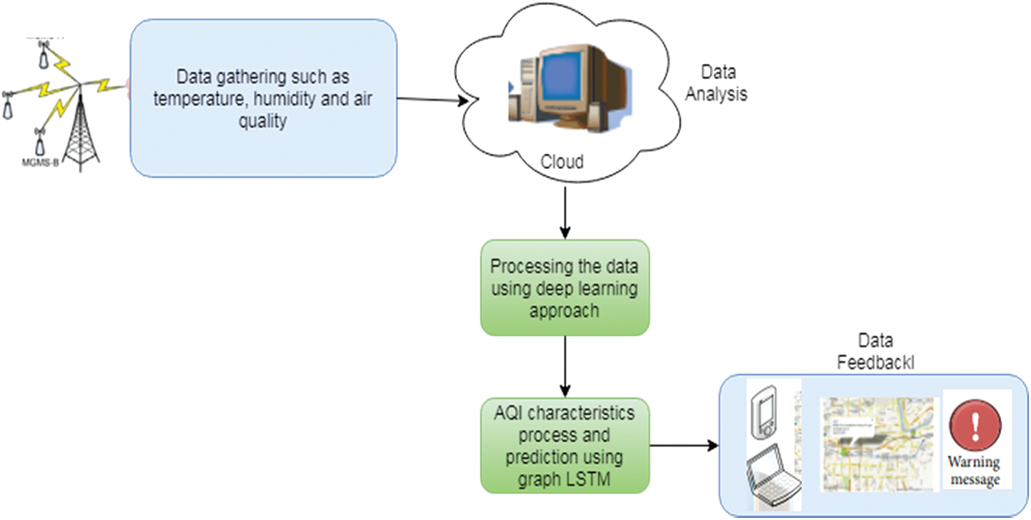
Figure 1: Proposed system overview
3.1 Data Gathering/Sensing Module
The data about the air quality such as temperature, humidity and AQI are gathered using the sensor nodes placed over that area. Each data gathering unit consists of array of sensors/IoT devices that measure various pollutants. The Data gather unit is designed with the wireless module to transfer the measurements through the general packet radio service (GPRS). This module can monitor the pollutant such as Nitrogen di oxide (NO2), Carbon di oxide (CO2), Carbon Monoxide (CO), ground level ozone (O3) and also relative humidity and temperature. New sensor station can also be added to monitor the Sulfur Dioxyde (SO2), Nitorgen oxide (NO) with Particulate Matter (PM). It can also be used to measure the wind speed and direction.
3.2 Data Analysis and Networking Module
This data analysis module is the link between the sensing module and backend processing module. This will provide the interface to extract the relevant data from the gathered data. The dataset used in this work is divided into three parts such as pollutants such as CO, CO2, NO2, PM, O3, locations of the GPS with latitude and longitude and time stamp such as data and time. The researchers used the AQI to measure the pollutants. AQI is the color-coded unit less index that is used to communicate the air quality concentration effective. The AQI computation of the particular air pollutant is based on average time period acquired from sensing PM. The risk of classification metrics in air pollutant is considered if its range is 0–300 and above. The coefficients of AQI metric are computed as Eq. (1).
where,
Pavg-average measurement of the concentration for last 24 hrs in mg/m3
Pmax-maximum concentration of the certain pollutant with risk classification metric
Pmin-minimum concentration of the certain pollutant with risk classification metric
AQImax-maximum AQI value of the certain pollutant with risk classification metric
AQImin-minimum AQI value of certain pollutant with risk classification metric
The AQI of the gathered pollutant are calculated from Eq. (1) which are independent. The gathered need to be preprocessed to handle the missing values. In this proposed work, portable web publication (PWP) dataset has been used for analysis which consist of 189648 samples with 18 features. This model has been trained with 60000 samples and the remaining instances are considered for testing. In the dataset, the dependent and independent features of the air quantities are identified. During this data preprocessing stage, among the 18 features, 12 features are selected for the prediction of air quality using the proposed dual graph convolutional network.
3.3 Air Pollutant Prediction Using Proposed Model
In this proposed work, the hybridization of two methods such as dual graph convolution network (DGCN) and graph LSTM has been to use to predict and monitoring the air quality. Here, the DGCN has been used to select the air pollutant features efficiently for the intelligent monitoring. GLSTM has been used to learn the AQI characteristics with information transfer with the feedback about the quality of the air and alert the environmental users. Parallel computing of various air data from sensor/IoT devices to centralized storage makes GPRS to compute data efficiently.
3.3.1 Dual Graph Convolutional Neural Network
The graph based neural network concept was first to propose that extension of existing neural network with graph domains. In graph, each node can be represented using features and related nodes. This dual graph convolutional network is considered as local and global graph consistency. The two convolutional neural networks are used to capture both local and global graph consistency. In the DGCN, the data set is denoted as a matrix X ∈ Rn×k and the set of data points are represented as X = {x1, x2,..xi, xi+1, …xn} and the graph structure. The label for the first i points are represented as y = {y1, y2, …yl}. The graph structure is represented as an adjacency matrix A ∈ Rn×n. The DGCN is formed with local consistency convolutional, global consistency convolutional and ensemble.
Local consistency of graph structured convolution convLC is a kind of feed forward network. The input is given to this model are feature matrix as X and adjacency matrix as A. The hidden output layer i of the local convolutional layer Z is declared in Eq. (2),
where,
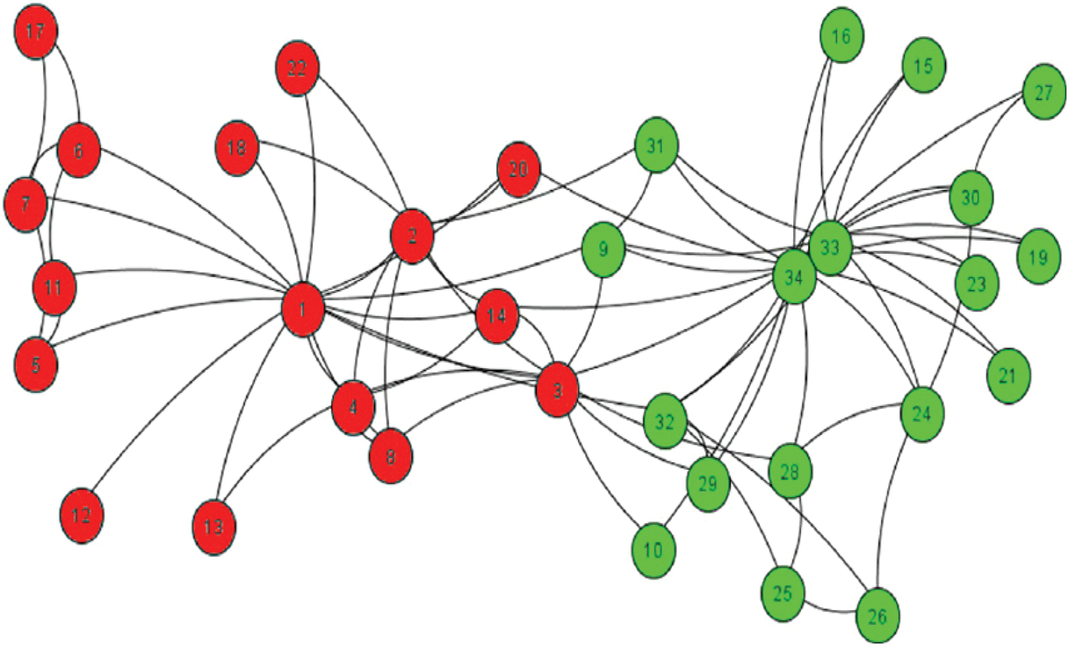
Figure 2: Karate club network for local consistency convolution
Global consistency convolution (G) is formed with the PPMI for encoding the information and it is denoted as G ∈ Rn×n. Initially the frequency matrix (FM) is calculated for a path chosen as random. FM can be used to calculate the G. This G based global convolution is represented as convGC.
The frequency matrix FM is calculated as follows: The random path is chosen by using node sequence visited by the user randomly. If the user on the node xi are random at time t, the state described as s(t) = xi. The node transfer from one node to the neighbor xj is declared as, r(s(t + 1) = xjs(t) = xi). These transition states are assigned to the given adjacency matrix A as Eq. (3). Random walk used here for similarity calculation between the nodes.
The frequency matrix FM is created using the Eq. (3) for all the pairs of nodes. The path between the nodes is calculated using random walk. Once the FM is created, the ith node of FM is the ith row vector of FMi and jth column of FM is the jth column vector of FMj. It is also called as context cj. The entry of the frequency matrix FMi,j is the number of time xi occurs in cj. Then the FM has been used to calculate matrix as PPMI where P ∈ Rn×n as in the Eqs. (4) to (8).
where,
Pi,j-probability of node xi occurs in context cj
Pi,*-probability of node xi
P*,j-probability of context cj
Compared to the adjacency matrix, PPMI matrix has reduced the hub nodes and increate the relationship among the data points. The global consistency convolution network convG based on the PPMI matrix is denoted in Eq. (9).
where,
P-PPMI matrix and
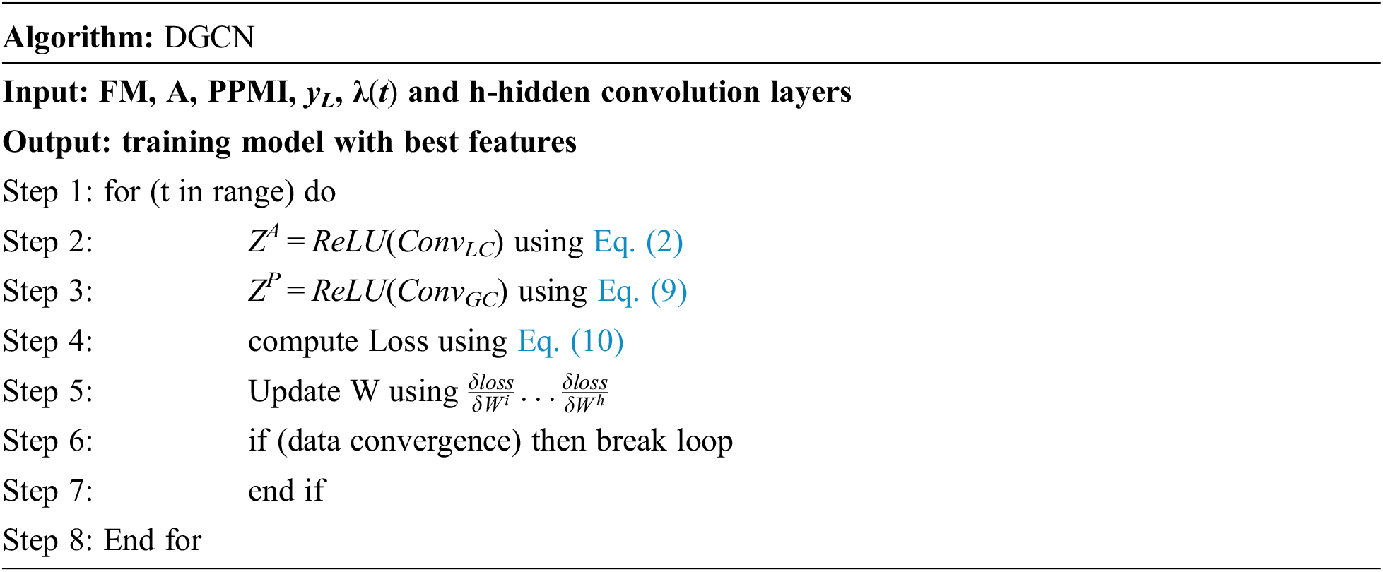
The local and global consistency are combined using convolution for dual graph convolutional network, regularizer used. Loss function with this regularizer is represented in Eq. (10)
where yL–labelled data for tranining and Y ∈ Rn×n
For both L0(Conv LC) and Lreg(Conv LC, Conv GC) calculation the activation function called ReLU has been used. After applying the activation function on Eqs. (11) and (12), the output matrix is represented as ZA ∈ Rn×c and ZP ∈ Rn×c respectively. The structure of dual graph convolutional network is shown in Fig. 3.
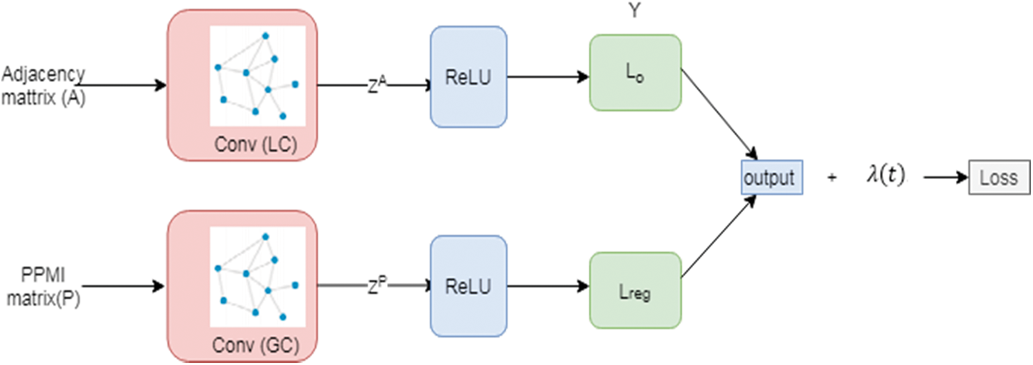
Figure 3: DGCN
3.3.2 Graph Structured LSTM Neural Network
In this proposed work G-LSTM has been used to train and learn the characteristics of the air pollutant for air quality monitoring. LSTM is a kind of recurrent neural network used to predict the events with long delay and time interval [21]. Compared to traditional LSTM, in graph LSTM each tree node represents the single unit of LSTM. In one direction of the graph, the node history is captured and, in another direction, the response for that comment is characterized. For the input ‘xt’ which have both text comments and submission context with hierarchical and timing layer. The node state transition are represented as a vector using the standard LSTM [22]. Fig. 4 shows the hierarchical and timing structure of Graph LSTM that are contributed to time.
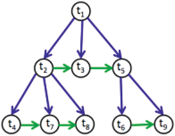
Figure 4: Forward G-LSTM hierarchical and timing structure
The graph is characterized as follows: let P(t) is the parent of node t and k(t) is the first node of child. The structure of timing is represented with the siblings: The predecessor p(t) and the successors (t) of the sibling. When t has no child, no predecessor, or no successor, then the pointers such as k(t), p(t) and s(t) are set as null. For the forward hierarchical LSTM, the equations are updated with the parameters such as, input gate i, temporal forget gate f, hierarchical forget gate h, cell c and output o respectively. The vectors such as it, ft and ht are used. Where,
it-new information weights
ft-siblings old data are remembered
ht-parent old data are remembered
σ-sigmoid function
Based on these parameters the equations are updated as follows from Eqs. (13) to (17),
For the backward LSTM the equations update are same apart from that the first child which passes the hidden state to its parents. π(t) is replace with k(t) and p(t) is replace with s(t) for backward graph LSTM which is represented in Fig. 5 and from Eqs. (18) to (22)
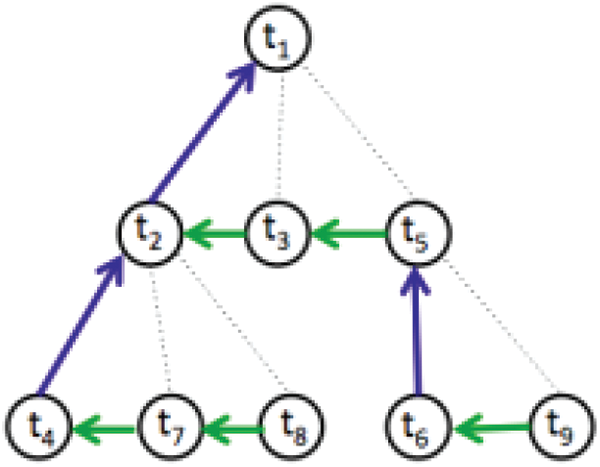
Figure 5: Backward graph LSTM with hierarchical and timing structure
Fig. 6 shows the proposed combined architecture of dual graph convolutional and G-LSTM network. Here the G-LSTM network with DGCN has been introduced to process the long-term data in a timely way that can utilize the raw information and predict the air pollutant quality in an efficient way.
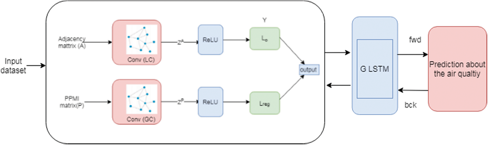
Figure 6: Combined fusion of proposed dual graph convolutional and G-LSTM network
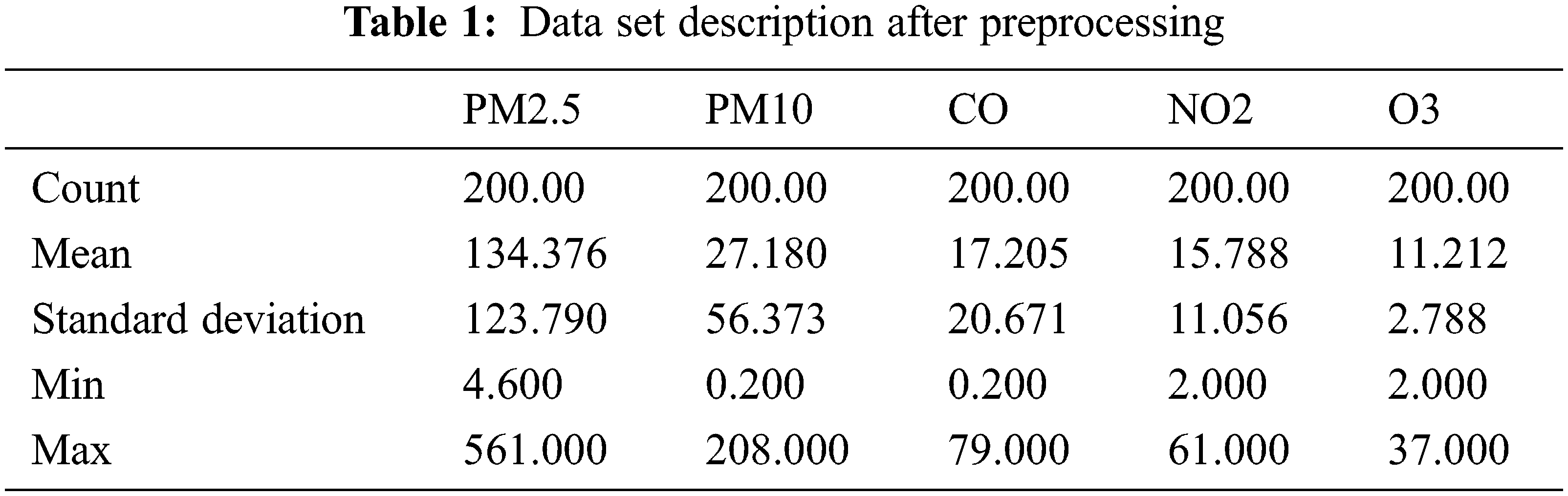
The experimental analysis of our proposed smart air pollution prediction environment has been tested using the data from the PWP which contains the name of 35 stations with air pollutant concentration such as PM2.5, PM10, CO, NO2 and O3. The raw dataset having missing values which are not normalized. During the first phase of our proposed work called data gathering, the raw data is preprocessed to get normalized data [23]. The normalized data set is shown in Tab. 1. The algorithms are implanted using python programming. The preprocessing stage is done by panda. The evaluation metrics are calculated using sklearn in python.
To evaluate the proposed work with the simulation data set, the error among actual and predicted values is calculated using various error measuring such as Mean Absolute Error (MAE), Root Mean Square Error (RMSE) and accuracy. Mean Absolute Error (MAE) is average magnitude measures of the errors in the set of predictions. It is the measure of the difference between the values of actual and predicted using the Eq. (23). Root Mean Square Error (RMSE) is the measurement of the average of the squared differences between values of actual and predicted value using the Eq. (24)
n-number of observations, yj-actual value,
The performance evaluation of the proposed air quality monitoring system is compared with the existing approaches such as linear regression (LR) based air quality prediction and artificial neural network (ANN) based air quality prediction system from paper [24–27]. The accuracy comparison is shown in Tab. 2.
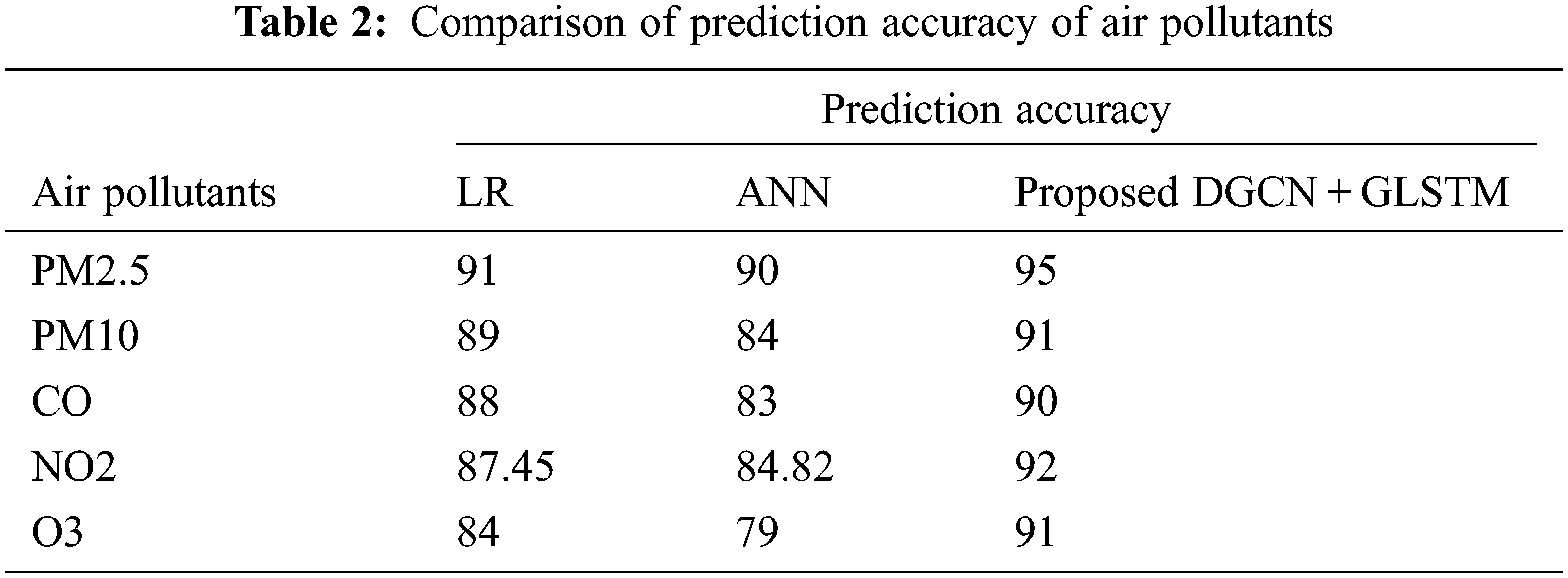
The observed results from Fig. 7 indicate pollutant of the PM 2.5 accuracy was highly recorded when compared to other pollutants of air. For further air pollutants the accuracy recorded was lesser than the basic level. And the comparative analysis proves that the proposed Dual graph convolutional with GLSTM method performs better than other approaches with high accuracy in the range of 90% to 95%. The other two methods such as LR and ANN obtains 84%–91% and 79%–90% respectively which is lower than proposed algorithm. Hence in terms of predicting the air pollutant level, our proposed algorithm outperforms. The comparative analysis in terms of MSE and RMSE is shown in Tab. 3.
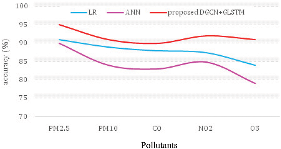
Figure 7: Air pollutant prediction accuracy of various algorithms
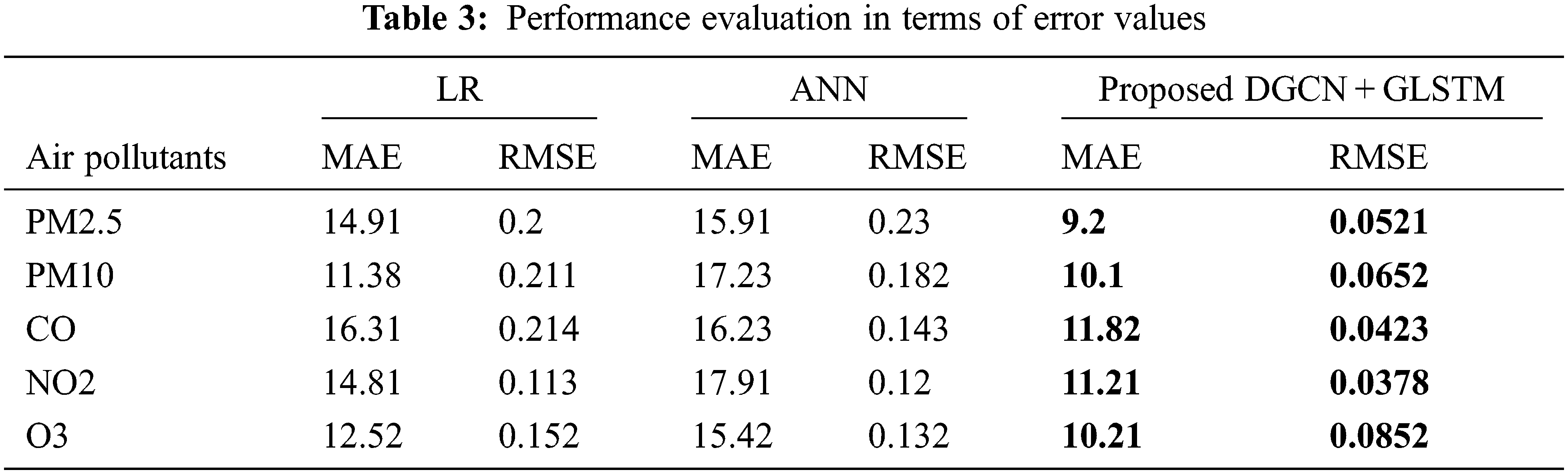
It can be observed red Figs. 8 and 9 that the obtained error rate for the proposed method records the minimal mean squared error and root mean squared error which are around 9–10 and 0.03–0.08 respectively. Furthermore, the remaining two methods such as LR and ANN obtains higher level of error rate than the proposed method for air pollutants like PM2.5, PM10, NO2, CO and O3. Hence proposed system proves as intelligent technology to monitor the air quality services.
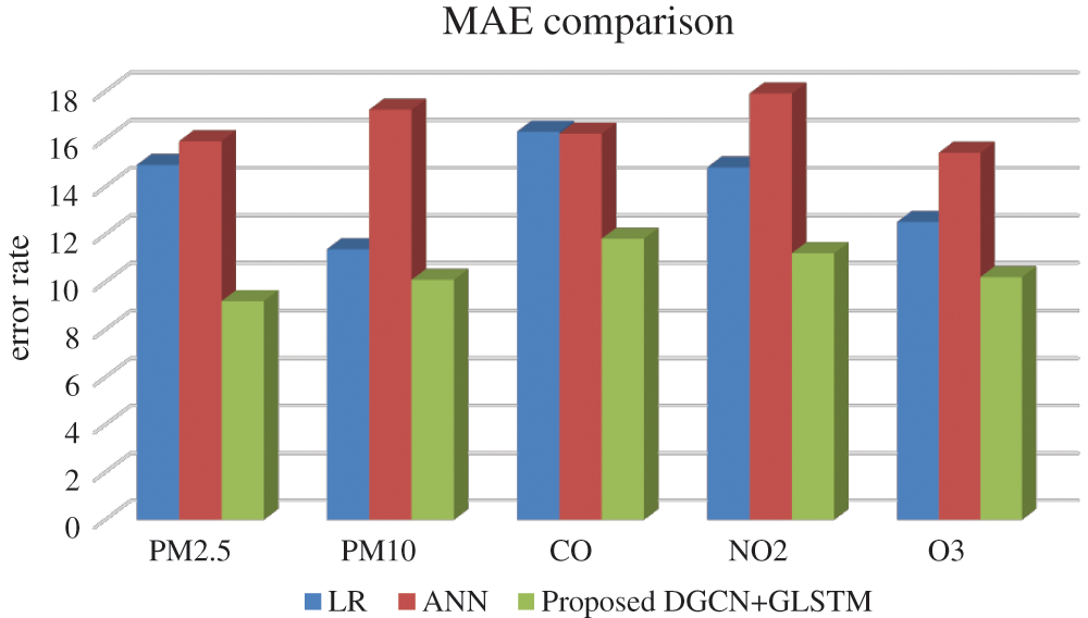
Figure 8: MAE comparison
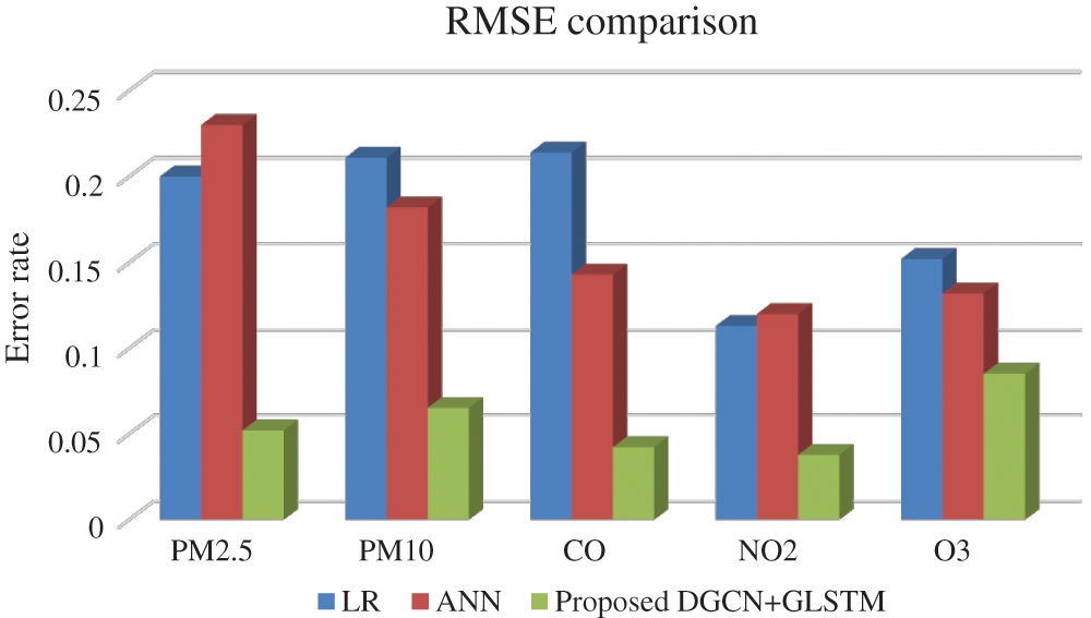
Figure 9: RMSE comparison
Air pollution is everything that causes hazards to human life. Human cannot survey without air (Oxygen). But in reality, the air is mixture of many particles and gases. When we inhale harmful particles enter body via respiratory tract and causes immunity problems. In this research work we use deep learning model to alert the human population regarding their surrounding air quality. Graph convolutional neural network with graph LSTM helps to adjudge the presence of pollutants with high accuracy. Hence, in terms of prediction accuracy and error rate, our proposed graph convolutional based LSTM performs efficiently on sending feedback about the air quality and proven to be the intelligent air quality monitoring system. Accuracy of proposed model reaches 95% in measuring the pollutant levels. This system can be studied and enhanced using some hybrid machine learning algorithm to bring the higher accuracy in future research work.
Acknowledgement: We would like to give special thanks to Taif University Researchers supporting project number (TURSP-2020/10), Taif University, Taif, Saudi Arabia.
Funding Statement: Taif University Researchers supporting project number (TURSP-2020/10), Taif University, Taif, Saudi Arabia.
Conflicts of Interest: The authors declare that they have no conflicts of interest to report regarding the present study.
1. Airnow, “Air Quality Index Basics,” 2020. [Online]. Available: https://www.airnow.gov/aqi/aqi-basics. [Google Scholar]
2. S. Pandya, H. Ghayvat, A. Sur, M. Awais, K. Kotecha et al., “Pollution weather prediction system: Smart outdoor pollution monitoring and prediction for healthy breathing and living,” Sensors, vol. 20, no. 18, pp. 5448, 2020. [Google Scholar]
3. H. Ly, L. M. Le, L. V. Phi, V. H. Phan, V. Tran et al., “Development of an AI model to measure traffic air pollution from multisensor and weather data,” Sensors, vol. 19, no. 22, pp. 4941, 2019. [Google Scholar]
4. T. C. Yu and C. C. Lin, “An intelligent wireless sensing and control system to improve indoor air quality: Monitoring, prediction, and preaction,” International Journal of Distributed Sensor Networks, vol. 11, no. 8, pp. 140978, 2015. [Google Scholar]
5. N. Salman, A. H. Kemp, A. Khan and C. Noakes, “Real time wireless sensor network (WSN) based indoor air quality monitoring system,” IFAC-PapersOnLine, vol. 52, no. 24, pp. 324–327, 2019. [Google Scholar]
6. E. Yaacoub, A. Kadri, M. Mushtaha and A. Abudayya, “Air quality monitoring and analysis in Qatar using a wireless sensor network deployment,” in Proc. IWCMC, Sardinia, Italy, pp. 596–601, 2013. [Google Scholar]
7. J. Zhou, G. Cui, S. Hu, Z. Zhang, C. Yang et al., “Graph neural networks: A review of methods and applications,” AI Open, vol. 1, pp. 57–81, 2020. [Google Scholar]
8. W. Jiang, Y. Wang, M. H. T. Sou and X. Fu, “Using social media to detect outdoor air pollution and monitor air quality index (AQIA geo-targeted spatiotemporal analysis framework with Sina Weibo (Chinese Twitter),” PLoS One, vol. 10, no. 10, pp. e0141185, 2015. [Google Scholar]
9. E. G. Dragomir, “Air quality index prediction using K-nearest neighbor technique,” Bulletin of PG University of Ploiesti, Series Mathematics, Informatics, Physics, LXII, vol. 1, no. 2010, pp. 103–108, 2010. [Google Scholar]
10. C. Suo, Y. Li, J. Sun and S. Yin, “An air quality index-based multistage type-2-fuzzy interval-stochastic programming model for energy and environmental systems management under multiple uncertainties,” Environmental Research, vol. 167, pp. 98–114, 2018. [Google Scholar]
11. M. Richards, M. Ghanem, M. Osmond, Y. Guo and J. Hassard, “Grid-based analysis of air pollution data,” Ecological Modelling, vol. 194, no. 1–3, pp. 274–286, 2006. [Google Scholar]
12. S. Dhingra, R. B. Madda, A. H. Gandomi, R. Patan and M. Daneshmand, “Internet of things mobileair pollution monitoring system (IoT-Mobair),” IEEE Internet of Things Journal, vol. 6, no. 3, pp. 5577–5584, 2019. [Google Scholar]
13. R. K. Grace and S. Manju, “A comprehensive review of wireless sensor networks based air pollution monitoring systems,” Wireless Personal Communications, vol. 108, no. 4, pp. 2499–2515, 2019. [Google Scholar]
14. K. K. Khedo and V. Chikhooreeah, “Low-cost energy-efficient air quality monitoring system using wireless sensor network,” Wireless Sensor Networks-Insights and Innovations, InTech, vol. 12, no. 5, pp. 121–140, 2017. [Google Scholar]
15. J. Saini, M. Dutta and G. Marques, “A comprehensive review on indoor air quality monitoring systems for enhanced public health,” Sustainable Environment Research, vol. 30, no. 1, pp. 1–12, 2020. [Google Scholar]
16. R. S. Ram, M. V. Kumar, S. Ramamoorthy, B. S. Balaji and T. R. Kumar, “An efficient hybrid computing environment to develop a confidential and authenticated IoT service model,” Wireless Personal Communications, vol. 117, no. 4, pp. 2903–2927, 2021. [Google Scholar]
17. M. V. Kumar, R. S. Ram, B. Amutha and M. Kowsigan, “An improved migration scheme to achieve the optimal service time for the active jobs in 5G cloud environment,” Computer Communications, vol. 160, pp. 807–814, 2020. [Google Scholar]
18. S. R. Ram, B. Subramanian, N. Bacanin, M. Zivkovic and I. Strumberger, “Speech enhancement through improvised conditional generative adversarial networks,” Microprocessors and Microsystems, vol. 79, pp. 103281, 2020. [Google Scholar]
19. R. S. Ram, A. G. Saminathan and S. A. Prakash, “An area efficient and low power consumption of run time digital system based on dynamic partial reconfiguration,” International Journal of Parallel Programming, vol. 48, no. 3, pp. 431–446, 2020. [Google Scholar]
20. R. S. Ram, S. A. Prakash, M. Balaanand and C. Sivaparthipan, “Colour and orientation of pixel based video retrieval using IHBM similarity measure,” Multimedia Tools and Applications, vol. 79, no. 15, pp. 10199–10214, 2020. [Google Scholar]
21. T. N. Kipf and M. Welling, “Semi-supervised classification with graph convolutional networks,” Published as a conference paper at ICLR 2017, Toulon, France, pp. 1–14, 2017. [Google Scholar]
22. L. Van der Maaten and G. Hinton, “Visualizing data using t-SNE,” Journal of Machine Learning Research, vol. 9, no. 11, pp. 2579–2605, 2008. [Google Scholar]
23. T. Fischer and C. Krauss, “Deep learning with long short-term memory networks for financial market predictions,” European Journal of Operational Research, vol. 270, no. 2, pp. 654–669, 2018. [Google Scholar]
24. J. Zhou, J. Xiang and S. Huang, “Classification and prediction of typhoon levels by satellite cloud pictures through GC–LSTM deep learning model,” Sensors, vol. 20, no. 18, pp. 5132, 2020. [Google Scholar]
25. S. Al-Janabi, M. Mohammad and A. Al-Sultan, “A new method for prediction of air pollution based on intelligent computation,” Soft Computing, vol. 24, no. 1, pp. 661–680, 2020. [Google Scholar]
26. S. Mahajan, A. Raina, M. Abouhawwash, X. Gao and A. K. Pandit, “Covid-19 detection from chest X-Ray images using advanced deep learning techniques,” Computers, Materials and Continua, vol. 70, no. 1, pp. 1541–1556, 2022. [Google Scholar]
27. V. Kandasamy, P. Trojovský, F. Machot, K. Kyamakya, N. Bacanin et al., “Sentimental analysis of COVID-19 related messages in social networks by involving an N-gram stacked autoencoder integrated in an ensemble learning scheme,” Sensors, vol. 21, no. 22, pp. 7582, 2021. [Google Scholar]
 | This work is licensed under a Creative Commons Attribution 4.0 International License, which permits unrestricted use, distribution, and reproduction in any medium, provided the original work is properly cited. |