DOI:10.32604/iasc.2022.017049
| Intelligent Automation & Soft Computing DOI:10.32604/iasc.2022.017049 | |
| Article |
Sensor Location Optimisation Design Based on IoT and Geostatistics in Greenhouse
1Information Center, Jiangsu Academy of Agricultural Sciences, Nanjing, 210014, China
2Jiangsu Vocational College of Agriculture and Forestry, Jurong, 212400, China
3Key Laboratory of Agro-Environment in Downstream of Yangtze Plain, Ministry of Agriculture and Rural Affairs/Institute of Agricultural Resources and Environment, Jiangsu Academy of Agricultural Sciences, Nanjing, 210014, China
4U. S. National Poultry Research Center, Agricultural Research Service, United States Department of Agriculture, Athens, GA 30605, USA
*Corresponding Author: Ni Ren. Email: rn@jaas.ac.cn
Received: 19 January 2021; Accepted: 05 January 2022
Abstract: Environmental parameters such as air temperature (T) and air relative humidity (RH) should be intensively monitored in a greenhouse in real time. In most cases, one set of sensors is installed in the centre of a greenhouse. However, as the microclimate of a greenhouse is always heterogeneous, the sensor installation location is crucial for practical cultivation. In this study, the T and RH monitoring performance of different sensors were compared. Two types of real-time environmental sensors (Air Temperature and Humidity sensor and Activity Monitoring sensor, referred as ATH and AM) were selected and calibrated by reliable non-real-time sensors (Honest Observer By Onset sensor, referred as HOBO). The results showed that T and RH were variable in a small greenhouse area (128 m2). ATH had better T and RH monitoring performance than AM using HOBO as a reference (R2 = 0.968 and 0.938 for T; 0.594 and 0.538 for RH, respectively, for ATH and AM). In terms of cost, it is more efficient to use more sets of AMs (15 sets were used in this case study) to establish an intensive monitoring system based on the Internet of Things (IoT) compared with that of ATH. Then, the optimal sensor installation location was decided using geostatistics. Based on a simulated monitoring data set, the optimal sensor installation location was determined to be 1.57 m away from the physical centre of the monitoring area. By combining IoT with geostatistics, this study offers a method for effective monitoring of environmental parameters in a practical greenhouse system with a three-step procedure.
Keywords: Vegetable greenhouse; environmental monitoring; internet of things; sensor location design; ordinary kriging
In traditional greenhouse facilities, intensive fertilisation and irrigation are required for maximising profits [1]. However, excessive fertilisation and irrigation may increase cultivation cost and cause environmental problems such as nutrient leaching and secondary salinisation [2,3]. Hence, a greenhouse requires precision cultivation which focused on providing information for observing, assessing and managing agricultural practices [4]. Precision agriculture is targeted to maximise productivity and minimise the use of fertilisers [5], thereby achieving efficient, green and sustainable agriculture [6,7]. A feasible solution for precision agriculture can be a monitoring system based on environmental sensors [8] aimed to collect environmental data, which can be analysed to optimise the management [9]. Air temperature (T) and air relative humidity (RH) are the main environmental parameters affecting plant growth [10]. In a greenhouse system, T is generally maintained at 20°C–30°C, and RH at 60%–90% [11]. Continuous environmental monitoring of a greenhouse can provide information on the effect of fluctuating factors on plant growth and how to increase greenhouse production by microclimate adjustment [8].
Most previous research assumed a more uniform climate condition in a greenhouse system than an open field [12,13]. However, several studies detected the heterogeneity of greenhouse environmental conditions such as T, RH and daily reference evapotranspiration [11,14]. The results based on the measurements by Ferentinos et al. [15] demonstrated considerable microclimate spatial variability in a greenhouse. The average differences could reach 3.3°C and 9% (within 160 m2) for T and RH, respectively. Climatic heterogeneity can cause variability in the production and quality of plants [15]. Spatially distributed environmental measurements can provide precise and specific data of the heterogeneous greenhouse climate [4]. With the development of the Internet of Things (IoT), wireless real-time environmental sensor nodes with a large transmit range are preferred compared with wired ones in modern greenhouse systems [16,17]. For example, Li et al. [9] adopted a digital thermometer DS18B20 and a single RH sensor AM2001 to remotely monitor environmental information in a greenhouse system. Based on SHT75, Chang et al. [18] designed a greenhouse environmental monitoring system to measure T and RH. Park et al. [19] also contributed to improving productivity and preventing crops from blight and infestation by insects by using T and RH sensors.
To be specific, a monitoring system requires not only intensive temporal and spatial data but also reliability. Moreover, environmental monitoring systems should be affordable to farmers [20]. The accuracy and hardware cost are key factors for practical sensor selection. Until recent years, intensive distributed sensors have been expensive and less user-friendly for farmers training or expertise to handle such sensors. It is more feasible to use one set of sensors to monitor greenhouses. Consequently, the installation locations of sensors should be representative for an entire greenhouse area. Geostatistical methods such as kriging have been rapidly developing in the past decades [21]. The basis of geostatistical estimation is the assumption that an observation of a variable ‘z’ at location ‘s’ was a realisation of a random field ‘Z(s)’ [22]. This method has been widely used in agricultural and environmental research at a large scale [23]. Unlike the large-scale methodologies used in previous studies, in the present study, the geostatistical method has been introduced to calculate the optimal installation locations of sensors at a small scale, thereby improving the cost-effectiveness.
For a practical monitoring system, the basis for comparison should be selection of suitable sensors, and optimisation of sensor installation locations. To the best of our knowledge, limited studies have addressed the costs, accuracy and locations of environmental sensors in a greenhouse system. In the present study, three environmental sensors were selected to (1) compare the variations of T and RH at different sites in the greenhouse; (2) compare the accuracy of different sensors; and (3) estimate the optimal location of the sensor for efficiency. The results can offer an appropriate design of environmental monitoring system under greenhouse conditions to maximise productivity with cost-effectiveness.
Three types of sensors were used in the present study: HOBO U23-001 (non-real-time, Onset Computer Corporation, Bourne, MA, USA), ATH-2z (real-time, Bio Instruments, Chisinau, Moldova), and AM2322 (real-time, ASAIR, Guangzhou, China), hereafter referred to as HOBO, ATH and AM (Honest Observer By Onset sensor, Air Temperature and Humidity sensor and Activity Monitoring sensor), with the information listed in Tab. 1.
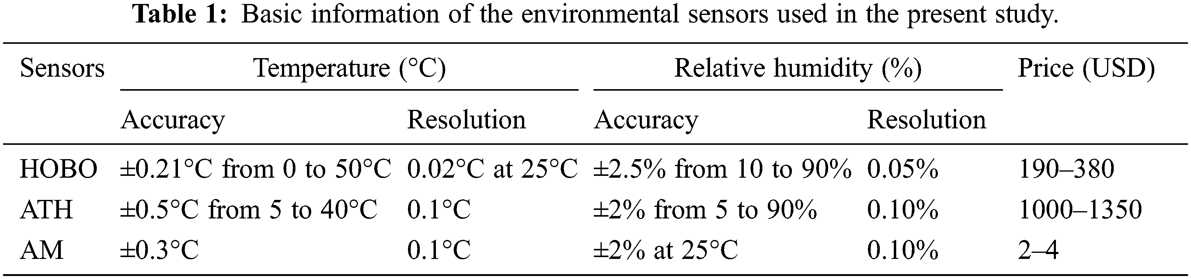
HOBO can measure T from −40°C to 70°C and RH from 0 to 100%, with widespread agricultural applications. Considering its popularity and intensive uses in industrial and scientific purposes, the present study used HOBO as a reference for the other two real-time sensors (ATH and AM). ATH is power aspirated and could transmit data through real-time networks. Located inside a protective enclosure, the integrated T and RH sensor can measure T from 0°C to 50°C and RH from 0 to 100%. AM can measure T from −40°C to 80°C and RH from 0 to 99.9%. All the sensors in the present study were calibrated by their manufacturing companies within six months.
2.2 Experimental Site and Design
The study was conducted in a Venlo-type glass greenhouse (PRIVA, De Lier, Netherland) in Jiangsu Academy of Agricultural Sciences, Nanjing, Jiangsu Province, China (32°02′10.4″N, 118°52′14.9″E). The greenhouse for tomato cultivation was 6 m high with an area of approximately 960 m2 (24 m × 40 m), and divided into six sections as shown in Fig. 1. For heat preservation, an extra polyethylene film was installed inside the greenhouse at 2.2 m.

Figure 1: Locations of environmental sensors installed in the greenhouse
Before installed in the greenhouse, two HOBO sensors were calibrated in a laboratory (around 11°C). Both sensors were located within 10 cm for 48 h, and T and RH were recorded at an interval of 10 min. A total of 288 observations were recorded, and the latter 144 records were used for calibration.
Fig. 1 shows the locations of two real-time sensors, ATH and AM. Two calibrated HOBO sensors were installed within 40 cm as HOBO-ATH and HOBO-AM. All four sensors were installed at 1.8 m on Feb. 26, 2019 (the recording interval was 10 min). After installation, observations of the first 24 h were excluded for measurement stabilisation. A total of 144 records (Feb. 27–28, 2019) were used for comparison of sensor performances.
2.3 Spatial Interpolation and Statistical Analysis
Ordinary kriging was applied to spatially interpolate T to study its spatial distribution in the greenhouse and to represent spatial heterogeneity [24,25]. It quantified the spatial variation of a regionalisation variable with the semivariogram (Eq. (1)). This procedure was used considering that it provides the best unbiased linear estimation for an unknown point [21,26].
where
In this simulated research, a grid distribution (4 m × 4 m) of AM was assumed in the 8 m × 16 m greenhouse section (Fig. 1). The values were randomly selected from T observed from AM (due to the shortage of grid distributed electricity, simulated research was applied to replace practical measurement). The spatial interpolation was conducted with ArcGIS 10.0. Linear regression analysis was performed to determine the relationships of T and RH between different sensors and p < 0.05 was used as the standard for significance. The mean absolute error (MAE) and the root-mean-square error (RMSE) were calculated as follows:
where
3.1 Calibration of HOBO Sensors
Calibration results showed that T from two HOBO sensors were in good accordance, with an MAE and RMSE at 0.03°C and 0.04°C, respectively (Tab. 2). However, the variability of RH was larger than that of T, with an MAE and RMSE at 0.42 and 0.50% (Tab. 2). T and RH from the two HOBO sensors were significantly correlated (p < 0.001). R2 of T and RH were 0.986 and 0.782 (Fig. 2). The calibration results indicated that both sensors were well-calibrated before use as references in the greenhouse.
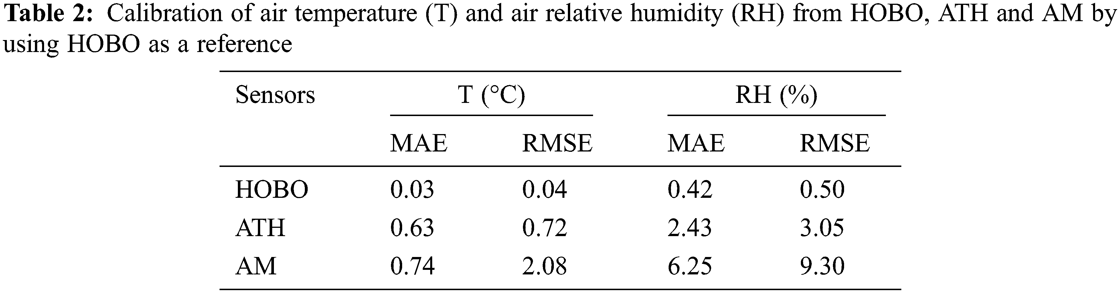

Figure 2: Linear regression of air temperature and air relative humidity observed by two HOBO sensors in the laboratory before their installation in the greenhouse. The solid line is the fitting line of linear regression, and the dashed line is the 1:1 line
3.2 Comparison of T and RH from ATH and AM
The comparison between different locations of the greenhouse showed that HOBO-ATH had a higher T (+1.57°C) and a lower RH (−8.23%) than HOBO-AM. The results demonstrated that environmental parameters were different in a small section of the greenhouse. As a result, the installation location should be optimised when only one set of environmental sensors is available. Using HOBO as a reference, high MAE and RMSE were observed from two real-time sensors for T and RH (Tab. 2). ATH performed better than AM; RMSE of T and RH from AM increased by 188.89% and 204.92%, respectively, compared with that from ATH.
The regression analysis further demonstrated that ATH performed better than AM for T and RH monitoring (Fig. 3). In terms of T observation, ATH and AM showed good fitting results based on the reference of HOBO (R2 = 0.968 and 0.938 for ATH and AM, respectively). In terms of RH observation, ATH showed better fitting results than AM (R2 = 0.594 and 0.538 for ATH and AM, respectively). The results indicated that T observation was reliable for all three kinds of sensors. However, RH observation was not stable even between the same type of sensors (Tab. 2). Hence, reliable sensors were required to obtain precise RH monitoring.

Figure 3: Linear regression between air temperature and air relative humidity observed by ATH and AM compared with HOBO in the greenhouse. The solid line is the fitting line of linear regression, the dashed line is the 1:1 line
4.1 Sensor Selection for Greenhouse Monitoring System
In the present study, data from various sensors showed different T and RH data even in a small greenhouse section. Consequently, a system with a reasonable sensor installation location should be designed for accurate monitoring [27]. Compared with AM, ATH was more accurate for T and RH monitoring, but with a much higher cost. For practical greenhouse cultivation, sensor costs are a limiting factor, especially when many sensors are required for a holistic approach to environmental monitoring [28]. AM sensors cost less than ATH and have great potential for establishing a real-time monitoring system based on IoT.
A sensor comparison showed that T could be monitored by AM rather than ATH without introducing large uncertainty. However, RH measured by different sensors was variable. Based on the reference of HOBO, ATH performed better compared with AM (Tab. 2). The results indicated that ATH or HOBO was more reliable and could not be replaced by AM.
T and RH were always negatively correlated [29]. In the present study, T and RH observed from ATH and AM also showed a significant negative correlation (R2 = 0.721 and 0.791, respectively) (Fig. 4), indicating that T monitoring could be used as an indicator of RH.
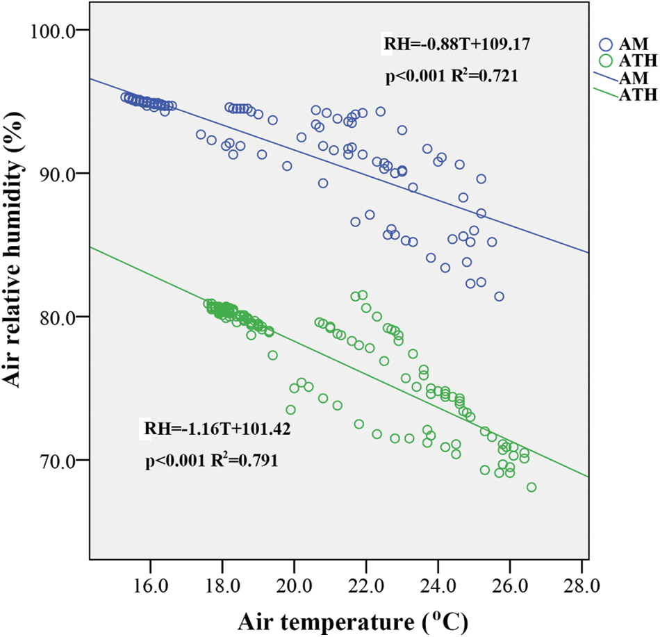
Figure 4: Relationship between air temperature (T) and air relative humidity (RH) observed from ATH and AM
4.2 Air Relative Humidity Monitoring
Greenhouse cultivation requires sufficient irrigation [3], because excessive irrigation increases the RH [30]. In winter, the enclosed greenhouse system benefitted from heat preservation, but air exchange was limited and RH could not drop in a short time [31]. Because of the high RH, the tomato and cucumber plants under greenhouse cultivation had a greater chance of suffering from severe diseases [32] such as grey mold disease (Botrytis cinerea Pers) [33] and blight (Phytophthora capsici sp. Leonina) [34]. RH should be carefully monitored and controlled to minimise yield loss from the diseases. However, the performance of different sensors showed that RH monitoring was varied. Accurate and stable RH monitoring sensors are scarcely affordable for practical production (over $1000 per set).
The uncertainty of RH monitoring from various sensors can be due to the high temporal and spatial variability of RH compared with T (Fig. 2) and the differences in solar radiation shields of sensors (Fig. 5). Before RH was measured, the fan would introduce fresh air into ATH. The impact of shields on the RH monitoring needs further investigation. Due to the high cost of reliable RH monitoring sensors, an optimal location should be designed to increase monitoring efficiency.
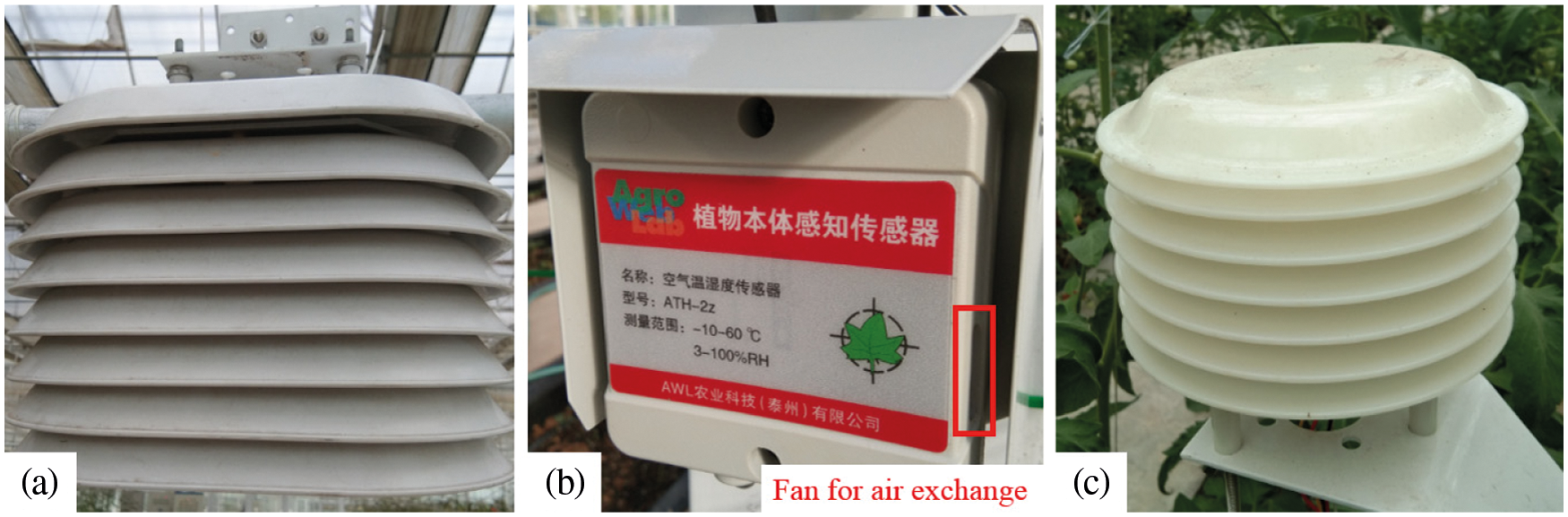
Figure 5: Different solar radiation shields for (a) HOBO, (b) ATH and (c) AM
Most monitoring systems locate sensors in the centre of the target, which is likely not the optimal location. It is more efficient to install sensors to represent the maximum area. Low-cost AM sensors were reliable for T monitoring, and could be intensively installed based on IoT techniques. For a case study, 15 AM sensors for a 4 × 4 m grid distribution were used to detect the variability of T (Fig. 6). For simulated research, ordinary kriging was conducted to show the spatial distribution of T in the greenhouse. The range of the variogram was 24 m.

Figure 6: Assumed ATH location based on air temperature monitoring from gird located AM
The average T of the greenhouse was calculated; the contour of spatial average T was obtained (20.6°C, the blue line in Fig. 6) and assumed to be the optimal location for T and RH monitoring. Compared with the centre of the monitoring area, the optimal location was offset by approximately 1.57 m. This simulated calculation showed that considerable distance might exist between the optimal sensor location and the centre of the monitoring area. A prior spatial calculation by using low-cost sensors based on IoT should, thus, be conducted before installation. In a future study, new techniques such as the Global Positioning System and artificial intelligence algorithms should be further introduced to facilitate the location design in greenhouse monitoring systems [17,35].
Briefly, the design of our monitoring system involved three steps: (1) interpolating the T from the grid located sensors and analysing the spatial variability; (2) calculating the contour of spatial average T; (3) determining the optimal sensor location, which was the point on the contour and was nearest to the centre of the greenhouse.
A greenhouse system has complicated microclimate conditions such as highly variable temporal and spatial air temperature and humidity. For practical greenhouse cultivation, cost, quality and location of environmental sensors should be considered. The results from the present study showed that air temperature monitoring was reliable for all three types of sensors (HOBO, ATH and AM), whereas air relative humidity monitoring was divergent. The optimal locations can be calculated to monitor the maximum area of a greenhouse based on IoT and geostatistical method accompanied with grid located sensors. Results from the present study provide a low cost and efficient environmental sensor design for a greenhouse system.
Funding Statement: This research was funded by the Key Research and Development Project of Jiangsu Province, Grant Number BE2021379; National Key Research and Development Program of China, Grant Number 2018YFD0800206; the Jiangsu Agricultural Science and Technology Innovation Fund, Grant Number CX(18)2029; the Foundation of Jiangsu Vocational College of Agriculture and Forestry (2019kj014).
Conflicts of Interest: The authors declare that they have no conflicts of interest to report regarding the present study.
1. H. Liang, H. Lv, W. D. Batchelor, X. Lian, Z. Wang et al., “Simulating nitrate and DON leaching to optimize water and N management practices for greenhouse vegetable production systems,” Agricultural Water Management, vol. 241, no. 1, pp. 106377, 2020. [Google Scholar]
2. W. M. Shi, J. Yao and F. Yan, “Vegetable cultivation under greenhouse conditions leads to rapid accumulation of nutrients, acidification and salinity of soils and groundwater contamination in South-Eastern China,” Nutrient Cycling in Agroecosystems, vol. 83, no. 1, pp. 73–84, 2009. [Google Scholar]
3. J. Li, H. Liu, H. Wang, J. Luo, X. Zhang et al., “Managing irrigation and fertilization for the sustainable cultivation of greenhouse vegetables,” Agricultural Water Management, vol. 210, pp. 354–363, 2018. [Google Scholar]
4. M. Mancuso and F. Bustaffa, “A wireless sensors network for monitoring environmental variables in a tomato greenhouse,” in 2006 IEEE Int. Workshop on Factory Communication Systems, Torino, pp. 107–110, 2006. [Google Scholar]
5. J. Muangprathub, N. Boonnam, S. Kajornkasirat, N. Lekbangpong, A. Wanichsombat et al., “IoT and agriculture data analysis for smart farm,” Computers and Electronics in Agriculture, vol. 156, no. 9, pp. 467–474, 2019. [Google Scholar]
6. T. Ojha, S. Misra and N. S. Raghuwanshi, “Wireless sensor networks for agriculture: The state-of-the-art in practice and future challenges,” Computers and Electronics in Agriculture, vol. 118, no. 4, pp. 66–84, 2015. [Google Scholar]
7. X. Feng, F. Yan and X. Liu, “Study of wireless communication technologies on internet of things for precision agriculture,” Wireless Personal Communications, vol. 108, no. 3, pp. 1785–1802, 2019. [Google Scholar]
8. S. Rodríguez, T. Gualotuña and C. Grilo, “A system for the monitoring and predicting of data in precision agriculture in a rose greenhouse based on wireless sensor networks,” Procedia Computer Science, vol. 121, no. 1, pp. 306–313, 2017. [Google Scholar]
9. S. L. Li, Y. Han, G. Li, M. Zhang, L. Zhang et al., “Design and implementation of agricultural greenhouse environmental monitoring system based on internet of things,” Applied Mechanics and Materials, vol. 121–126, pp. 2624–2629, 2012. [Google Scholar]
10. Y. H. Zhou and J. G. Duan, “Design and simulation of a wireless sensor network greenhouse-monitoring system based on 3G network communication,” International Journal of Online Engineering, vol. 12, no. 5, pp. 48, 2016. [Google Scholar]
11. S. R. Boselin Prabhu, C. V. Dhasharathi, R. Prabhakaran, M. Raj Kumar, S. Wasim Feroze et al., “Environmental monitoring and greenhouse control by distributed sensor network,” International Journal of Advanced Networking & Applications, vol. 5, no. 5, pp. 2060–2065, 2014. [Google Scholar]
12. C. R. Bojacá, R. Gil and A. Cooman, “Use of geostatistical and crop growth modelling to assess the variability of greenhouse tomato yield caused by spatial temperature variations,” Computers and Electronics in Agriculture, vol. 65, no. 2, pp. 219–227, 2009. [Google Scholar]
13. L. Vásquez, A. Iriarte, M. Almeida and P. Villalobos, “Evaluation of greenhouse gas emissions and proposals for their reduction at a university campus in Chile,” Journal of Cleaner Production, vol. 108, no. 1, pp. 924–930, 2015. [Google Scholar]
14. J. Yu, W. Zheng, L. Xu, L. Zhangzhong, G. Zhang et al., “A PSO-XGBoost model for estimating daily reference evapotranspiration in the solar greenhouse,” Intelligent Automation & Soft Computing, vol. 26, no. 5, pp. 989–1003, 2020. [Google Scholar]
15. K. P. Ferentinos, N. Katsoulas, A. Tzounis, T. Bartzanas and C. Kittas, “Wireless sensor networks for greenhouse climate and plant condition assessment,” Biosystems Engineering, vol. 153, no. 4, pp. 70–81, 2017. [Google Scholar]
16. M. E. Bayrakdar, “Cost effective smart system for water pollution control with underwater wireless sensor networks: A simulation study,” Computer Systems Science and Engineering, vol. 35, no. 4, pp. 283–292, 2020. [Google Scholar]
17. L. Wang, Z. Song, C. Huang, S. Jiang and J-H. Wang, “Special section on data-enabled intelligence in complex agricultural systems,” Intelligent Automation & Soft Computing, vol. 26, no. 5, pp. 947–948, 2020. [Google Scholar]
18. B. Chang, X. R. Zhang and L. H. Li, “Design of environment monitoring system based on can bus and wireless sensor networks for greenhouse,” Advanced Materials Research, vol. 1049–1050, pp. 1163–1166, 2014. [Google Scholar]
19. D. H. Park, B. J. Kang, K. R. Cho, C. S. Shin, S. E. Cho et al., “A study on greenhouse automatic control system based on wireless sensor network,” Wireless Personal Communications, vol. 56, no. 1, pp. 117–130, 2011. [Google Scholar]
20. A. Janarthanan and D. Kumar, “Localization based evolutionary routing (LOBER) for efficient aggregation in wireless multimedia sensor networks,” Computers, Materials and Continua, vol. 30, no. 3, pp. 895–912, 2019. [Google Scholar]
21. Z. Zhang, Y. Sun, D. Yu, P. Mao and L. Xu, “Influence of sampling point discretization on the regional variability of soil organic carbon in the red soil region, China,” Sustainability, vol. 10, no. 10, pp. 3603, 2018. [Google Scholar]
22. B. Minasny, J. A. Vrugt and A. B. McBratney, “Confronting uncertainty in model-based geostatistics using Markov Chain Monte Carlo simulation,” Geoderma, vol. 163, no. 3–4, pp. 150–162, 2011. [Google Scholar]
23. Y. Liu, D. Yu, N. Wang, X. Shi, E. D. Warner et al., “Impacts of agricultural intensity on soil organic carbon pools in a main vegetable cultivation region of China,” Soil and Tillage Research, vol. 134, no. 2, pp. 25–32, 2013. [Google Scholar]
24. U. Mishra, R. Lal, B. Slater, F. Calhoun, D. S. Liu et al., “Predicting soil organic carbon stock using profile depth distribution functions and ordinary kriging,” Soil Science Society of America Journal, vol. 73, no. 2, pp. 614–621, 2009. [Google Scholar]
25. D. S. Yu, H. Yang, X. Z. Shi, E. D. Warner, L. M. Zhang et al., “Effects of soil spatial resolution on quantifying CH4 and N2O emissions from rice fields in the Tai Lake region of China by DNDC model,” Global Biogeochemical Cycles, vol. 25, no. 2, pp. 1–8, 2011. [Google Scholar]
26. Z. Q. Zhang, D. S. Yu, X. Z. Shi, D. C. Weindorf, W. X. Sun et al., “Effects of prediction methods for detecting the temporal evolution of soil organic carbon in the Hilly Red Soil Region, China,” Environmental Earth Sciences, vol. 64, no. 2, pp. 319–328, 2011. [Google Scholar]
27. J. López-Martínez, J. L. Blanco-Claraco, J. Pérez-Alonso and Á.J. Callejón-Ferre, “Distributed network for measuring climatic parameters in heterogeneous environments: Application in a greenhouse,” Computers and Electronics in Agriculture, vol. 145, pp. 105–121, 2018. [Google Scholar]
28. D. Ma, N. Carpenter, H. Maki, T. U. Rehman, M. R. Tuinstra et al., “Greenhouse environment modeling and simulation for microclimate control,” Computers and Electronics in Agriculture, vol. 162, no. 4, pp. 134–142, 2019. [Google Scholar]
29. Z. Liu, J. Li, M. Liu, V. Cascioli and P. W. McCarthy, “In-depth investigation into the transient humidity response at the body-seat interface on initial contact using a dual temperature and humidity sensor,” Sensors, vol. 19, no. 6, pp. 1471, 2019. [Google Scholar]
30. S. Bañon, J. Ochoa, J. A. Franco, J. J. Alarcón and M. J. Sánchez-Blanco, “Hardening of oleander seedlings by deficit irrigation and low air humidity,” Environmental and Experimental Botany, vol. 56, no. 1, pp. 36–43, 2006. [Google Scholar]
31. G. Zhang, Z. Fu, M. Yang, X. Liu, Y. Dong et al., “Nonlinear simulation for coupling modeling of air humidity and vent opening in Chinese solar greenhouse based on CFD,” Computers and Electronics in Agriculture, vol. 162, no. 416–419, pp. 337–347, 2019. [Google Scholar]
32. Z. K. Punja, A. Tirajoh, D. Collyer and L. Ni, “Efficacy of Bacillus subtilis strain QST 713 (Rhapsody) against four major diseases of greenhouse cucumbers,” Crop Protection, vol. 124, pp. 104845, 2019. [Google Scholar]
33. Y. Elad, M. L. Gullino, D. Shtienberg and C. Aloi, “Managing Botrytis cinerea on tomatoes in greenhouses in the Mediterranean,” Crop Protection, vol. 14, no. 2, pp. 105–109, 1995. [Google Scholar]
34. J. Cañadas, J. A. Sánchez-Molina, F. Rodríguez and I. M. del Águila, “Improving automatic climate control with decision support techniques to minimize disease effects in greenhouse tomatoes,” Information Processing in Agriculture, vol. 4, no. 1, pp. 50–63, 2017. [Google Scholar]
35. Y. Mao, K. Li and D. Mao, “Application of wireless network positioning technology based on GPS in geographic information measurement,” Journal of New Media, vol. 2, no. 3, pp. 131–135, 2020. [Google Scholar]
 | This work is licensed under a Creative Commons Attribution 4.0 International License, which permits unrestricted use, distribution, and reproduction in any medium, provided the original work is properly cited. |