DOI:10.32604/iasc.2022.024635
| Intelligent Automation & Soft Computing DOI:10.32604/iasc.2022.024635 | |
| Article |
Bendlets and Ensemble Learning Based MRI Brain Classification System
1Department of Electronics and Communication Engineering, University College of Engineering Thirukkuvalai, Thirukkuvalai, Tamilnadu, 610204, India
2Department of Electronics and Communication Engineering, University College of Engineering Kancheepuram, Kancheepuram, Tamilnadu, 631552, India
*Corresponding Author: R. Muthaiyan. Email: muthume2005@gmail.com
Received: 25 October 2021; Accepted: 26 November 2021
Abstract: Brain tumours are composed of cells where the growth is unrestrained. Though the incidence rate is lower, it is a serious threatening disease to human lives. For effective treatment, an accurate and quick method to classify Magnetic Resonance Imaging (MRI) is required. To identify the meaningful patterns and to interpret images, pattern recognition algorithms are developed. In this work, an extension of Shearlet transform named Bendlets is employed to interpret MRI images and decision making is done by ensemble learning using k-Nearest Neighbor (kNN), Naive Bayesian and Support Vector Machine (SVM) classifiers. The Bendlet and Ensemble Learning (BEL) based system utilizes Bendlet Co-Occurrence Features (BCFs) and Histograms of Positive and Negative Bendlet Coefficients (HPBC & HNBC) from the dominant sub-band as texture descriptors. The rate of classification by the BEL system for the 200 images from REpository of Molecular BRAin Neoplasia DaTa (REMBRANDT) is 99.5% at the initial stage (normal/abnormal classification) and 99% at the final stage (low-risk/high-risk classification). Based on the results, the implementation of BEL system could provide continuous monitoring of the progress of brain tumour very effectively and also offers a real-time response.
Keywords: Bendlets; ensemble learning; multi-scale and multi-directional analysis; histogram; co-occurrence features
The clinical diagnosis of brain tumour includes: neurological examination, analysis of brain images and then a biopsy. MRI is an imaging procedure which can be used to examine the brain for detecting brain cancer. In MRI, a powerful magnetic field, radio waves and a computer generate a detailed view of the brain. It is a non-invasive imaging that produces detailed images of brain without breaking the skin. Computer Aided Diagnosis (CAD) is a main technique in medical imaging that helps clinicians and radiologists to decrease false negative rates and observational oversights in interpreting medial images. It refers to the software which analyzes diseases. There has been an increasing interest in the analysis of brain images in recent years, particularly using image processing techniques with the help of MRI brain images. Several CAD systems have been proposed to automatically classify the MRI images.
Various statistical analysis techniques and feature extraction have been applied to brain image classification. The successful applications of Multi Resolution Analysis (MRA) systems such as DWT, DTMBWT, Contourlet and Shearlet to classify MRI brain images are also discussed in Section 2. The original contribution is based on the application of well known techniques such as MRAs to an area where the accuracy of the system to be improved. Attempting to improve the system’s performance through Bendlet transform is presented in this study. The principal goals of this research are to design appropriate feature extraction technique to represent MRI brain images and corresponding classification methods for brain image classification. In the following section, a survey of the earliest reported CAD systems to the analysis of MRI brain images is given.
Fractional Fourier transform scheme is described for brain cancer diagnosis in [1,2]. It is a moment based technique. The integrated time-frequency spectrum of images is generated using the fractional Fourier transform. SVM is employed for diagnosis using the subset of image coefficients [1]. Principal Component Analysis (PCA) is used for obtaining the reduced feature input vectors for SVM classifier for classification [2]. Though, PCA covers the maximum variance among the classes, information loss can occur if the number of components is not selected properly.
Multi-level Discrete Wavelet Transform (DWT) is discussed in [3] for brain cancer diagnosis. It consists of two phases. The brain image is decomposed into wavelet sub-bands in the first phase, and then the high energy sub-band is split into blocks in the second phase. Then, using a Discrete Cosine Transform (DCT), high variance features from each block are picked and sent to a neural network for classification. A hybrid statistical and wavelet characteristics based approach is discussed in [4]. In addition to wavelet based features, first-order and second-order statistical features are utilized and Multi Layer Perceptron (MLP) classifier is employed for classification. In DWT, the Sparse Representation (SR) is sub-optimal and unable to locate any class specific features.
Bi-dimensional Empirical Mode Decomposition (EMD) technique for multi-class brain image categorization is implemented in [5]. A supervised neighbor perception modeling is utilized to represent the extracted bi-spectral features in a new subspace for multi-class disease categorization using SVM classifier. Though EMD possess DWT like filtering, it is very sensitive to noise and mode selection is very difficult. DWT based colour moments are employed in [6] for brain cancer diagnosis. The extracted features are given to random subspace with random forest and random subspace with Bayesian network for classification. Also, a feed forward Neural Networks (NN) is utilized. When compared to traditional machine learning algorithm such as kNN, Bayesian and SVM, NN requires much more data to solve the problem of classification.
NNs with various wavelet based analysis is discussed in [7] for brain cancer diagnosis. A detailed survey about DWT based features with different classifiers such as kNN, SVM and Bag-of-words is also provided. Probabilistic Neural Network (PNN) based system for classifying the brain tumor is designed in [8]. The input MRI brain image is first pre-processed using the wiener filter and then segmented with the Hough Transform. The features are then extracted using DWT. Finally, the images are classified using PNN. To store the model, PNN requires more memory and are slower than MLP.
An empirical wavelet based approach for brain image classification is discussed in [9]. The brain characteristics are extracted using the empirical wavelet and then PCA is employed. Two ANN models using back-propagation and Extreme Learning Machine (ELM) are used for categorization. Due to the complex data models, ELM is more expensive than traditional algorithm to train the data. DWT based SVM classification using different wavelets for brain cancer diagnosis is discussed in [10]. Wavelets from predefined families such as symlets, Daubechies and bi-orthogonal are utilized. Energies of sub-bands are fed into the SVM classifier to classify the brain images.
Statistical features from tetrolet transform is utilized in [11] for brain image classification. The best statistical features are obtained by t-test class reparability and are classified by SVM classifier. Dual Tree M-Band Wavelet Transform (DTMBWT) is implemented for brain image diagnosis in [12]. SVM classifier is used for classification by the uses of statistical features of DTMBWT. The construction of dual basis in DTMBWT is very difficult than other systems. Contourlet transform and convolutional NN based approach is described in [13,14] for the brain image classification. The features from mean-max pooling strategy are classified using the convolutional NN [13]. Features from the shift and rotation-invariant Contourlet transform is classified using SVM classifier [14]. The detection of the curvature and non-smooth corner points are not possible by the Contourlet transform. A hybrid approach using Shearlet transform is discussed in [15]. It uses kNN, Bayesian, and SVM for the classification from the 1st order and 2nd order statistical features. Though Shearlet transform detects the non-smooth corner points, it is unable to identify the curvature.
The rest of the paper about BEL system is as follows: Section 2 introduces the BEL system to classify the brain images using texture analysis. Section 3 examines the MRI brain images in REMBRANDT database using the established BEL system. Section 4 summarizes the BEL system investigated for brain image classification.
Fig. 1 shows the proposed BEL system for MRI brain image classification. At first, the given brain image is represented by Bendlet due to its superiority over other MRAs to detect the boundary segments with the help of identified curvature. Based on the sub-band energies, the most dominant sub-band is selected by employing t-test. From the selected sub-band, BCFs such as contrast, energy, homogeneity and correlation are extracted. The HPBC and HNBC are also computed as features. Then, ensemble predictions is used to classify the brain image using kNN [16], Naive Bayesian [17] and SVM [18] classifiers.

Figure 1: Proposed BEL system for MRI brain image classification
MRAs are used to convert the digital image into the frequency domain where the transform coefficients are analyzed at each scale. They are considered as a feature extraction technique in many medical image analysis systems that could provide useful textural information’s from the medical images by SR. The selection of MRA scheme that is able to generate the class optimal information for brain image analysis is highly desirable. This work selects the Bendlet transform as a feature extraction technique due to its superiority over other MRAs. Tab. 1 shows the merits and demerits of different MRAs. Bendlet transform is a 2nd order Shearlet transform. The construction of Bendlets differs from the classical Shearlet in two ways that lies in the scaling and shearing operator. The classical Shearlet uses parabolic scaling whereas Bendlet uses α–scaling. Also, a higher order variant of shearing operator is used.

The l-th order shearing operator (
To obtain the ordinary shearing matrix used in Shearlet can be obtained by letting l = 1. Bendlet is obtained by letting l = 2 that provides not only the shearing but also bending operator. This enables to classify the local bending of the boundary curves. The α–scaling [23] is defined in Eq. (2)
To obtain the Shearlet scaling matrix, α is set to 0.5 whereas it is <0.5 for Bendlets. In this study, α = 0.332 is used as the decay rates give more accurate directions and curvatures in an image. This scaling helps to identify the location and the direction of a discontinuity curves. Based on the above shearing and scaling operators, the Bendlet transform [23] is defined in Eq. (3).
where Mas is the product of shear (
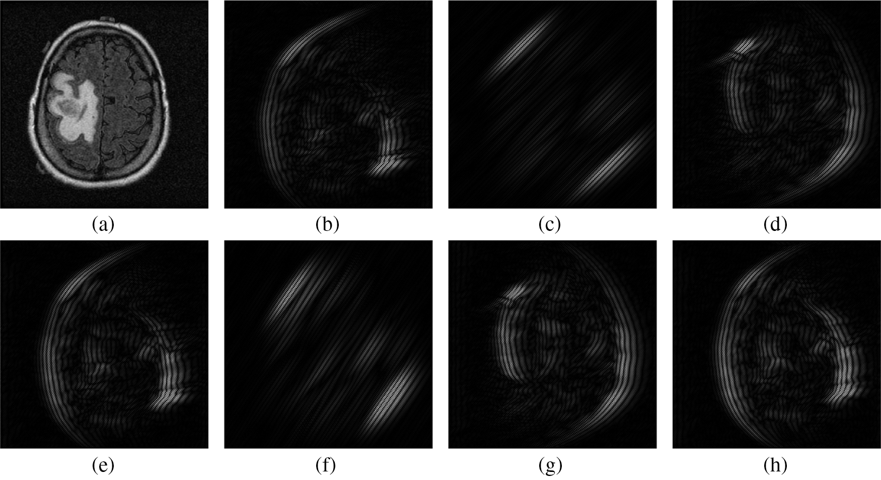
Figure 2: Textural information from Bendlet transformed sub-bands of 3-level with 8-directions. (a) Input Image (b) 1st sub-band (c) 2nd sub-band (d) 3rd sub-band (e) 4th sub-band (f) 5th sub-band (g) 6th sub-band (h) 7th sub-band
As the Bendlet is a multi-scale and multi-directional analysis, it provides a lot of textural information in the form of sub-bands. It is preferable that the prediction system is also designed on the basis of only few significant features that characterize the measurement vector. This is achieved by selecting a sub-band to be representative of the feature extraction process, while discarding redundant and less relevant sub-bands. Tab. 2 shows the number of Bendlet’s sub-bands.

To select the sub-band for feature extraction, at first the energies are computed and then statistical t-test is employed. The energy of Bendlet Sub-Band (SB) is defined in Eq. (4).
where the size of SB is X × Y and (i, j) are the co-ordinates. After extracting the energy features for a particular level and directions from the two groups (normal and abnormal or low-risk and high-risk) of MRI images, t-test is applied to identify the best sub-band that has the significant different between the two groups. The t-test [24] is defined in Eq. (5).
where nx, σx and μx are the number of samples, standard deviation and mean of classes x. A higher T value of a particular sub-band from the two classes indicates that they have more discriminating power than others. Thus the sub-band with maximum T value is chosen for feature extraction.
The BCFs can be considered as a well-known statistical measurement tool. The interdependencies of the Bendlet coefficients of the brain image textures are effectively described by BFCs. Based on the angle (θ) and displacement distance (d), a number of co-occurrence matrix can be generated. Normally, θ is quantized to 45° intervals (45°, 90°, 135° and 180°) with one or two pixels distance [25]. This matrix can be considered as a measure of 2nd order statistical interactions in the image, p(i, j|d, θ). The co-occurrence matrix (p) is defined so that each entry in the matrix, (i, j) represents the number of occurrences of the pair of intensity levels i and j which are a vector d distance aparts at an angle θ. Using a normalized co-occurrence matrix, the following feature measurements such as Energy (Eq. (6)), Correlation (Eq. (6)), Contrast (Eq. (7)) and Homogeneity (Eq. (8)) are extracted.
Energy provides a measure of intensity transition. The smooth textures are characterized by a high energy value and it indicates that the elements of p range from very high to very low.
where μ and σ2 are mean and variance of p respectively. The correlation feature is a measure of the linear dependencies in the image. A fine structure has a small correlation value because adjacent pixels are less correlated.
The contrast and Homogeneity gives the local variance and uniformity of textures in the given image respectively. Also, the contrast shows the reliable significant class defining structures. BCFs are extracted from the selected sub-band. At first, the co-occurrence matrix of selected sub-band is constructed for four angular directions (45°, 90°, 135° & 180°) and then they are normalized. The application of Eqs. (6)–(9) on the normalized matrix (p) produces four BCFs for a particular angular direction.
Histogram features are the first order statistical technique to analyze the input data. Consider the 2D input data f(x, y) which consists of a set of random variables k that represents the intensity of the pixel. The global distribution of f can be measured by generating its histogram and used as one of the important features due to its information content and simplicity. The histogram is defined in Eq. (10)
where G ∈ (0, …Ng − 1) where the number of discrete intensity levels is Ng and the number of pixels with intensity of k is denoted by nk. To extract histogram features, the positive and negative Bendlet coefficients of the selected sub-band are separated at first and then two 10-bin histograms are generated between the minimum and maximum of positive and negative coefficients respectively.
By generating the HPBC and HNBC from each MRI image and extracting features from 10-bin, it is expected that it has enough discriminating power to separate each type of brain tumour. The features used for brain image classification are based on co-occurrence and histogram of selected sub-band of Bendlet transformed brain image at different level and different directions. The actual histogram feature is computed from a set of histograms (HPBC and HNBC) obtained from the selected sub-band by t-test. The final examined feature is composed of BCFs, HPBC and HNBC. A total of 36 features are extracted from MRI brain image for the classification which includes 10 HPBC features, 10 HNBC features and 16 BCFs (4 features from each co-occurrence matrix obtained from 45°, 90°, 135° and 180°).
Fig. 3 shows the classification scheme of the BEL system. For any system used for classification, the important criterion is that the test samples be organized into well-defined groups. In this study, Group-1 consists of samples from normal and abnormal categories and Group-2 consists of samples of low-risk and high-risk categories. The grading of brain tumour is made in two stages; initial stage and final stage. The former stage uses the samples from Group-1 images and the later one uses the samples from the Group-2 images.
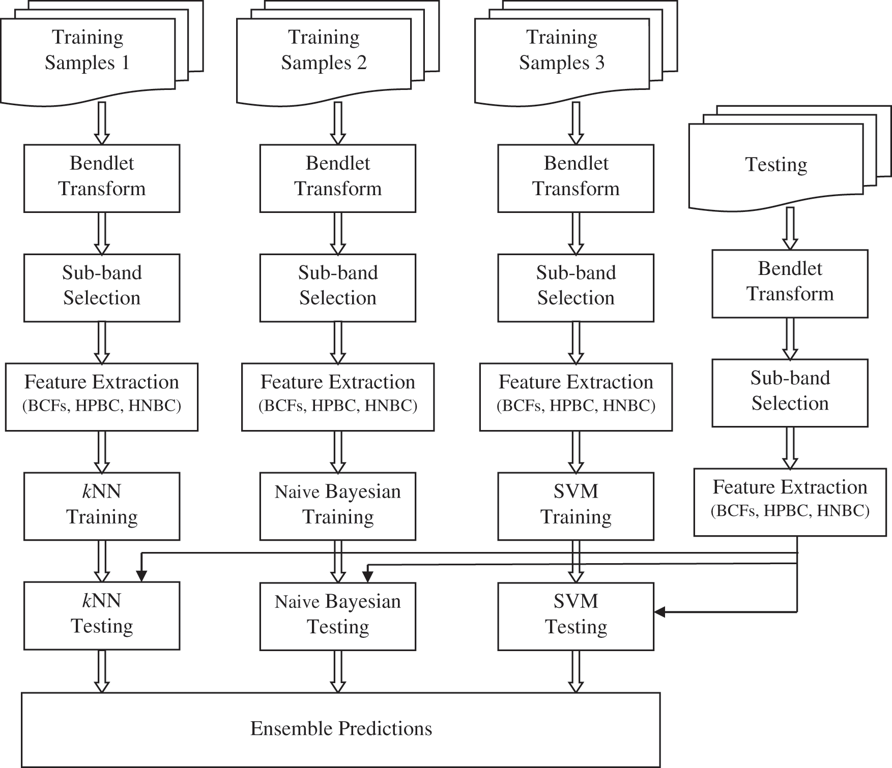
Figure 3: Classification scheme of BEL system
Three different classifiers; kNN, Naive Bayesian and SVM are used to predict the class of the MRI brain image in an ensemble manner. Brief descriptions about the classifiers are discussed below. The kNN classifier is an extension of the nearest neighbour technique which does not require any training prior to the classification. In kNN, the test data is assigned to a class that is best represented by its surrounding k-nearest neighbours. It is affected by the order in which the training samples are analyzed. The number of nearest neighbour used in this study is 1(k = 1) and Euclidean distance measure is employed to compute the distance between the testing and training features.
Perhaps most fundamental to the statistical approach of pattern recognition is Bayes’ decision theory. It considers the classification problem in probabilistic terms assuming that all relevant probability distributions of the measurements are known. It then assigns new measurements to the appropriate classes based on their class membership probabilities (posterior probabilities). It is thus natural to consider the probability distributions of MRI brain image data before proceeding to discuss the SVM classifier. According to Bayes’ decision theory there is no reason to limit the number of features or variables of the input pattern to the classifier. In practice, however, only a finite set of samples is available for the design of the classifier, and so the performance of the classifier deteriorates as the dimension of its input increases.
Mathematically, Gaussian distributions have attractive properties that make them responsible for the analysis. Naive Bayesian classifiers are optimal in terms of their expected probability of error. The probability of error of Naive Bayesian classifiers designed on data with Gaussian distributions can be derived analytically. kNN works by extending a local region around the unknown pattern x until the kth nearest neighbours-drawn out from the labeled training set are enclosed. The volume of the local region and the enclosed k nearest neighbours are random variables dependent on x. The density function is then approximated by Eq. (11).
However, the real power and usefulness of kNN lies in the fact that the density function needs not to be known or even evaluated. The classification is performed directly by approximating the posterior class probability P(Ci/x). With the unknown pattern x in the centre of the volume V(x), ki out of the captured k samples in the volume turn out to be labeled as Ci. Since the joint density function is approximated by Eq. (11) using Bayes rule P(Ci/x)p(x) = p(x, Ci) gives (Eq. (12))
with
Let us consider the equation of the hyperplane w.x + b = 0. The optimization problem that provides the best hyperplane is equivalent to minimizing
where w is normal to the plane and b is the bias. This is a quadratic programming problem and the patterns which satify the above equation are called support vectors. These samples together define the decision boundary and all other patterns can be removed. Given the optimal hyperplane, a new pattern for linear case can be predicted using
The objective function to be minimized is now
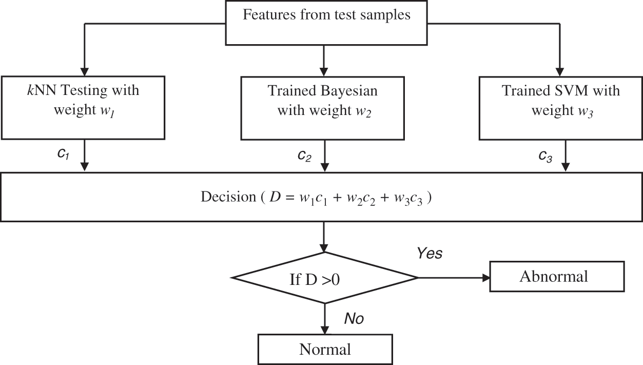
Figure 4: Ensemble prediction of the BEL system
All classifiers perform better in some situations which mainly depend on the extracted features. As each classifier has unique properties, an ensemble learning using kNN, Naive Bayesian and SVM classifiers is designed. The initial weights (wi i = 1 to 3) of these classifiers are computed based on the accuracy using different samples. Finally, the testing samples are classified by hybridizing the individual classifiers outcomes with their corresponding weights. Though all the classifiers; kNN, Naive Bayesian and SVM can able to classify three classes of samples (normal, low-risk and high-risk) at a time, this study uses the binary classification strategy and predict the brain cancer in two stages (Initial stage and Final stage). This is due the large optimization problem in multi-class classification and their complexity is more than a binary classification scenario.
For any classification system to operate as a potential classifier, the training samples should offer an accurate representation that defined each category. In this work, the training samples are obtained from the on-line freely available database; REMBRANDT database [26–28]. At first the DICOM images of size 256 × 256 are converted into bitmap format and then used for further processing. From the database, 100 normal, 50 low-risks, 50 high–risks images are selected for analyzing the BEL system. Three samples per category from REMBRANDT database images are shown in Fig. 5. The performances of the BEL system are analyzed in two stages; initial stage (normal/abnormal prediction) and final stage (low-risk/high-risk prediction). In both stages, the following performance metrics; sensitivity (Sn), specificity (Sp), and accuracy (Ac) are computed. The computation of BEL system performances are shown in Tab. 3.
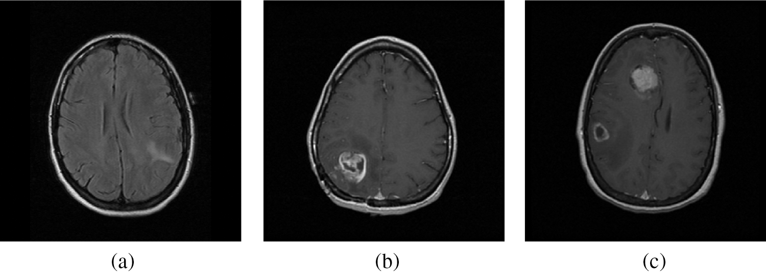
Figure 5: A sample from REMBRANDT database images. (a) Normal MRI images (b) Low-risk MRI images (c) High-risk MRI images

In practice, the performance is assessed by testing the classifier experimentally; counting the number of errors it makes and uses the results as an indicator of future accuracy. It should be noted that the samples used for training (designing the classifier) and those used for testing must be statistically independent (at least different). This is usually achieved by partitioning the available data into a training set and a test set. However, when the data is limited, one wishes to use as many samples for the design is possible. In our case, 200 images (Initial stage) and 100 images (Final stage) are used. Thus, k-fold validation is employed. Fig. 6 shows the illustration of 10-fold validation.
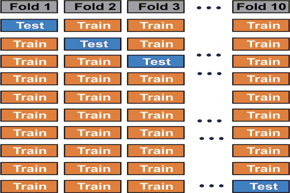
Figure 6: Illustration of 10-fold validation technique
This work uses 10-fold validation for both stages to validate the BEL system using textural features from different Bendlet levels and directions. Tabs. 4 and 5 show the performances of BEL system using 1st level and 2nd level texture descriptors.


The extraction of texture descriptors is a continuous process for 1-level starts from 2-directions to 32-directions. It can be observed from Tab. 4 that, when texture descriptors from 1-level and 8-directions used to form the feature space, the classification accuracy of BEL system is at maximum (94% at initial stage and 91% at final stage). Also it could only manage at best, 93% sensitivity and 95% specificity at initial stage and 90% sensitivity and 92% specificity at final stage. The early experiments involving 1-level descriptors are failed to produce satisfactory results and further analysis is made using 2-level descriptors for brain image analysis. It can be observed from Tab. 5 that better prediction of samples from Group-1 and Group-2 is achieved when the features are extracted from 2-level with 8-directions (96% at initial stage and 95% at final stage) which is slightly better than 1-level with 8-directions (94% at initial stage and 91% at final stage). The increase in the performance of BEL system confirms that dominant texture descriptors are extracted from the higher level of digital representation of MRI brain images. Tab. 6 shows the performances of BEL system using 3rd level texture descriptors. Tab. 7 shows the performances of BEL system using 4th level texture descriptors.


It is worth mentioning that the BEL system with 3-level & 8-directions texture descriptors provided a high classification performance of 99.5% (initial stage) and 99% (final stage), which is a nearly 3.5% (initial stage) and 4% (final stage) increase compared with the performances obtained from 2-level and it is 5.5% (initial stage) and 8% (final stage) than 1-level. The results are significant, as the basic statistical parameters; BCFS, HPBC and HNBC derived from MRI brain images, associated with the BEL system; do not require any clinical information for grading the brain tumour. The 98% and 94% accuracy (also sensitivity and specificity) for initial stage and final stage respectively, demonstrate a confidence in the 4-level with 8-directions feature’s ability to represent the MRI brain images, despite it has lower performance than 3-level descriptors. This is due to that the descriptors of 4-level affected by the redundant data at the higher levels. This offers strong evidence that further increase in the level decreases the BEL system’s performance. Also, it is observed from the performance tables, kNN is unable to perform to a similar level when compared to Naive Bayesian and SVM classifier and SVM classifier provides higher classification rate than Naive Bayesian classifier. Fig. 7 shows the maximum performance achieved by the BEL system using 3-level with 8-directions at initial stage with Receiver Operating Characteristic curves (ROCs) and Fig. 8 shows the maximum performance achieved by the BEL system using 3-level with 8-directions at final stage with ROCs.
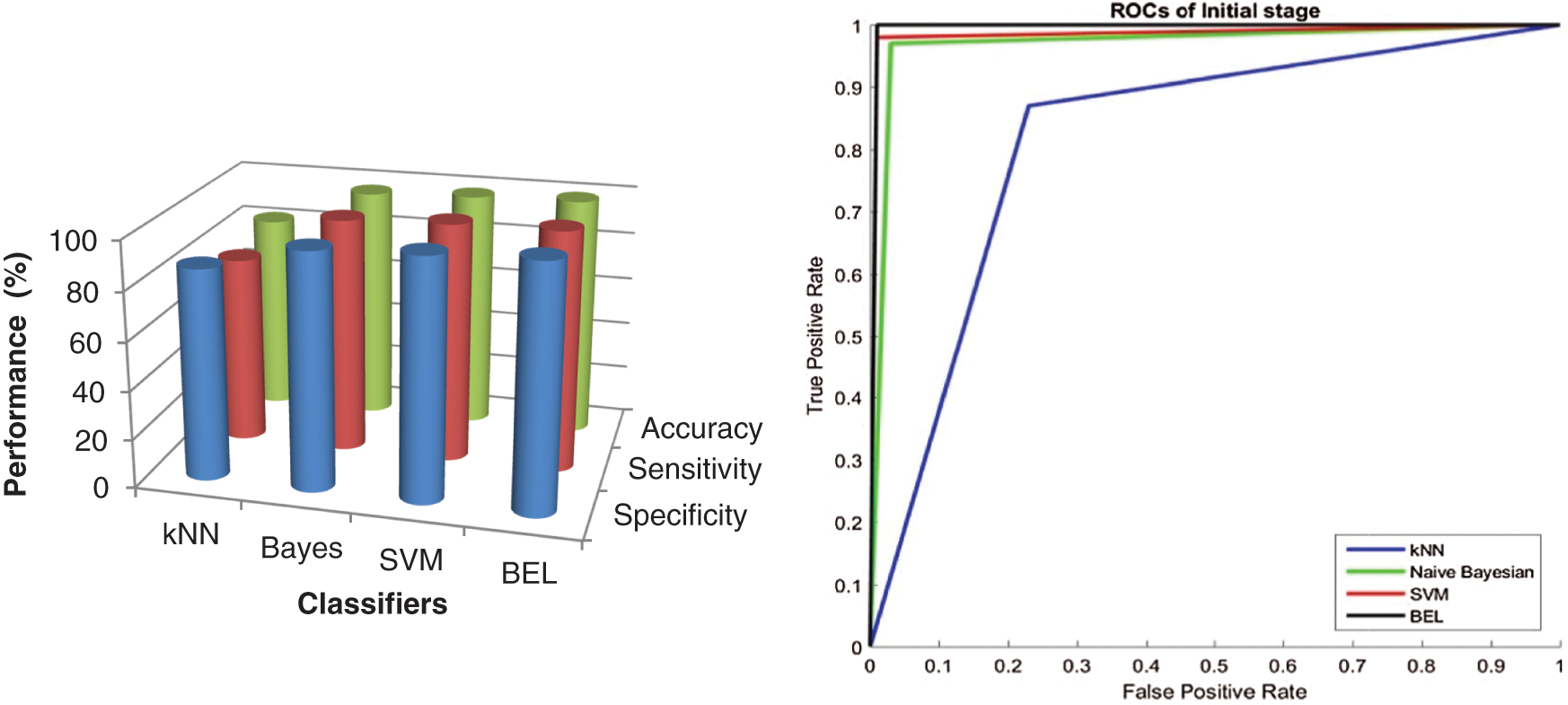
Figure 7: Performance comparison of BEL system with ROCs using 3-level (8-directions) at initial stage
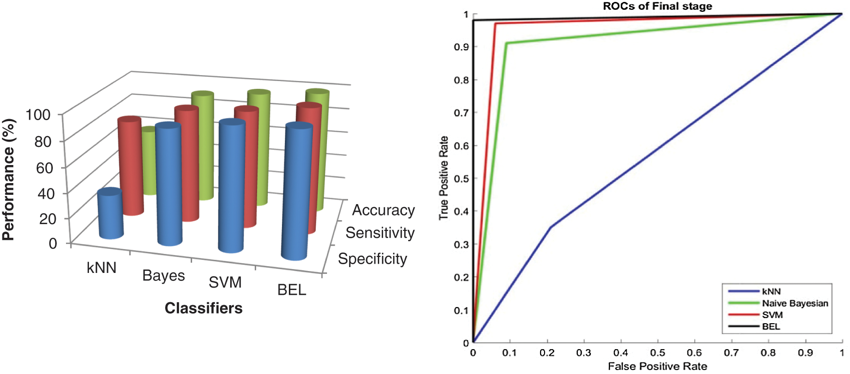
Figure 8: Performance comparison of BEL system with ROCs using 3-level (8-directions) at final stage
It can be seen from Figs. 7 and 8 that the texture descriptors used in this approach with the kNN classifier failed to produce better performance for both stages. Though Naive Bayesian and SVM classifiers managed to classify the images at best, their accuracy rates are less than 98.5%. The BEL system improves the rate of classification to overall maximum of 99.5% (initial stage) and 99% (final stage). Fig. 9 shows the comparison of BEL system with other transformation techniques.
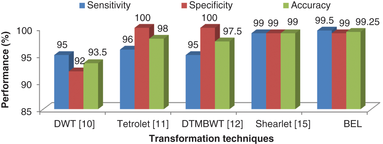
Figure 9: Comparison of BEL system with other transformation techniques
The BEL system correctly assigns the incoming samples to their corresponding category approximately 99.5% for abnormal and 99% for normal categories. The automated system would ensure that the sensitivity and specificity metric is at maximum required by the medical practitioner. The benefits such as less man power, cheap cost and an increase in reliability are achieved when using an automated system. The BEL system also eliminates the segmentation process and could lead to a practical clinical tool for grading brain tumour from MRI brain images.
The brain image analysis in this work represents a systematic approach to the classification of brain cancer using MRI brain images. The performance of any classification system is dependent upon the selected features and classifiers. Using MRI brain images, the primary objective is to extract the dominant features between the normal and abnormal images, for possible use as an automated classification system. The samples are selected from the REMBRANDT database which comprised of 200 images (100 normal, 50 low-risk and 50 high-risk). The texture descriptors such as BCFs, HPBC and HNBC extracted from the dominant sub-band of Bendlet transformed brain image with ensemble classifiers managed to produce promising results. The ideas presented in this work also offer a potential direction to improve the classification accuracy for all types of medical diagnosis.
Funding Statement: The authors received no specific funding for this study.
Conflicts of Interest: The authors declare that they have no conflicts of interest to report regarding the present study.
1. S. Mastromichalakis and S. Chountasis, “An MR image classification scheme based on Fourier moment analysis and linear support vector machine,” Journal of Information and Optimization Sciences, vol. 42, no. 1, pp. 173–191, 2021. [Google Scholar]
2. S. Mastromichalakis and S. Chountasis, “A moment based fractional Fourier transform scheme for MR image classification,” Automatic Control and Computer Sciences, vol. 55, no. 4, pp. 377–387, 2021. [Google Scholar]
3. M. Nazir, M. A. Khan, T. Saba and A. Rehman, “Brain tumor detection from MRI images using multi-level wavelets,” in IEEE Int. Conf. on Computer and Information Sciences, Sakaka, Saudi Arabia, pp. 1–5, 2019. [Google Scholar]
4. G. Latif, D. A. Iskandar, J. M. Alghazo and N. Mohammad, “Enhanced MR image classification using hybrid statistical and wavelets features,” IEEE Access, vol. 7, pp. 9634–9644, 2018. [Google Scholar]
5. A. Gudigar, U. Raghavendra, E. J. Ciaccio, N. Arunkumar, E. Abdulhay et al., “Automated categorization of multi-class brain abnormalities using decomposition techniques with MRI images: A comparative study,” IEEE Access, vol. 7, pp. 28498–28509, 2019. [Google Scholar]
6. M. Assam, H. Kanwal, U. Farooq, S. K. Shah, A. Mehmoodet et al., “An efficient classification of MRI brain images,” IEEE Access, vol. 9, pp. 33313–33322, 2021. [Google Scholar]
7. R. Mehrotra, M. A. Ansari and R. Agrawal, “Neural network and wavelet-based study on classification and analysis of brain tumor using MR images,” in IEEE Int. Conf. on Power Energy, Environment and Intelligent Control, Mumbai, India, pp. 264–269, 2019. [Google Scholar]
8. B. Deepa, M. G. Sumithra, R. M. Kumar and M. Suriya, “Weiner filter based Hough transform and wavelet feature extraction with neural network for classifying brain tumor,” in IEEE 6th Int. Conf. on Inventive Computation Technologies, Coimbatore, India, pp. 637–641, 2021. [Google Scholar]
9. P. Satapathy, S. K. Pradha and S. Hota, “An empirical performance analysis of brain image classification models using variants of neural networks,” in IEEE Int. Conf. on Applied Machine Learning, Bhubaneswar, India, pp. 87–91, 2019. [Google Scholar]
10. S. Mohankumar, “Analysis of different wavelets for brain image classification using support vector machine,” International Journal of Advances in Signal and Image Sciences, vol. 2, no. 1, pp. 1–4, 2016. [Google Scholar]
11. B. S. Babu and S. Varadarajan, “Detection of brain tumour in MRI scan images using tetrolet transform and SVM classifier,” Indian Journal of Science and Technology, vol. 10, no. 19, pp. 1–10, 2017. [Google Scholar]
12. R. R. Ayalapogu, S. Pabboju and R. R. Ramisetty, “Analysis of dual tree M-band wavelet transform based features for brain image classification,” Magnetic ResonanceiIn Medicine, vol. 80, no. 6, pp. 2393–2401, 2018. [Google Scholar]
13. L. Fang, H. Zhang, J. Zhou and X. Wang, “Image classification with an RGB-channel nonsubsampled contourlet transform and a convolutional neural network,” Neurocomputing, vol. 396, pp. 266–277, 2020. [Google Scholar]
14. R. Zia, P. Akhtar, A. Aziz and M. A. Shah, “Non sub-sampled contourlet transform based feature extraction technique for differentiating glioma grades using MRI images,” Australasian Joint Conf. on Artificial Intelligence, Melbourne, VIC, Australia, pp. 289–300, 2017. [Google Scholar]
15. R. Muthaiyan, and M. Malleswaran, “An automated brain image analysis system for brain cancer using shearlets,” Computer Systems Science and Engineering, vol. 40, no. 1, pp. 299312, 2022. [Google Scholar]
16. K. Beyer, J. Goldstein, R. Ramakrishnan and U. Shaft, “When is “nearest neighbor” meaningful?,” in Int. Conf. on Database Theory, Jerusalem, Israel, pp. 217–235, 1999. [Google Scholar]
17. I. Rish, “An empirical study of the naive Bayes classifier,” International Workshop on Empirical Methods in Artificial Intelligence, vol. 3, no. 22, pp. 41–46, 2001. [Google Scholar]
18. C. Cortes and V. Vapnik, “Support-vector networks,” Machine Learning, vol. 20, no. 3, pp. 273–297, 1995. [Google Scholar]
19. S. Mallat, A Wavelet Tour of Signal Processing: The Sparse Way. Academic Press, Elsevier, United States of America, 2008. [Google Scholar]
20. D. Donoho and E. Candes, “Continuous curvelet transform: II. Discretization and frames,” Applied and Computational Harmonic Analysis, vol. 19, no. 2, pp. 198–222, 2005. [Google Scholar]
21. M. N. Do and M. Vetterli, “The contourlet transform: An efficient directional multiresolution image representation,” IEEE Transactions on Image Processing, vol. 14, no. 12, pp. 2091–2106, 2005. [Google Scholar]
22. W. Q. Lim, “The discrete shearlet transform: A new directional transform and compactly supported shearlet frames,” IEEE Transactions on Image Processing, vol. 19, no. 5, pp. 1166–1180, 2010. [Google Scholar]
23. C. Lessig, P. Petersen and M. Schäfer, “Bendlets: A second-order shearlet transform with bent elements,” Applied and Computational Harmonic Analysis, vol. 46, No. no. 2, pp. 384–399, 2019. [Google Scholar]
24. R. Thamizhamuthu and D. Manjula, “Skin melanoma classification system using deep learning,” Computers, Materials & Continua, vol. 68, no. 1, pp. 1147–1160, 2021. [Google Scholar]
25. R. M. Haralick, K. Shanmugam and I. H. Dinstein, “Textural features for image classification,” IEEE Transactions on Systems, Man and Cybernetics, vol. 6, pp. 610–621, 1973. [Google Scholar]
26. K. Clark, B. Vendt, K. Smith, J. Freymann, J. Kirby et al., “The cancer imaging archive (TCIAMaintaining and operating a public information repository,” Journal of Digital Imaging, vol. 26, no. 6, pp. 1045–1057, 2013. [Google Scholar]
27. Brain MRI images: https://wiki.cancerimagingarchive.net/display/Public/REMBRANDT. [Google Scholar]
28. L. Scarpace, A. E. Flanders, R. Jain, T. Mikkelsen and D. W. Andrews, “Data from REMBRANDT,” The Cancer Imaging Archive, http://doi.org/10.7937/K9/TCIA.2015.588OZUZB, 2015. [Google Scholar]
 | This work is licensed under a Creative Commons Attribution 4.0 International License, which permits unrestricted use, distribution, and reproduction in any medium, provided the original work is properly cited. |