DOI:10.32604/iasc.2022.023835
| Intelligent Automation & Soft Computing DOI:10.32604/iasc.2022.023835 | |
| Article |
Artificial Intelligence Based PID Controller for an Eddy Current Dynamometer
1Ceyhan Engineering Faculty, Mechanical Engineering Department, Çukurova University, Adana, Turkey
2Faculty of Engineering, Mechanical Engineering Department, Çukurova University, Adana, Turkey
*Corresponding Author: İhsan Uluocak. Email: iuluocak@cu.edu.tr
Received: 23 September 2021; Accepted: 04 November 2021
Abstract: This paper presents a design and real-time application of an efficient Artificial Intelligence (AI) method assembled with PID controller of an eddy current dynamometer (ECD) for robustness due to highly nonlinear system by reason of some magnetism phenomena such as skin effect and dissipated heat of eddy currents. PID Control which is known as the most popular conventional control method in industry is inadequate for such nonlinear systems. On the other hand, Adaptive Neural Fuzzy Interference System (ANFIS), Single Hidden Layer Neural Network (SHLNN), General Regression Neural Network (GRNN), and Radial Basis Neural Network (RBNN) are examples used as artificial intelligence-based techniques that can increase the performance of conventional control systems in particular. The proposed control system proves changeable Kp (Proportional gain), Ki, (Integral gain) and Kd (Derivative gain) parameters in real-time to adapt and presents a good capacity to adapt nonlinearities and bring robustness using 4 different versatile soft computing methods of ANFIS, SHLNN, GRNN, and RBNN. The testing dataset is extracted from experimental studies and its robustness has also been verified with different Artificial Intelligence (AI) methods. The presented technique is observed to have a good performance in terms of response time (t) and accuracy of desired speed value (V) under different parameters such as non-linear dynamics (V, T) of the system elements and the varying load effects.
Keywords: Eddy current; dynamometer; PID; ANFIS; SHLNN; GRNN; RBNN
The automotive companies have been using the Eddy Current Dynamometers (ECD) as an auxiliary braking system, especially for engine testing and analyzing operations. The operational principle behind this brake system is based on the electromagnetic induction theory called “Eddy Current” phenomenon. The Eddy Currents are generated at the moment when a conductive material moves inside a magnetic field. These currents generated on the conductive material as a result of the magnetic field interaction are formed as circles due to the inexact way to move. The circles unite and create eddies on the moving material. The Eddy Currents emerge a magnetic field against the magnetic field of coils that concludes a force opposes motion. The Eddy Currents are one of the most undesirable things for many applications such as AC motors. The fundamentals of Eddy Current dynamometers are discovered by Faraday i.e., the Faraday induction law [1]. Eddy current dynamometer uses this braking effect to achieve contactless and zero carbon footprint braking system.
The most severe drawback of the eddy current dynamometer is the huge amount of excitation current that may lead to serious safety issues. In addition, there may be other problems including skin effect, demagnetization effect, excessive magnetism [1–3]. The most important disadvantage of Eddy Current Dynamometer is that the braking performance varies unexpectedly divergent rotor speeds especially after nearly 1000 rpm (revolutions per minute) [2–4]. Likewise, the temperature of the rotor also affects the braking performance [5]. In addition, internal combustion engines have nonlinear torque output behavior with respect to engine speed. When these problems combine, robust controlling of this system with conventional linear control systems becomes nearly impossible. To overcome this problem, there are some solutions proposed.
In literature, many studies focus on the control strategies of Eddy Current Brakes. Tan et al. [6] introduced a linear Eddy Current Damper that has 400 mm length. He also estimates parameters and used by a PD controller. On the other hand, Simeu et al. [4] give a relationship for dragging force at low speeds. After that, they offer nonlinear modeling for Eddy Current Brakes. Finally, they proposed a two-observer nonlinear compensator to regulate the speed at a reference value. Gosline et al. [1] proposed a time-domain passivity control algorithm for Eddy Current Brakes used on the haptic braking system. Anwar [5] developed an ECB (Eddy Current Brake) system for improving the ABS (Anti-Lock Braking System) performance of the car. He used former knowledge of ECB brake performance and parameter values and added ECB for every wheel of the car with a generator that supplies energy to coils. He proposed taking the wheel speed, pressure, ECB voltage, generator output and drive each wheel motion with a sliding mode control (SMC) algorithm. Roozbehani et al. [7] proposed a technique that combines Fuzzy and PI control approaches. Yang et al. [8] proposed model-based control for Eddy Current Brakes. Xu et al. [9] suggests indirect adaptive Fuzzy H∞ control for novel Eddy Current Retarder.
Many researchers have examined Artificial Intelligence-based PID control. Jin et al. [10] used Fuzzy-based PID control to overcome nonlinearities and low output accuracy of the transplanting manipulator. Moreover, Moura et al. [11] designed a structure ANN (Artificial Neural Network) for online PID parameters tuning on mining system. Garima et al. [12] decreased harmonic distortion by using ANFIS supervised PID control system. RBNN coupled with PID was demonstrated to be effective in the paper of Kejian et al. [13] for ultra-high-voltage (UHV) gas-insulated switchgear (GIS), Zhou et al. [14] for Dissolved oxygen control in circulating aquaculture, Ma et al. [15] for the control of air gap between rail and electromagnet in Maglev System, Hoang-Dung et al. [16] for controlling the position of the carriage, and Nie et al. [17] for longitudinal speed control of autonomous vehicle. Also, Feroz Mirza et al. [18] carried out GRNN reinforced PID algorithm for another nonlinear system of PV energy collectors. In this study, it is observed that there is a need for Artificial Intelligence-based control methods on Eddy Current Dynamometers. Therefore, Single Hidden Layer NN-tuned PID, ANFIS-tuned PID, GRNN tuned PID and RBNN tuned PID controllers are designed for an Eddy Current internal combustion test bed and a comparative study in real-time is carried out practically. The rest of the paper is organized as follows. Eddy Current testbed is briefly explained in Material and Methods section. Results are shown and discussed in Result and Discussion section. The final section concludes results achieved.
Experiments were conducted in the Eddy Current Dynamometer rig located in the laboratories of Automotive Engineering Department at Cukurova University. The mechanical system consists of several parts that are illustrated in Fig. 1. A 3.1-liter internal combustion (IC) engine is granted by Başak Tractor company and used for the generation of the motion. It produces 71 HP maximum power at 2500 rpm. The maximum torque of the Telma Eddy Current Brake is used to load the IC motor with 1300 Nm at an angular speed of 1000 rpm. The Telma Eddy Current Brake is granted by Temsa company.
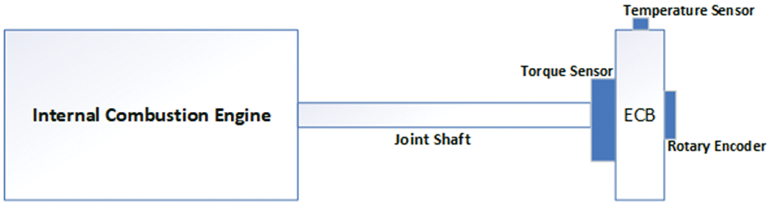
Figure 1: Schematic of eddy current testbed
The Eddy Current Dynamometer assemble is joint at a contact point. The contact point unites the rotor and stator which carries the load cell and the coils that conduct the magnetic field. The rotor is mounted to a connecting shaft, the IC engine, Eddy Current Brake and encoder as visualized in Fig. 1.
The Eddy Current Brake is used to generate the stopping effect on testing system (IC engine, Electric motor etc.) for controlling the speed of the torque shaft. The Eddy Current Dynamometer is used to simulate operating conditions of motor applications, motor control research and production, repair tests. In this study, Telma brand retarder is used that has a linear braking force ranging between 0 and 1000 rpm values. At higher speeds, braking torque acts nonlinearly as the nature of the magnetic field results in skin effect, demagnetizing effects, and less time for inducing eddy currents. The details of the experimental setup are illustrated in Fig. 2.
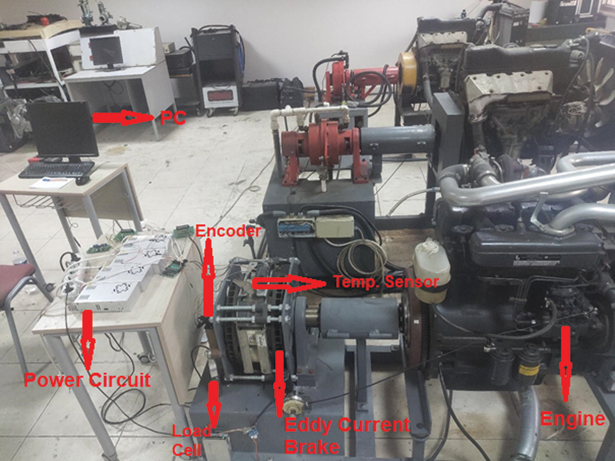
Figure 2: Photo of the eddy current dynamometer
The power supply of Eddy Current Brake has a capacity of PWM output of 80 A with 256 resolutions. This means the control signal defined a specific value that is between 0 and 256. A PC with Intel i3 microprocessor (3.9 GHz) and 16 GB RAM is utilized to carry out the calculations required for the control signal and artificial intelligence calculations in MATLAB/Simulink environment. The calculated control signal is sent by the Microcontroller Unit (MCU) card to the eddy current driver that can run 100 A, 2400 W devices. The MCU card is selected as Arduino Mega 2560 due to its versality and MATLAB/Simulink linking ability. The speed of the shaft is measured with a line drive magnetic encoder with a resolution of 360 (pulse/rotation). Meanwhile, a load cell and contactless infrared temperature sensor are also used in the sensory system. Fig. 3 depicts the electronic layout of the control system. The Arduino Mega 2560 connects the sensors, eddy current dynamometer coils to MATLAB/Simulink that maintains the connections with an add-on called “ArduinoIO”. Arduino Mega 2560 can perceive input and send output signals with 54 Digital Input (15 PWM) for and 16 analog input pins. The Eddy current brake driver have 2 inputs and 1 output which is a 24 VDC PWM current left for coils. The first input is 24 VDC feed power input and the other is 0–5 V PWM signal that controls the power delivered to the coils.
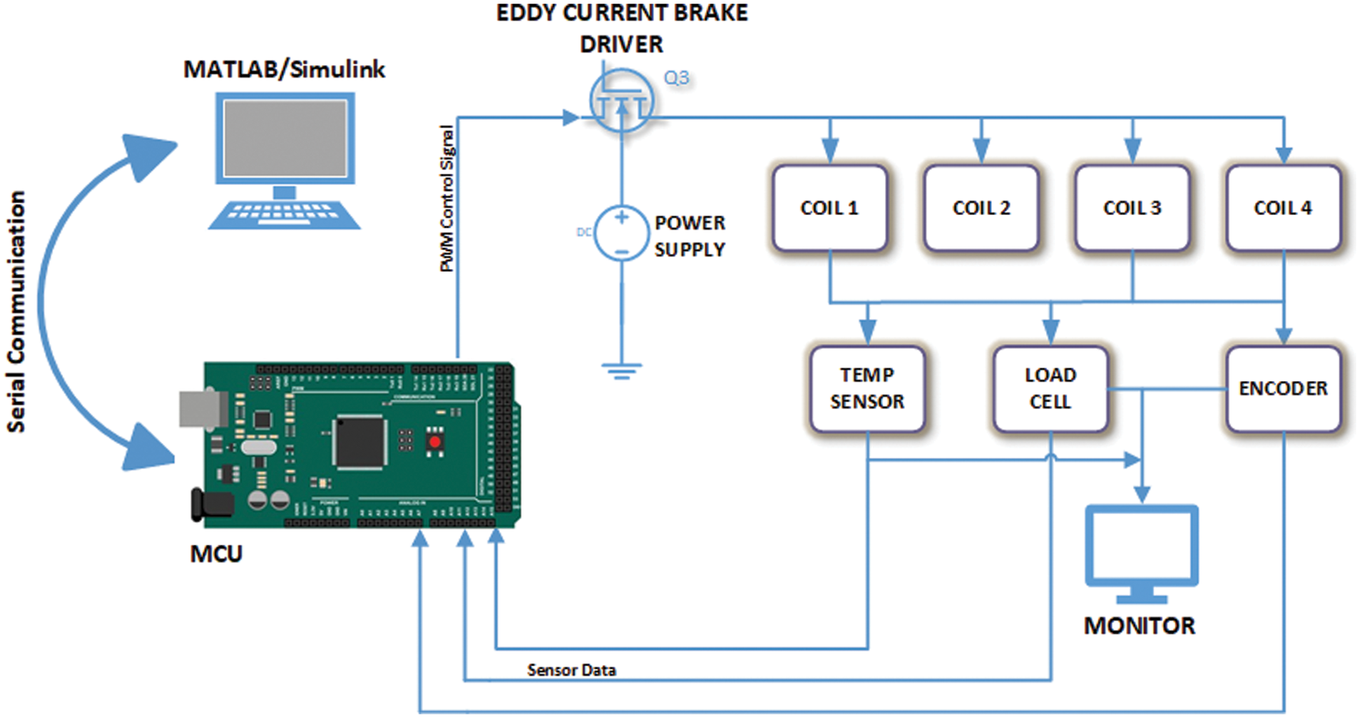
Figure 3: The electronical control schema
In order to find out the capabilities of the magnetic retarder, system identification and parameter estimation tasks have to be done. The parameters of shaft speed and rotor temperature have a huge effect on the braking performance of the retarder. Hence, the system behaviors can be predicted with respect to speed and temperature changes.
The Eddy Current Dynamometers are naturally nonlinear since their braking torque changes unpredictably with rotor speed and rotor temperature. It is well known torque produced by eddy current brake is related to conductivity of the rotor as seen on Eq. (1):
where σ is conductivity of rotor and Tb is produced torque. Heating occurs during the braking process leads to increase in the rotor temperature. Hence, the conductivity of metal rotor decreases irregularly at the same time as temperature increases. In this regard, hotter rotor causes less torque produced based on a nonlinear manner. To determine the nonlinear performance of the system, the step response of the eddy current dynamometer speed against PWM load has been tested for 1800–3000 rpm range with a resolution of nearly 100 rpm. In addition to speed, the temperature of the Eddy Current Dynamometer rotor is measured at 4 different values between 25 and 100°C for each speed measurement. The results of each step response experiment yield graphs which can lead us to linearize the system and determine Kp, Ki, and Kd values using the highest slope of the graph (N) and delay time (L) of the eddy current dynamometer response according to Process-Reaction Curve (PRC) method as pictured on Fig. 4. Therefore, the nonlinear eddy current braking system is linearized, and a robust hybrid control system is completed successfully. Entire system’s block diagram is illustrated in Fig. 5.
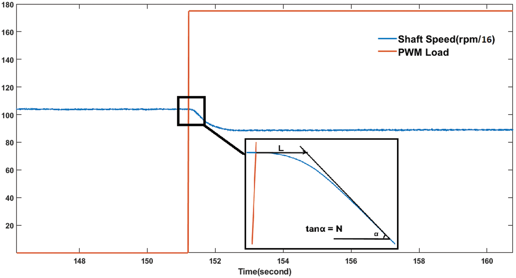
Figure 4: Sample of process reaction curve calculation
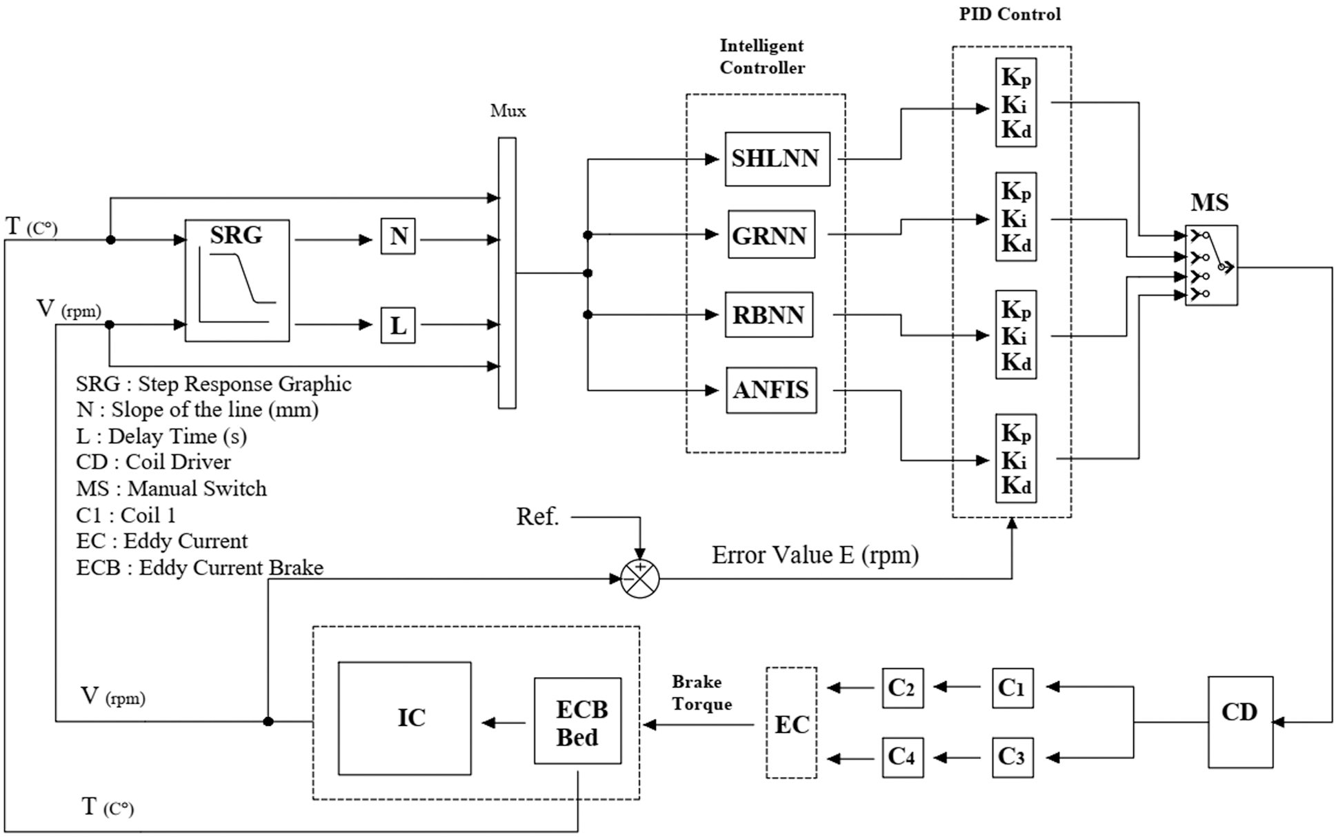
Figure 5: Block diagram of adaptive PID control
PID is a control method that combines proportional, integral, and derivative of the input error, helping the unit to automatically compensate for changes as seen in Fig. 6. The mathematical expression is given by;
The main advantage of PID control is the wide application areas including mechanical systems, hence in most engineering applications as commonly accepted, PID control is proved to be the most suitable control method [14–16]. In the industrial field, process control systems basic and modified PID control has shown to have satisfactory control performance [11,12,15]. Although there are many given situations proved, they are not really suitable for nonlinear systems.
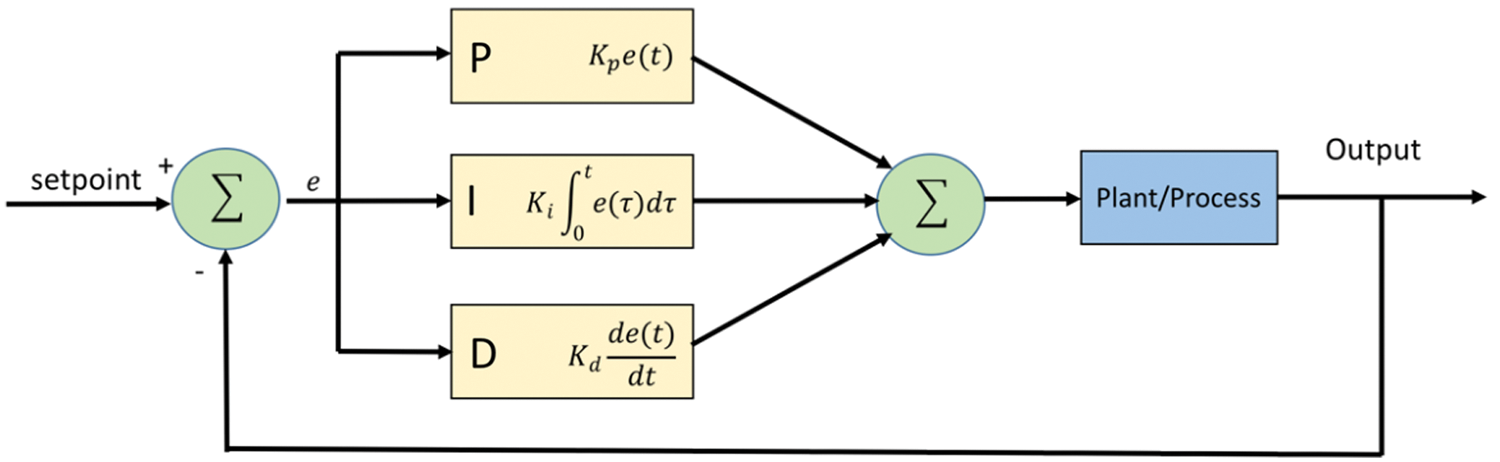
Figure 6: PID structure
Biological nervous systems and mathematical systems’ learning theories inspired the Artificial Neural Network (ANN) systems. The learning procedure of ANN is achieved by various mesh of processing nodes and connections. Neural Networks are simply defined as massively parallel interconnected networks of simple (usually adaptive) elements. Their hierarchical organizations are intended to interact with objects of the real world in the same way as biological nervous systems do [19,20].
In this study, Neural Fitting (nftool) Toolbox was used while training SHLNN (single hidden layer neural network) in Matlab/Simulink. Multilayer networks are forward linked and consist of three different layers called the input layer, hidden layers, and output layer. The supervised learning technique is one of the methods used by the multi-layer networks as in our case. The learning rule of the multilayer network is a generalized version of the Delta learning rule, which consists of two stages. In the first stage, forward calculations are made, then, in the second stage, backward calculations are made. So, training algorithm’s name is Levenberg–Marquardt back propagation (trainlm). Each neuron consistently contains a sigmoid activation function in its structure. The key point is that the function must be derivable since the derivative of the function used here will be taken in the backward calculation. The two-layer feed-forward network consists of sigmoid hidden neurons and linear output neurons as seen on Fig. 7.

Figure 7: SHLNN structure
There are various types of NNs for use of different purposes in literature. One of them is Generalized regression neural network (GRNN). A GRNN is suitably designed for function approximation purposes. [18]. The GRNN has faster learning and higher convergence to the optimum recession surface according to the number of samples, GRNN’s handling noises in the inputs, and requirement only a smaller number of datasets can be listed as its advantages [18]. The structure of GRNN is shown in Fig. 8.
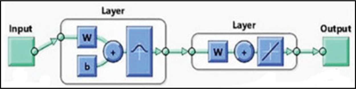
Figure 8: GRNN structure
Radial basis neural networks (RBNN) have advantages of easy design, good generalization, strong tolerance to input noise, and online learning ability [13–17,21,22]. The properties of RBNN networks make it very suitable to design of flexible control systems. Radial basis neural networks are specialized for system control applications and approximation purposes. Details of the structure can be seen in Fig. 9.
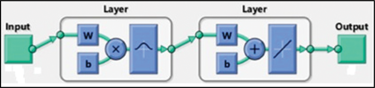
Figure 9: RBNN structure
ANFIS word comes from Adaptive Neuro-Fuzzy Interference System. ANFIS builds a Fuzzy Interference System (FIS) using a selected input/output data block. FIS membership function parameters are adjusted (tuned) with help of the back-propagation algorithm or hybrid version of the least square method and back-propagation algorithm. Hence, the tuning process lets the Fuzzy systems learn from the input/output data block.
FIS is one of the most popular artificial intelligence methods. It is solely based on human expert experience to make a decision. Therefore, the success of FIS decisions is related to either the accuracy of experts or converting these experiences from real-world to fuzzy logic interface [12,23]. Unlike FIS, ANFIS doesn’t need expert experience. Instead of it, ANN technique uses input/output data set as shown in Fig. 10.
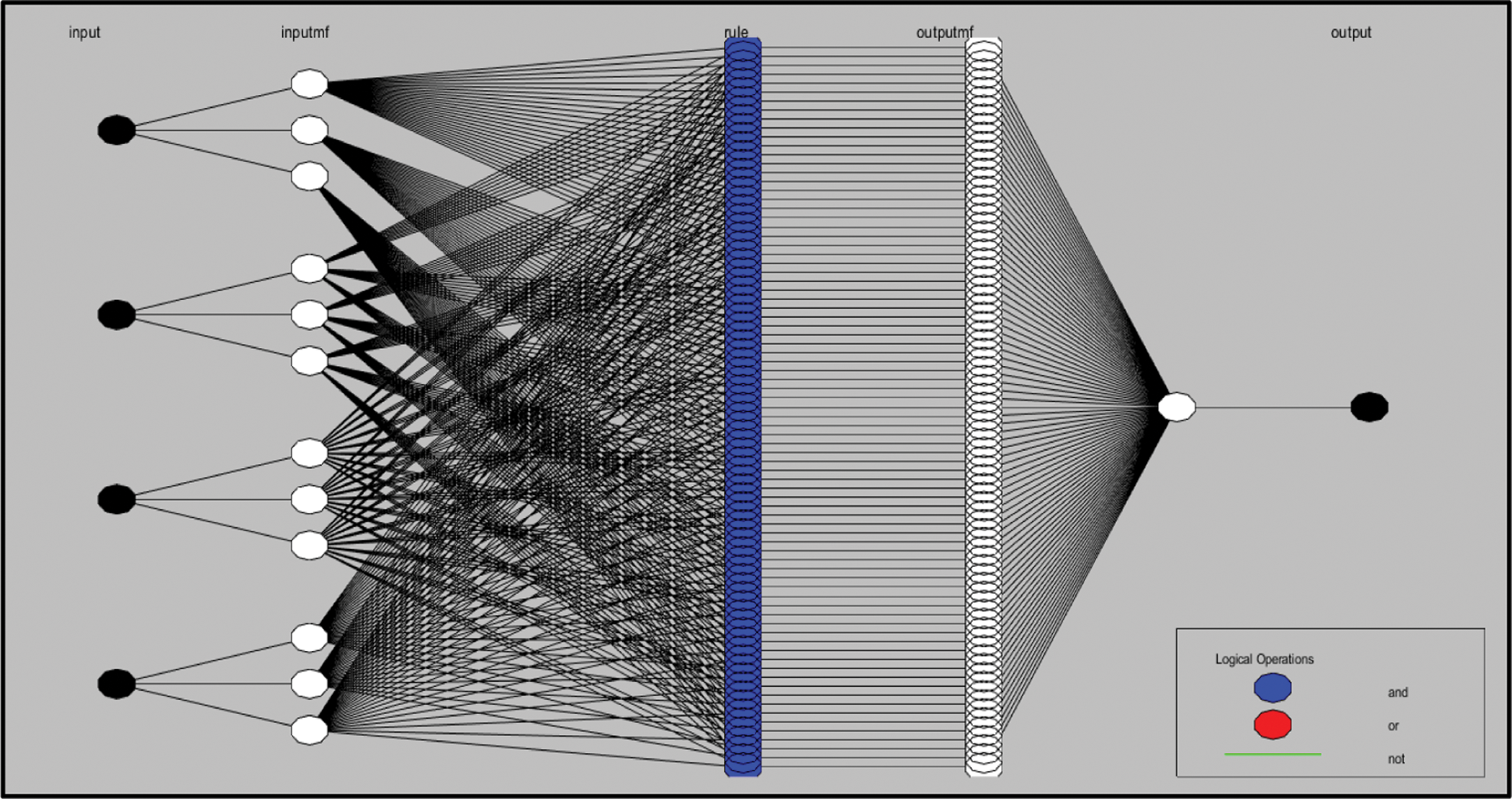
Figure 10: Sample of an ANFIS structure
The main advantages of ANFIS are [24];
• ANFIS can design nonlinear functions of arbitrary complexity using data blocks.
• ANFIS can be coupled with conventional control techniques.
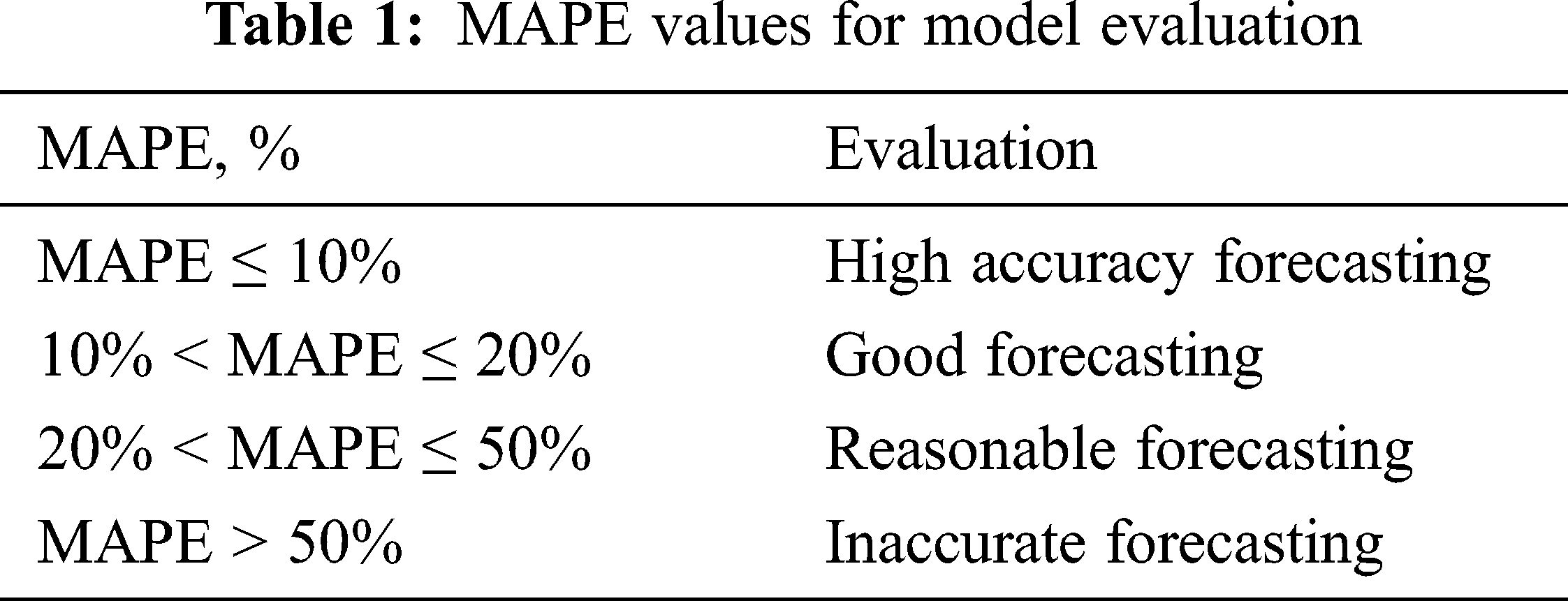
In this paper, ANFIS and PID conventional control techniques are augmented. The convergence of results is performed by the Mean Average Percent Error (MAPE) given by Eq. (3):
Here, T and O are target and output values, respectively. Mean absolute error, root-mean-square error, and MAPE are generally used to measure the accuracy of forecasts. The smaller the values of the aforementioned performance parameters, the better the forecast accuracy. MAPE criterion is more decisive among others since it is stated in easy equivalent percentage terms. Tab. 1 demonstrates typical MAPE values for model assessment [19].
Figs. 7–10 show various learning structure of used AI methods. The built ANN structures have 4 inputs. These are rotor temperature (T), speed of the dynamometer connecting shaft (V), and N, L parameters. The N and L parameters are adopted from step response graphs. Three ANN and ANFIS with one output is built for Kp, Kd, and Ki values separately.
A SHLNN, an ANFIS, a GRNN, and a RBNN structures are constructed based on system dynamics and previous studies. The gathered experiment results prove that the training algorithm of backpropagation is substantially satisfactory for predicting Kp, Kd, and Ki for various shaft speeds (V), Eddy Current Brake rotor temperature (T), N and L values. 69 datasets were obtained and 8 of them were selected as the testing data for each AI structures to avoid calculation error.
The SHLNN, ANFIS, GRNN, and RBNN predictions for Eddy Current Dynamometer achieved quite successful results against test data that are represented in Fig. 11. For the Kp value, the amount of training hidden neuron number of SHLNN is 10, and the training algorithm is Levenberg–Marquardt. 61 rows of input data are presented randomly while 70% (42) of input data is used for training job, 15% (9) is used as validation job, lastly, 15% (9) is used as testing. 8 selected data left are used for testing of built SHLNN structure.
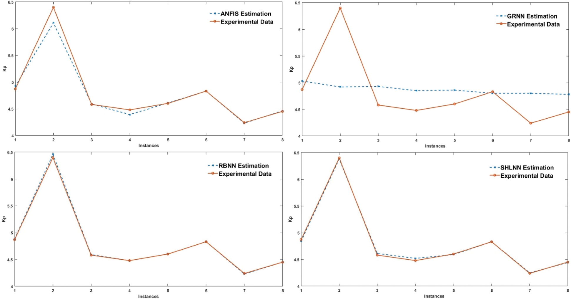
Figure 11: Comparison of testing data with estimated values of SHLNN, ANFIS, GRNN, and RBNN for Kp
Test values for Kp have an interval of 102.45 and 67.78. MAPE values are found as 0.43 for all steps after 19 epochs. Also, designed ANFIS for Kp has an amount of training membership function of 3 for each input resulting and 12 input gaussmf membership functions. 61 rows of all data for training and 8 rows of all data for were used testing. MAPE value is found 1.09 after 4 epochs. The spread value has a critical role for the GRNN and RBNN algorithms. 1, 5, 25, 50, 75, 100, 150, 250, 750, 1750, 3000 spread values were tried to optimize the optimum spread number for Kp, Kd, and Ki with 61 training data and 8 test data. Finding the correct spread value is accomplished using trial and error method. Mean squared error goal of RBNN is always picked as 0. Optimum MAPE results of RBNN for Kp were found as 0.18 at 250 spreads. On the other hand, GRNN has a relatively lower performance with best MAPE value of 8.66 at 50 spreads even it is under the limits of successful estimation according to Tab. 1.
The Ki value for test data varies between 8.84 and 13.2. The training parameters for the Ki value of the SHLNN were determined using 61 lines of input data, the number of hidden neurons was 10 and the training algorithm was Levenberg–Marquardt. Of the input data 61, 70% (42) is used for training work, 15% (9) as validation work, and finally 15% (9) as testing. 8 different data are spared for testing of built SHLNN structure. The best MAPE value was observed as 1.70 in the 9th epoch. Also, the number of nodes of the ANFIS system, which is established with 81 fuzzy rules and 12 input gaussmf membership functions for each input parameter, is 193. MAPE values were 0.93 after 40 epochs. Moreover, Ideal GRNN and RBNN spread values are found as 25 and 100, resulting in MAPE of 3.99 and 0.01, respectively. The details of the performance comparison of testing data are depicted in Fig. 12.
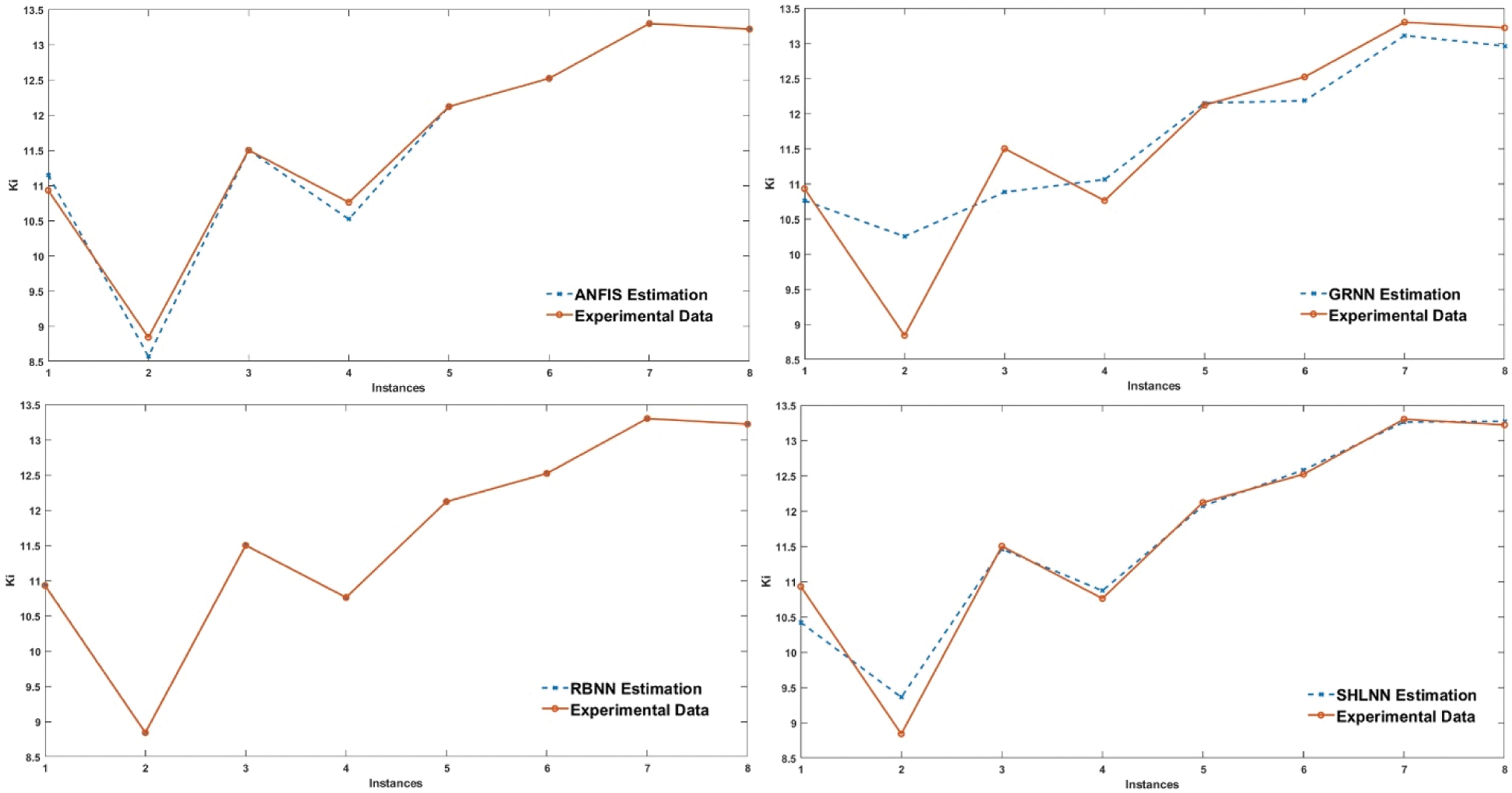
Figure 12: Comparison of testing data with estimated values of SHLNN, ANFIS, GRNN, and RBNN for Ki
Fig. 13 illustrates achieved results for Kd. The SHLNN has hidden neuron number of 10 and training algorithm of Levenberg–Marquardt, presented 61 rows of input data while 70% (42) of input data is used for training job, 15% (9) is used as validation job, lastly, 15% (9) is used as testing. Testing of built SHLNN structure is done with 8 selected data from test set. MAPE value is found as 3.04 after 85 epochs. Secondly, 3 training membership functions for each input resulting in 81 Fuzzy rules and 12 input gaussmf membership functions for 4 each input with 193 nodes are included in ANFIS network. MAPE values are calculated as 0.93 after 40 epochs. The most accurate result using GRNN is the MAPE values for Kd, 3.43 at 18 spreads, and 0.13 using RBNN at 50 spreads. ANFIS, GRNN, and RBNN structure are built using 61 sets as training data and 8 sets as testing data.
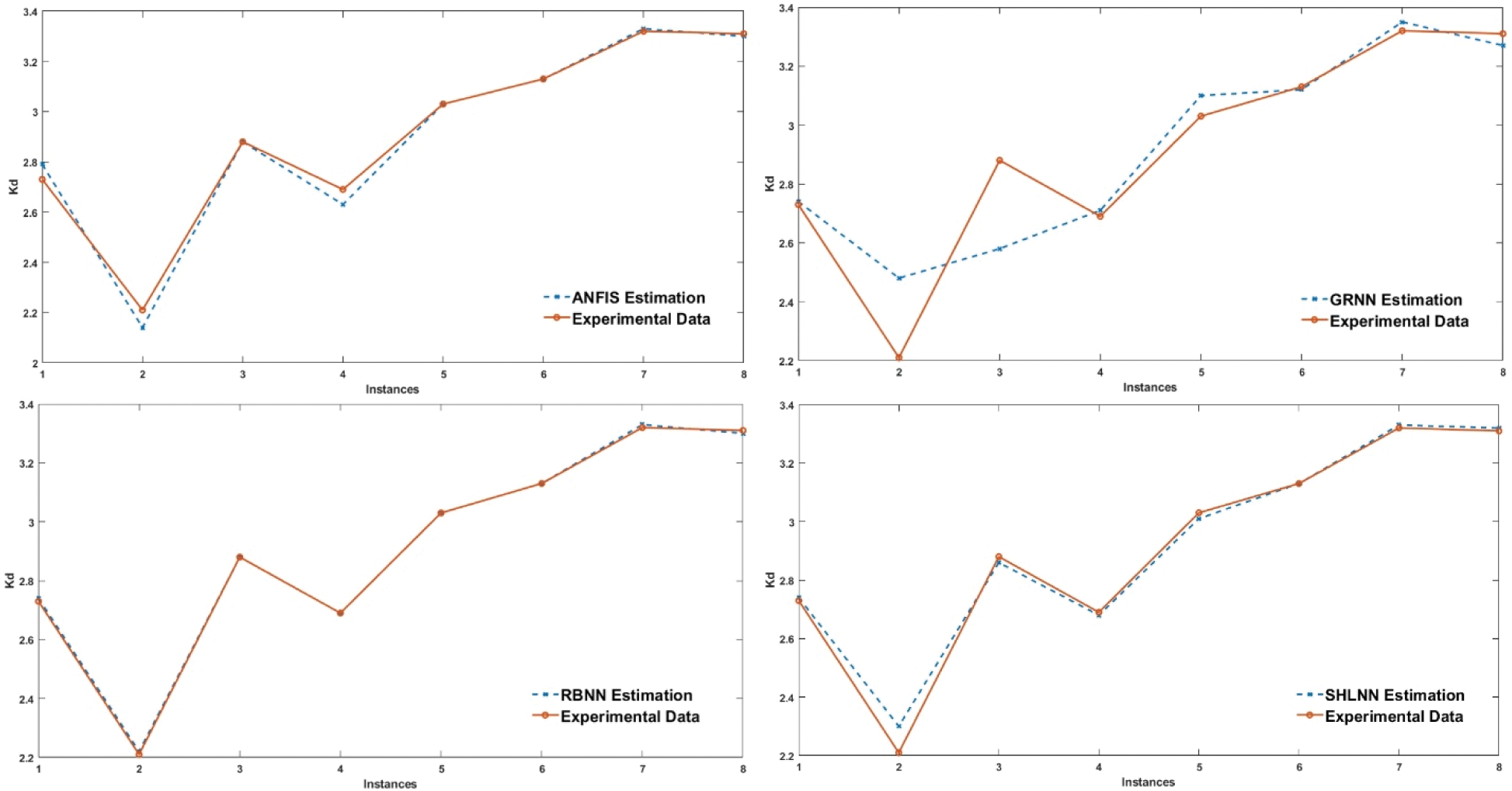
Figure 13: Comparison of testing data with estimated values of SHLNN, ANFIS, GRNN, and RBNN for Kd
Eventually, the results show that SHLNN, ANFIS, GRNN, and RBNN training procedures have been predicted successfully for the Kp, Ki and Kd values. A comprehensive study is done and the results are discussed in detail in Tab. 2 that indicates MAPE values of training by SHLNN, ANFIS, GRNN, and RBNN. Gathered results are implemented on a MATLAB/Simulink environment to achieve real-time shaft speed control of an ECB. The Simulink diagram is built regarding to evaluate the control application. The temperature sensor, encoder and analog signal blocks read information from infrared temperature sensor, encoder and loadcell. The torque value measured by load cell is logged but not included to control application. The shaft speed, and rotor temperature information is sent to Artificial Intelligence subsystem which is consist of the Simulink blocks for neural network and fuzzy logic simulation and calculations. Eventually, Variable PID controller and reference speed block is generated. Kp, Ki and Kd parameters are provided from AI subsystem and error is calculated by difference of the shaft speed and reference value as pictured in Fig. 14.
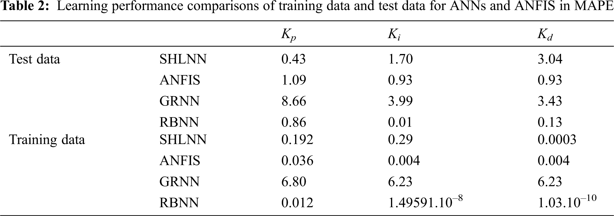
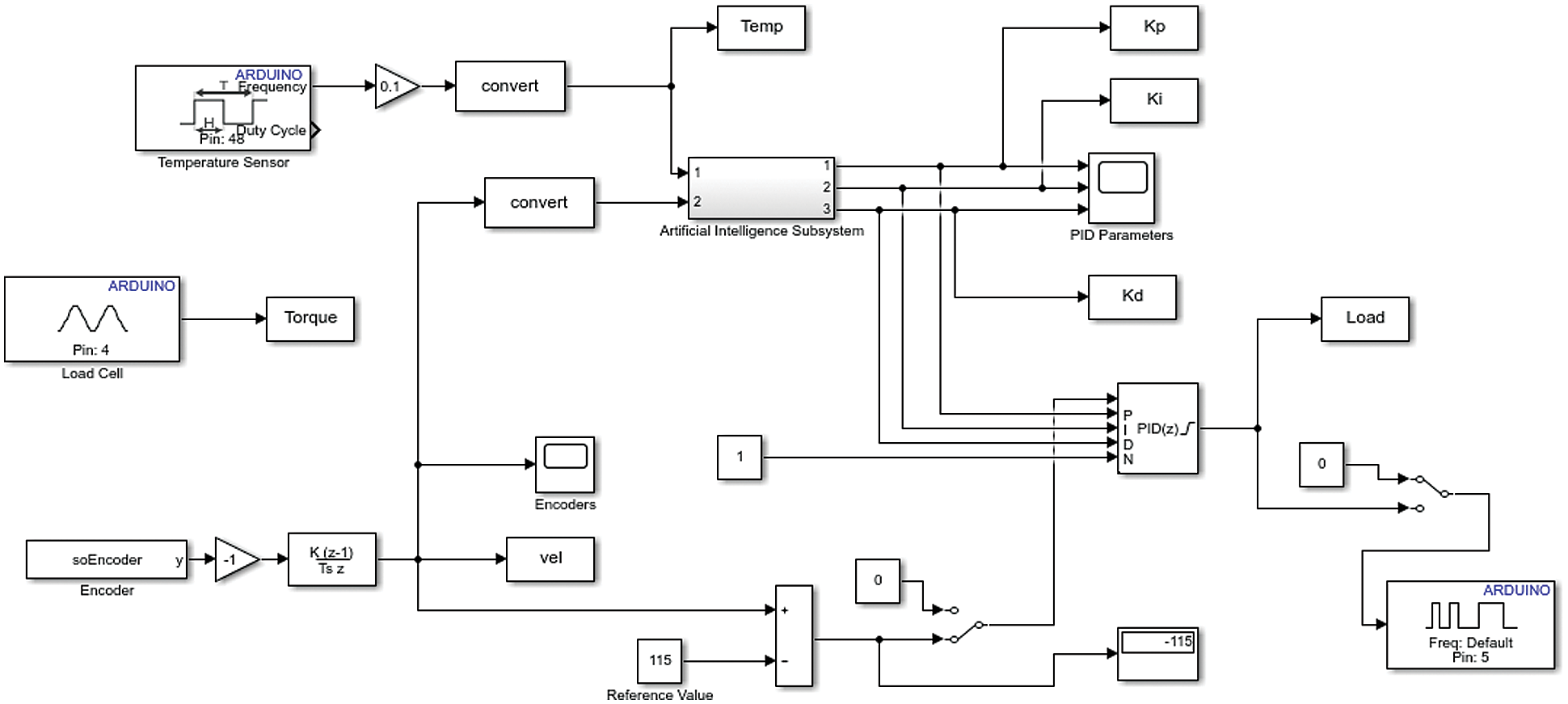
Figure 14: Real-time control diagram
Fig. 15 represents the validation results and parameters of designed control system. Shaft speed and temperature of the rotor selected randomly to observe the success rate of the adaptive PID system. The rotor temperature observed to be varying during the test. The range is between 41.6 and 56.9 while idle shaft speed is 125 (rpm/16) and reference speed is 115 (rpm/16). Accordingly, the artificial intelligence algorithms yielded Kp, Ki, and Kd has an interval of 4.61 and 4.88, 12.66 and 13.82, 3.16 and 3.45, respectively. Therefore, ECB braking load calculated using these parameters. At the end of the test, adaptive PID algorithms pause and magnitude of the parameters alter and rotor dissipates heat and decrease temperature consequently.
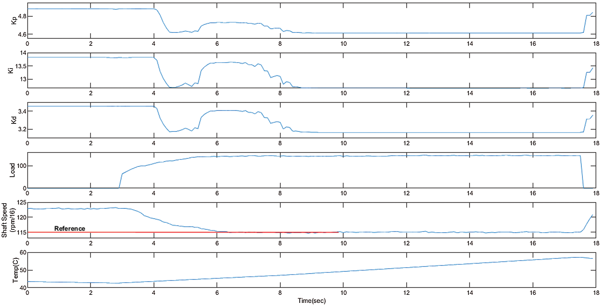
Figure 15: Validation test parameters and results
Eddy Current Dynamometers are electrically excited, non-contact brakes especially used for heavy-duty vehicles, and internal combustion engine testing with complications to control due to nonlinearities. In this paper, SHLNN + PID and ANFIS + PID GRNN + PID, and RBNN + PID control methods are examined for Eddy Current Dynamometer (ECD). For the Kp, Ki, and Kd values the most accurate algorithms are SHLNN + PID, RBNN + PID, and RBNN + PID with MAPE values of 0.43, 0.01, and 0.13, respectively. In this study, ideal NNs and the best PID parameters were found to be used in experimental studies. Therefore, the offered system is proven to be very useful as a tool for determining the correlation and also to control of Eddy Current Dynamometers. It also gives an accurate and simple approach in the analysis of this nonlinear, multivariable problem—that is, the robustness of the Eddy Current Dynamometer parameters.
Acknowledgement: I would like to acknowledge TEMSA and BAŞAK Truck Companies for their dynamometer, and IC engine grants.
Funding Statement: The authors received no specific funding for this study.
Conflicts of Interest: The authors declare that they have no conflicts of interest to report regarding the presented study.
1. A. H. Gosline and V. Hayward, “Eddy current brakes for haptic interfaces: Design, identification, and control,” IEEE/ASME Transactions on Mechatronics, vol. 13, no. 6, pp. 669–677, 2008. [Google Scholar]
2. B. J. Bunker, M. A. Franchek and B. E. Thomason, “Robust multivariable control of an engine-dynamometer system,” IEEE Transactions on Control Systems Technology, vol. 5, no. 2, pp. 189–199, 1997. [Google Scholar]
3. K. Lee and K. Park, “Optimal robust control of a contactless brake system using an eddy current,” Mechatronics, vol. 9, no. 6, pp. 615–631, 1999. [Google Scholar]
4. E. Simeu and D. Georges, “Modeling and control of an eddy current brake,” Control Engineering Practice, vol. 4, no. 1, pp. 19–26, 1996. [Google Scholar]
5. S. Anwar, “A parametric model of an eddy current electric machine for automotive braking applications,” IEEE Transactions on Control Systems Technology, vol. 12, no. 3, pp. 422–427, 2004. [Google Scholar]
6. K. K. Tan, S. N. Huang, C. S. Teo and R. Yang, “Damping estimation and control of a contactless brake system using an eddy current,” in IEEE ICCA 2010. Xiamen, China, 2224–2228, 2010. [Google Scholar]
7. S. Roozbehani, S. Saki, H. Nazifi and K. Kanzi, “Identification and fuzzy-PI controller design for a novel claw pole eddy current dynamometer in wide speed range,” in 24th Iranian Conf. on Electrical Engineering (ICEE), Shiraz, Iran, pp. 1038–1042, 2016. [Google Scholar]
8. J. Yang, F. Yi and J. Wang, “Model-based adaptive control of eddy current retarder,” in Chinese Control and Decision Conf. (CCDC), Shenyang, China, pp. 1889–1891, 2018. [Google Scholar]
9. X. Xu, T. Zhu, S. Chen and C. Wang, “Design and indirect adaptive fuzzy H∞ control of a novel retarder coupled with eddy current effect and MR effect,” Journal of Intelligent Material Systems and Structures, vol. 13, no. 6, pp. 640–660, 2020. [Google Scholar]
10. X. Jin, K. Chen, Y. Zhao, J. Ji and P. Jing, “Simulation of hydraulic transplanting robot control system based on fuzzy PID controller,” Measurement, vol. 164, no. 05, pp. 108023, 2020. [Google Scholar]
11. J. P. Moura, J. V. F. Neto, E. F. M. Ferreira and E. M. Araujo Filho, “On the design and analysis of structured-ANN for online PID-tuning to bulk resumption process in ore mining system,” Neurocomputing, vol. 402, no. 3, pp. 266–282, 2020. [Google Scholar]
12. G. Garima and P. Goswami, “Power quality improvement at nonlinear loads using transformer-less shunt active power filter with adaptive neural fuzzy interface system supervised PID controllers,” International Transactions on Electrical Energy Systems, vol. 30, no. 7, pp. 12415, 2020. [Google Scholar]
13. S. Kejian, L. Bin, W. Feiming, Z. Bin, L. Wei et al., “Research on the RBF-PID control method for the motor actuator used in a UHV GIS disconnector,” The Journal of Engineering, vol. 2019, no. 16, pp. 2013–2017, 2019. [Google Scholar]
14. X. Zhou, D. Li, L. Zhang and Q. Duan, “Application of an adaptive PID controller enhanced by a differential evolution algorithm for precise control of dissolved oxygen in recirculating aquaculture systems,” Biosystems Engineering, vol. 208, no. 23, pp. 186–198, 2021. [Google Scholar]
15. D. Ma, M. Song, P. Yu and J. Li, “Research of RBF-PID control in Maglev system,” Symmetry, vol. 12, no. 11, pp. 1780, 2020. [Google Scholar]
16. N. Hoang-Dung and H. Huynh, “Controlling the position of the carriage in real-time using the RBF neural network based PID controller,” in 18th Int. Conf. on Control, Automation and Systems (ICCAS), Pyeong Chang, Korea, pp. 1418–1423, 2018. [Google Scholar]
17. L. Nie, J. Guan, C. Lu, H. Zheng and Z. Yin, “Longitudinal speed control of autonomous vehicle based on a self-adaptive PID of radial basis function neural network,” IET Intelligent Transport Systems, vol. 12, no. 6, pp. 485–494, 2018. [Google Scholar]
18. A. Feroz Mirza, M. Mansoor, Q. Ling, M. I. Khan and O. Aldossary, “Advanced variable step size incremental conductance MPPT for a standalone PV system utilizing a GA-tuned PID controller,” Energies, vol. 13, no. 16, pp. 1–25, 2020. [Google Scholar]
19. S. Yıldırım, E. Tosun, A. Çalık, I. Uluocak and A. Avşar, “Artificial intelligence techniques for the vibration, noise, and emission characteristics of a hydrogen-enriched diesel engine,” Energy Sources, Part A: Recovery, Utilization, and Environmental Effects, vol. 41, no. 18, pp. 2194–2206, 2019. [Google Scholar]
20. A. K. Singh, I. Nasiruddin, A. K. Sharma and A. Saxena, “Modelling, analysis, and control of an eddy current braking system using intelligent controllers,” Journal of Intelligent & Fuzzy Systems, vol. 36, no. 3, pp. 2185–2194, 2019. [Google Scholar]
21. H. Yavuz and S. Beller, “An intelligent serial connected hybrid control method for gantry cranes,” Mechanical Systems and Signal Processing, vol. 146, no. 1, pp. 107011, 2021. [Google Scholar]
22. N. Zijie, Z. Peng, Y. Cui and Z. Jun, “PID control of an omnidirectional mobile platform based on an RBF neural network controller,” Industrial Robot: The International Journal of Robotics Research and Application, early access, 2021. [Google Scholar]
23. P. Aengchuan and B. Phruksaphanrat, “Comparison of fuzzy inference system (FISFIS with artificial neural networks (FIS + ANN) and FIS with adaptive neuro-fuzzy inference system (FIS + ANFIS) for inventory control,” Journal of Intelligent Manufacturing, vol. 29, no. 4, pp. 905–923, 2018. [Google Scholar]
24. E. Öztemel, Yapay Sinir Ağları, 1st ed., vol. 1. İstanbul, Turkey: Papatya Yayıncılık, 2012. [Google Scholar]
 | This work is licensed under a Creative Commons Attribution 4.0 International License, which permits unrestricted use, distribution, and reproduction in any medium, provided the original work is properly cited. |