Intelligent Automation & Soft Computing DOI:10.32604/iasc.2022.023712
Article

Criminal Persons Recognition Using Improved Feature Extraction Based Local Phase Quantization

P. Karuppanan1,* and K. Dhanalakshmi2

1Department of CSE, Pandian Saraswathi Yadav Engineering College, Sivaganga, 630561, Tamilnadu, India
2Department of CSE, PSNA College of Engineering and Technology, Dindigul, Tamilnadu, India
*Corresponding Author: P. Karuppanan. Email: prabukaruppanan@gmail.com
Received: 18 September 2021; Accepted: 26 November 2021

Abstract: Facial recognition is a trending technology that can identify or verify an individual from a video frame or digital image from any source. A major concern of facial recognition is achieving the accuracy on classification, precision, recall and F1-Score. Traditionally, numerous techniques involved in the working principle of facial recognition, as like Principle Component Analysis (PCA), Linear Discriminant Analysis (LDA), Subspace Decomposition Method, Eigen Feature extraction Method and all are characterized as instable, poor generalization which leads to poor classification. But the simplified method is feature extraction by comparing the particular facial features of the images from the collected dataset namely Labeled faces in the wild (LFW) and Olivetti Research Laboratory (ORL) dataset. In this paper, the feature extraction is based on local phase quantization with directional graph features for an effective optimal path and the geometric features. Further, Person Identification based deep neural network (PI-DNN) has proposed are expected to provide a high recognition rate. Various performance metrics, such as recognition rate, classification accuracy, accuracy, precision, recall, F1-score is evaluated. The proposed method achieves high-performance values when it is compared with other existing methods. The novelty of this paper explains in understanding the various features of different types of classifiers used. It is mainly developed to recognize the human faces in the crowd, and it is also deployed for criminal identification.

Keywords: Face recognition; face detection; criminal identification; local phase quantization (LPQ); directional graph; deep neural network

1  Introduction

Face recognition can also be defined as biometric artificial intelligence relied on the application that is exclusively designated to recognize a person by exploring sequences based on the individual’s facial shape and texture. Even though facial recognition has a wide variety of applications, it is typically essential to use it in the detection of criminal and forensic investigations and inquiries. Applying the digital images for the identification of victims can be challenging at specific occasions. Especially when the individual is wearing a mask or tattoo, or if the environment has background noises, camera distortion, insufficient storage, inadequate computing techniques, occlusion, detection of identical images and low-resolution images [1]. Nowadays, deep learning explored the hidden sights of advanced computing applications and executed it in the right place to get an efficient expected output. It is trained similar to the human brain to analyze multiple human faces and store it in a database for future use. Generally, human utilizes all his sensory organs to recollect and analyze the input data, a similar computer process, and the input captured images into various features by a different algorithm. To get the exact desired result and confirm it by comparing it with the original picture by an integral section of biometrics and matching of essential traits. The system involved dual methods, such as face detection and face recognition [2]. Face detection is used to search and find one face by image processing, and face recognition is performed by comparing and analyzing the processed image with similar images from the database.

The method of face recognition in the proposed research comprises feature extraction and feature classification methods. In feature extraction, Phase quantization, directional graph-based process, and Geometric based feature extraction are performed. The feature classification is achieved by using Convolutional neural network (CNN) for criminal identification. The mandatory methods for effective facial recognition should calibrate the facial expression from the given images. The facial expression can be derived from eyes, mouth, eyebrows, cheeks, and it’s represented as salient regions. But few emotions like surprise and sadness acquired with only one salient feature, but anger and fear cannot be obtained from a single salient feature. In feature extraction, Phase quantization is applied to extract the features from blurred images by short Fourier transform to analyze the structural properties of the image with promising values of accuracy and efficacy [3]. Directional graph-based and geometric based methods in feature extraction are applied to extract the facial feature in Region of interest (ROI) along with error filtering techniques to provide prominent face components. It is used to locate the edges and relative size and position of mandatory expression components such as mouth, eyes, nose, and eyebrows. Then it is differentiated into the unimportant and meaningful part and also the conversion of grayscale distribution into feature vector based on the value of the pixel. The feature extraction is based on image pixel distribution, orientation selectivity, and spatial localization. The extracted images are then fed into CNN for further classification by deep learning. It is composed of multiple layers to detect necessary edges, intricate shapes, and by further processing, the final layer can catch the entire face and confirm it by verifying with the high dimensional dataset. Hence it is mostly preferred in real-time applications.

Face Recognition is mainly deployed in genetic engineering and biometric devices for identification, authorization, verification, and authentication. Many companies have adopted face recognition for security purposes by implementing CCTV to manages and control the organization. Apart from security system, it have other exciting applications such as unlocking the phones, more refreshing advertising, finding missing people, protecting the law enforcement, identifying person on social media, diagnosing various types of diseases, spotting VIP at events, protecting school and government institutions from threat, and controls the access to sensitive regions. In recent days Deep learning techniques are highly utilized in recognition of human face from the large datasets [4]. By considering this the major contribution of the study involves,

•   The applied machine learning algorithm, such as Local Phase quantization with directorial graph-based features and Geometric based feature extraction have been applied in selected LFW and ORL datasets to perform effective human face recognition.

•   To find the optimal path to achieve the best features using directional graph-based features.

•   To implement the Person identification based Deep Neural network considered an effective classifier and applied in the real-time dataset for criminal identification.

The organization of the research is as follows. Section 2 explains the related work of face recognition on different feature extraction and classification methods. Section 3 is based on the detailed description of the proposed work. Section 4 represents the analysis of the performance of the proposed method, and Section 5 concludes the results of the research work and explains its future extension of the work.

2  Literature Review

In modern ages, face recognition has achieved extensive attention from research and market, but still, it has some challenging task to implement in real-time applications. In past decades, a wide variety of face recognition machine algorithm is developed. But the proposed techniques in feature extraction and classification achieves high accuracy in face recognition. The paper is based on CNN in an image recognition process for the input of the Gait energy picture. It is composed of dual pattern trios’ images of pooling, convolutional, and normalization cover and double connected layers with high efficacy. Classification is the last stage of the face expression recognition where the classifier divides the expression like sad, smile, surprise, fear, anger, neutral and disgust. This method involves silhouette extraction, extraction of features, and matching of images [5,6]. The silhouette extraction is made to avoid being affected by clothing, texture, and color. Then the Gait energy image (GEI) picture is fed into CNN of 88 * 128 pixels [7]. The face recognition method involves face area acquisition, localization, and segmentation to define the facial expression, face shape, and position of components, and the quality of the image [8]. Then feature detection and extraction of the face are obtained by geometric approach by designing feature vectors to locate the corners of the various face feature components. Then it is fed as the input image for the backpropagation neural network model for facial expression recognition. But this method fails to work if there is any alteration in eye areas [9].

The link prediction in face recognition is divided into two types, such as feature extraction and feature learning methods. Similarity-based methods, probabilistic methods, and likelihood-based methods fall under feature extraction techniques. In similarity-based models, it follows global, local, and Quasi-local approaches by calculating the similarity between nodes. Depending on the structure of the network, a statistical model is designed to calculate the possibility of unnoticed connections to happen by using maximum likelihood models such as Hierarchical structural design and stochastic block model. These techniques are time-consuming and derive an accurate result. In feature learning methods, CNN extract features from the graph to check the connection between linked nodes and extract the data from the topology of the system [10]. The awareness of this learning model is to establish the structure of the localized neighbor by disintegrated feature data as an alternative to creating the entire graph by multiple source link prediction of input images [11]. The detection and localization of blurred face using local phase quantization applying Fourier transform phase in resident neighborhoods [12]. Under certain conditions, the period can be represented as a blur invariant attribute. So in the analysis, a histogram of local phase quantization labels calculated in resident areas is executed as face descriptor, related to broadly applied local binary pattern for a description of face images. But to limit the impact of lighting alteration in face pictures, procedure on illumination normalization is applied that comprises of contrast equalization, gamma correction, and Gaussian filtering that increases the result of recognition accuracy [13]. Some investigations made on a pair of parent and child to verify the effectiveness of the local phase quantization. The standardized and cropped images of parent and child were fed as input and converted to grayscale. Then local phase quantization is applied to retrieve the local features of every mode [14]. Encrypted images are differentiated into k non-overlap rectangle scratches, and histogram values define each stretch. Each histogram has allocated to the high dimensional feature vector. Then cosine similarity is analyzed between the images by projecting into transformed subspace, and the resultant score is compared with threshold value from Receiver Operator Characteristic (ROC) by performance measures. With the obtained result, it is decided whether the person belongs to the same family or not [15]. The face is an essential attribute considered in a security system. Even though it is applied vastly, there is some limitation such as illumination, pose, and condition of the pictures [16]. To overcome this issue, face recognition is performed under non-uniform illumination by CNN that can learn exclusively local patterns from information is utilized for identification of a face. The symmetry of face data is processed to eliminate and enhance the performance of the system by accepting the horizontal reflection of the face images. The experiment was made using the Yale dataset under various illumination settings and showed moderate enhancement in the performance of CNN. The production remains undisturbed by the horizontal reflection of images. But it is failed when it is applied with fisher discriminant analysis and fisher linear discriminant analysis that is based on Gabor wavelet transform. Human gait is soft biometric that support to identify an individual by their walking gestures [17]. This research focused on deep neural network for the effective face recognition system in which the new face alignment technique has been implemented for face key point localization. The deep features dimensionality has reduced by the principal component analysis for removing the contaminated and redundant visual features. The feature vectors similarity has been evaluated by Bayesian context and the better classification accuracy attained. Different face recognition attacks have been handled based on different frameworks. [18] Personal face images have been differentiated by Deep Face. 4000 unique identities have been verified in this study. Deep convolutional neural networks have been used for learning the deep identification DeepID. This study utilizing the LFW dataset. [19] AlexNet network has been utilized to evaluate the ORL dataset for realizing the face recognition. The proposed convolutional kernel network with recognition rate depicts higher rate compared with AlexNet network in face recognition. The gender-based classification is also made possible using a supervised machine learning approach. The diverse classifier used in this approach is the support vector machine, convolutional neural network, and adaptive boost algorithm. The input images are fed into pre-processing for removing noisy information, and feature extraction is based on a geometric approach to extract meaningful data from the processed images. It is fed into the combination of a classifier to get the resultant output. It is used to recognize the gender of the picture.

3  Proposed Methodology

In the proposed work, the features from the image are extracted using Local phase quantization based on directional graph features and geometric based features and classified using Person identification based Deep Neural Network (PI-DNN) whereas it is not found in previous texture and feature extraction algorithms like edge based method, geometric feature-based method, texture feature-based method, patch-based method, global and local feature-based method. Gabor filter, Vertical Time Backward, Gaussian Filter, Weber Local Descriptor. Supervised Descent Method Discrete Contourlet Transform, Graphics-processing unit based Active Shape Model, Principal Component Analysis (PCA), Independent Component Analysis (ICA) and Local Binary Pattern (LBP) are the text descriptors. In this study further, the criminal faces are identified from the selected LFW and ORL datasets using the proposed model shown in Fig. 1.

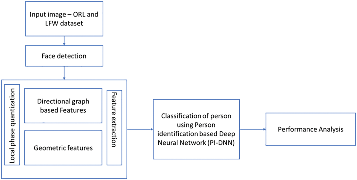
Figure 1: Architecture of proposed system

3.1 Local Phase Quantization for Feature Extraction

In general, Local Phase quantization is insensitive to centrally symmetric texture images. So this research considered both spatial and temporal coordinates. In statistical analysis, to overcome the loss of generality, the covariance matrix and cross-correlation are evaluated for the transformed coefficients. This method is based on the property of blur invariance of the Fourier phase spectrum. It utilizes local phase data that is derived using a two-dimensional discrete Fourier transform or Short-Term Fourier Transform(STFT) calculated on a rectangular matrix M × M at each pixel position x of image f(x). It can be formulated as below Eq. (1),

F(q,a)=∑b∈Na⁡f(a−b)e−j2πqTb=wqTfa (1)

Here, wq represents the basis vector of frequency q. fa Vector represents all image samples from neighborhood Na.

Local Phase quantization is defined as follows,

The original image is compared with the input image, and it is formulated as follows,

g(a,b)=f(a,b)⊗h(a,b)+n(a,b) (2)

From Eq. (2), where h(a, b) is represented as a Point Spread Function (PSF), n(a, b) is described as an additive noise, then the Fourier transformation is performed to convert the image from the range of high intensity to low intensity. It is formulated as below,

G(m,n)=F(m,n).H(m,n) (3)

From Eq. (3), where G(m, n), F(m, n), H(m, n) Fourier are transforms of g(a, b), f(a, b), and h(a, b) respectively. In order to predict the intensity range of an image, phase information and magnitude can be extracted as follows,

∠G(a,b)=∠F(a,b)+∠H(a,b) (4)

From Eq. (4), where ∠G(a,b),∠F(a,b),∠H(a,b) are phases of g(a, b), f(a, b), and h(a, b) respectively.

To analyze the impulsive response of an image, Point Spread Function is calibrated as below,

∠H(a,b)={0,ifH(a,b)≥0π,otherwise, (5)

To calculate the relative translation between two pixels, phase correlation is estimated as below,

∠G(a,b)=∠F(a,b),for allH(a,b)≥0. (6)

Then, Short Term Fourier Transform is executed at first to extract phase information for every pixel. It can be calculated as below,

G(a,b)=∑a∈Nb⁡∑b∈Nb⁡g(a,b)e−j2π(ma+nb)M (7)

The final results are organized as below,

V=[G(m1),G(m2),G(m3),G(m4)] (8)

and

W=[Re{V},Im{V}] (9)

From Eq. (9), where Re{V}, Im{V} represent real and imaginary parts correspondingly. Lastly, the encoded value (x) distribution histogram within an image is built to attain the local phase quantization in two hundred and fifty six dimensions. It is given by the below Eq. (10).

x=∑i=18⁡qi2i−1 (10)

Here qi denotes the quantization corresponding to the ith element in W and is given by the below Eqs. (11) and (12).

qi={1,ifWi≥00,otherwise (11)

Ga= VTFa∑i=0N−1⁡f(i)g(a,b) (12)

Though, the local quantization measures the short-term Fourier Transform coefficients, this strategy tends to confirm the blur insensitivity with a slight minimum discriminative power. On the other hand, it is just an indication of STFT coefficients that impact the texture characterization.

3.1.1 Directional Graph-based Features

In this process, the input image is represented as a graph where each pixel in the picture is mapped as times series of respective vertex [20]. In this context, the image retrieval concept rely on the Graph Theory (GT). Moreover, the edge detection is implemented as an alternative to the map based representation. The main aim of the edge concentration is to obtain the rapid alterations in the brightness of the image. This representation permits a direct accessibility to the picture’s edge node without segmentation and edge point search. Another advance is less data consumption; only data for nodes and their connections are needed, which is important in large database applications for good scalability. Typically, a time series {xi}(i=1,…,n) is mapped into a graph G(V, E) where a time, Point xi is mapped into a node vi ∈ V. The relation between any two points (xi, xj) is represented as an edge eij ∈ E, and the value is defined as below,

eij={ 1, xk<xi∧   xk<xj    ∀k∈(i,j)∧i<j 0, otherwise (13)

From Eq. (13), Where eij implies the presence of edge. If eij = 0, implies that the edge does not exist. There are several steps in assessing directional graphs, which are explained further.

Directional Graph Generation:

Step 1: Link Density for Directed Graph

The increase in the number of edges increases the graph density. It can be formulated as below,

Edges = size(Eij)    // Number of formed edges,

vertices  =  size (Vij)   // Number of formed vertices,

Densegraph=2∗Edgesvertices(vertices−1) (14)

Step 2: Average of closeness centrality

The graph can effectively detect the nodes centrality that have capability to spread the information by calculating the closeness of centrality. It can be formulated as below,

Closenesscentral(a)=size(Eij)D(a) (15)

where, D (a) = lima→1:size(Vij,1)⁡∑b=1size(Vij,1)⁡Dist(a,b) ;

Dist (a, b) = limb→1:size(Vij,1)⁡(X(Vij(a))−X(Vij(b)))2

Step 3: Graph Entropy

To characterize the texture of input image, graph entropy is calculated. It can be formulated as below,

Entropy=−∑i=1n⁡P(i)∗log(P(i)) (16)

where,

P-Degree Distribution of graph, P = nkn

nk-number of k connected nodes to the particular nth node.

n-Number of vertices

Step 4: Average Distribution Weight of the Graph

To detect the similarities or dissimilarities between the vertices connected by the edges, weight is calculated using the below Eq. (17),

Weightavg=mean(W) (17)

From Eq. (17), where W can be represented as the weight of all edges in a graph.

Step 5: Graph Hilbert Transform (GHT):

To convert the image and to extract the global features, the Hilbert transform method is applied in this work. The Hilbert transform of the graph of a function f(x) can be defined as below,

F(t)=1π∫−∞∞f(x)t−xdx (18)

When Hilbert transform is computed in more than a single dimension and if any of the dimensions remain unchanged (constant), then the transform will be a numerical value near to zero or zero. Thus, the Hilbert transform corresponding to the constant is 0.

3.1.2 Geometric Features

In a geometric-based approach, the local features that are based on local statistics and locations like bodily features are extracted. It can be implemented in the following ways.

•   Convex Area Of Image

•   Eccentricity

•   Filled Area

•   Axis Length

•   Orientation

Convex Area of Image

The binary image covering the convex area gives the outline of the curved image. The convex area can be denoted as several pixels in a convex image. The convex area can be computed as shown in Fig. 2.

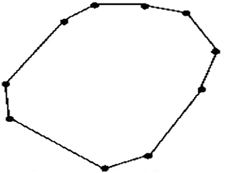
Figure 2: Convex area of image

The Eccentricity of an Image

Eccentricity is the ratio of length off short or minor axis to the length of the major or long axis of an image. For a linked region of a digital image, it is defined by neighbor graph and calibrated metrics. The number that measures and look of the ellipse by illustrating its flatness is also called as eccentricity. The eccentricity can be calculated by using the given equation,

eccentricity=lenghtoftheshortaxislengthofthelongaxis (19)

Filled Area

Full Image can be denoted as a binary image of the same size similar to the bounding box of the region. Filled Area is defined as the number of pixels in that particular filled image.

Length of the Major Axis

The long line’s endpoints denotes the major axis. It is constructed through an object or an image. These endpoints are retrieved by computing the distance of the pixel amongst individual boundary pixel grouping in the boundary of an object. It also determines the pair with an improved length. The length of the major axis affords the object length or image value.

Length of the Minor Axis

The minor axis endpoint is the longest line that can be constructed through the image or object, whereas remaining perpendicular along with the major axis. Minor Axis Length gives the value of the image or object width.

Orientation

The angle of the major axis is computed from an angle amongst the major axis and X-axis of the corresponding image. It can differ from 0° to 360°. Orientation refers to the overall direction of the object shape in an image.

3.2 Deep Neural Network for Person Identification

The proposed architecture is based on deep neural network for the person identification (PI-DNN) shown in Fig. 3. From the geometric based feature vectors and local phase quantization, the input is accepted from the PI-DNN. Fully connected dense nodes of 512 comprised in dense layer which are included after the input layer. The dense layer output has expressed as,

H1−U.V (20)

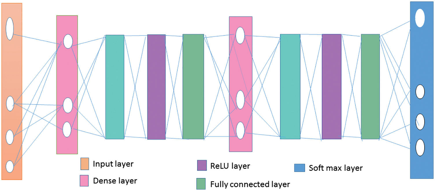
Figure 3: PI-DNN architecture

From the above Eq. (20), V-dimensional weight matrix of 25 × 512. At every epoch, A batch has been selected and the size of A is T. The H1 dimensional is then calculated as T × 512.

The over-fitting is prevented and the performance, stability and speed have been improved by the batch normalization layer inclusion after dense layer. The A mean measured at batch normalization layer is measured as,

σA−1T∑T−1T⁡H1(t) (21)

From Eq. (21), H1(t) is defined as Tth row vector of H1 and 1 × 512 resulted as the σA dimension. The A variance with σA measured as,

−γA2−1T∑T−1T⁡{H1(t)−σA}2 (22)

From Eq. (22), 1 × 512 is the γA2 dimension.

Let consider H1(t, u) as the H1(t)’s uth element is the σA and γA2(u) ’s uth element and it is the γA2 ’s uth element. Further, normalized H1(T, u) resulted in,

H1(~t,u)−H1(t,u)−σA(u)γA2(u)+ε (23)

From Eq. (23), t ε { 1, 2, …. , T − 1, T}, u  ∈ {1, 2, …., 511, 512} and small constant value is termed as ε included for numerical stability. ε = 0.001 value is set.

In the batch normalization layer output, H1(~t,u) is termed as,

H2(t,u)−λ(u).H1(~t,u)+μ(u), (24)

From Eq. (24), the parameters μ(u) and λ(u) have been learned during the training phase based optimization process.

In the proposed PI-DNN model, after the batch normalization layer the activation layer is included. The rectified linear unit activation function-Rectified Linear Unit (ReLU) is utilized at an activation layer which are established for adding non-linearity to proposed PI-DNN model. The activation layer output is expressed as,

H3(t,u)−max(H2(t,u),0), (25)

From Eq. (25), max(H2(t, u), 0) is considered as function which returns a for the H2(t, u) > 0 and 0 otherwise.

Dropout layer is included after the activation layer. At the drop out layer, during the training phase, at specified rates the input units have been dropped randomly. The dropout rate is 0.1 in PI-DNN proposed model. As explained above, batch normalization layer, second dense layer, dropout layer and activation layer have been added successfully. Dense nodes in first dense layer is similar as such in the second dense layer. ReLU activation has utilized at second activation layer. In second drop out layer, dropout rate is 0.1. For every person, the classification of labels is included in soft max layer at PI-DNN end of the model. As an activation function, the softmax function has been performed in this layer. Hence, from softmax layer, activation values have been normalized through

Zθ~−exp⁡(Zθ)∑θ−1θ⁡exp⁡(zθ),∀θε{1,2,…θ−1,θ} (26)

From Eq. (26), where exp(.)-exponential function, label- θ for θ th person. The normalized activation value is Zθ~ and the un-normalized activation values are Zθ. The total number of labels are θ, if the dataset of person identification comprised with total subjects. 1×θ dimensional vector refer as softmax layer output in which the vector θ th value is Zθ~. Sparse categorical cross entropy loss property is applied to an objective function for PI-DNN training.

4  Performance Analysis

The experimental analysis is performed by calculating various performance metrics such as accuracy, precision, recall, F1-score, classification accuracy, and recognition rate. It is verified with a different existing method such as FaceNet, Clinical Document Architecture (CDA), Transform and Two Dimensional Logarithmic (TDL) algorithm k class feature transfer KCFT, Gabor-Based Feature Extraction and Feature Space Transformation (G-FST), and Support Vector Machine (SVM) classifier trained with Histogram of Oriented Gradients (HOG) features and image segmentation (HOG + SVM) () by using LFW and ORL dataset. The criminal images are also analyzed to identify the criminals in the images using the proposed model.

4.1 Dataset Description

•   Labeled Faces in the Wild (LFW) dataset contains 13,000 images to study the problem of unconfined face recognition, and it is detected by Viola-Jones face detector. The LFW dataset is obtained from http://vis-www.cs.umass.edu/lfw/.

•   ORL dataset contains the pictures captured from 1992 to 1994 of different subjects under various lighting conditions with several facial expression such as open or closed eyes, smiling and not smiling. The ORL dataset is obtained from https://paperswithcode.com/dataset/orl.

4.2 Recognition Rate

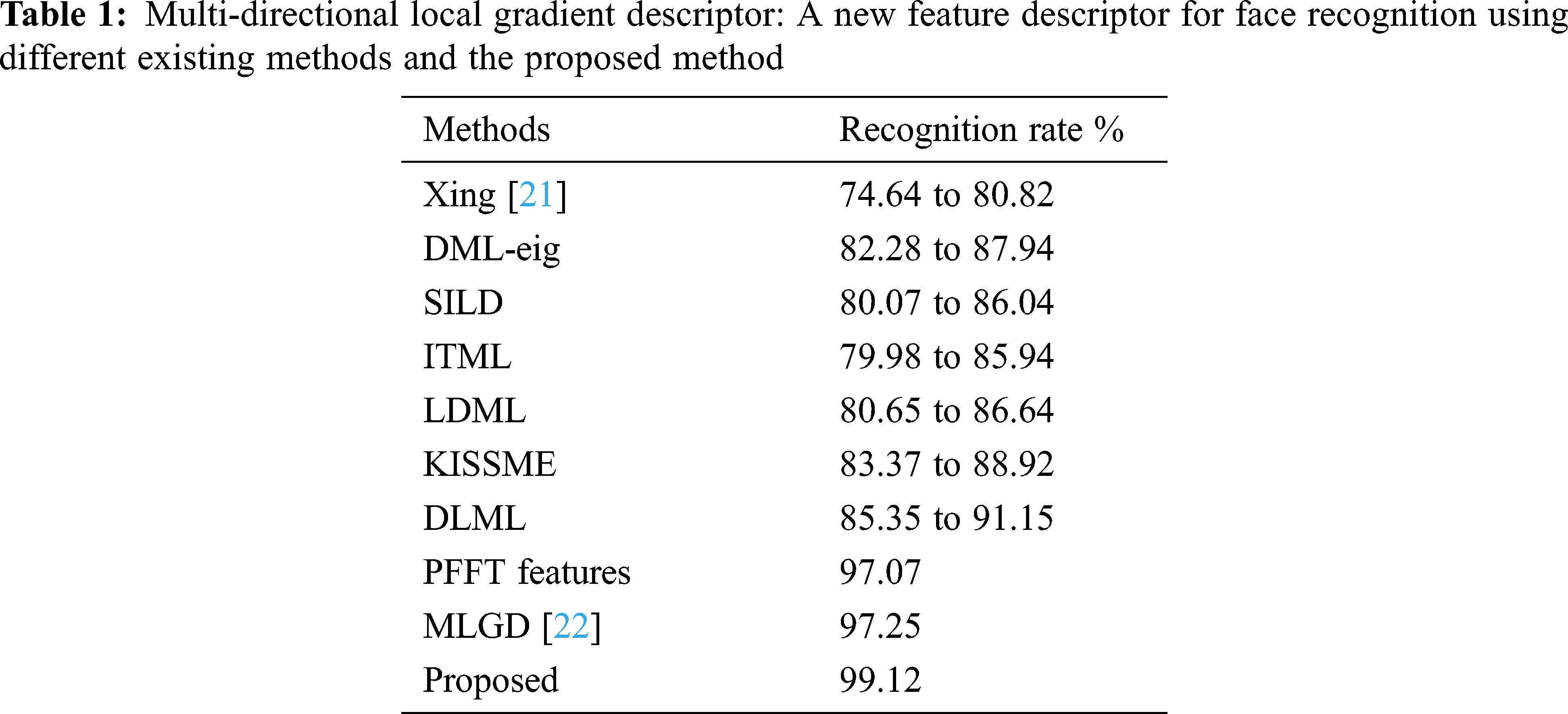
The recognition rate is divined as the summation of correctly identified acquisition image by total number acquisition images by various experimental analysis. Tab. 1 shows the exploratory analysis of the recognition rate for the proposed and different existing methods is shown.

4.3 Classification Accuracy

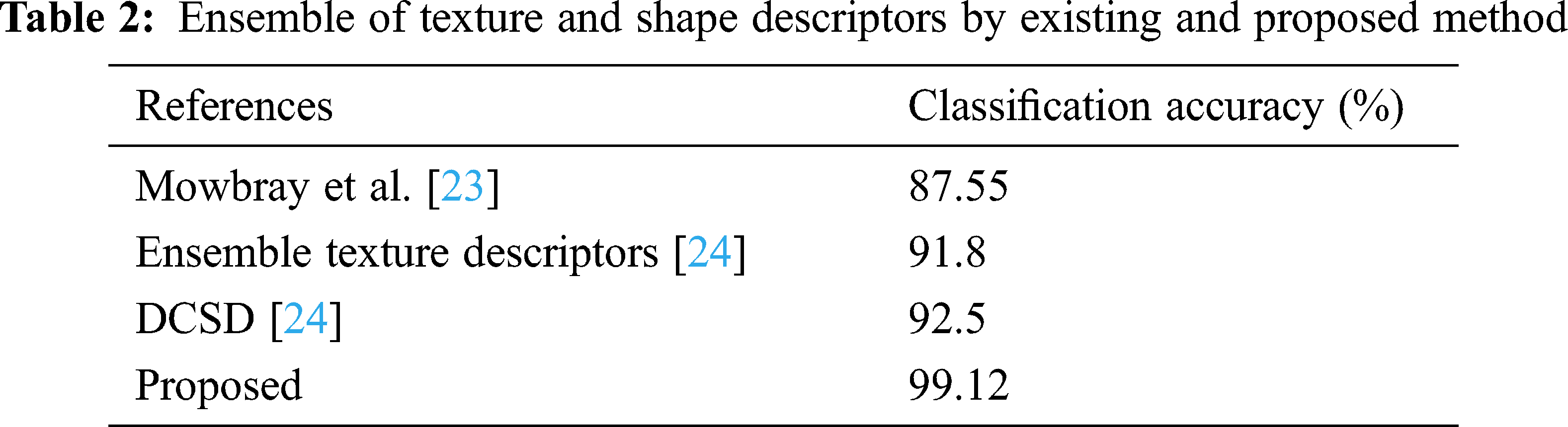
Classification accuracy is defined as the ratio of total quantity of accurate prediction images to the total quantity of input images by using various experimental analysis. Tab. 2 shows the result of classification accuracy by using existing and proposed methods. It is proved that the proposed method gives give the value of accuracy.

4.4 Accuracy

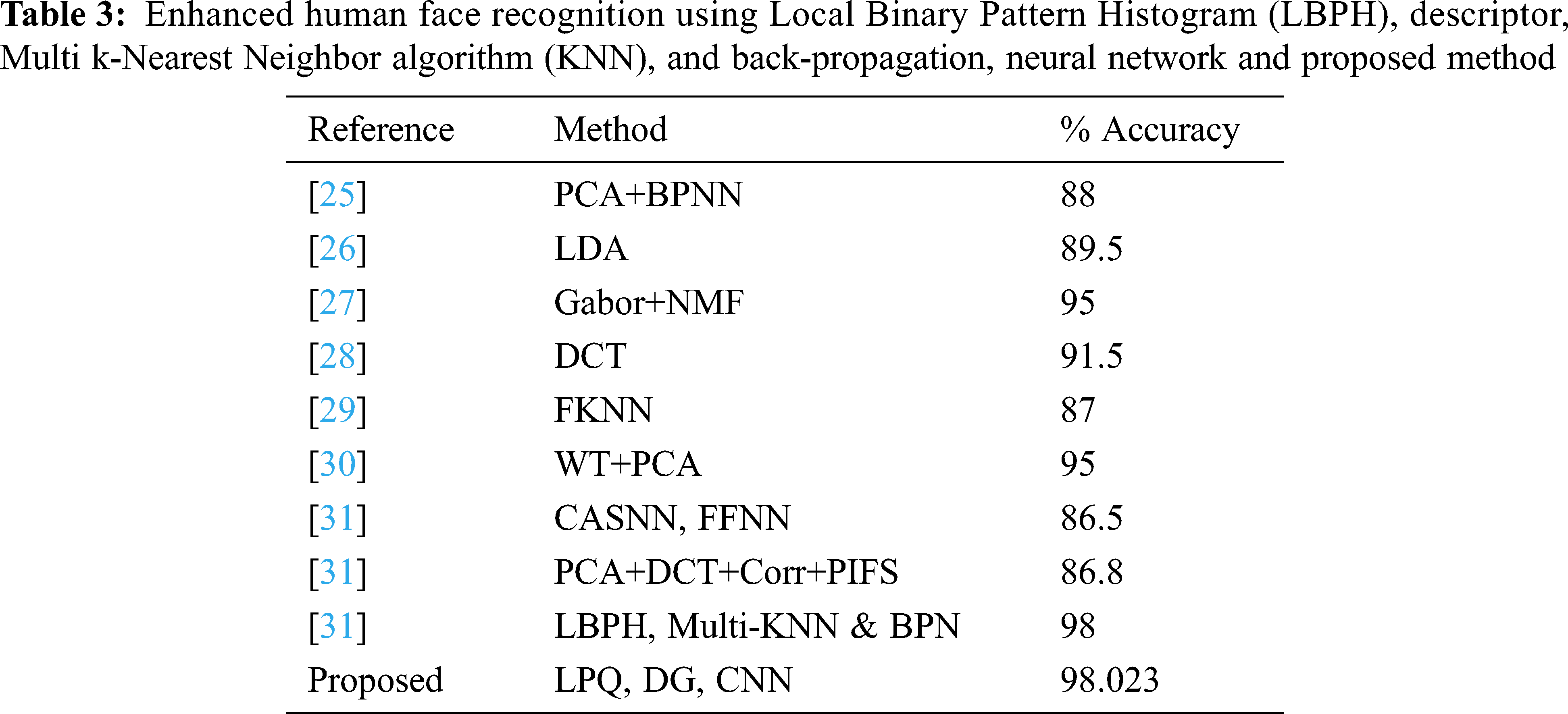
Accuracy is computed to validate the proposed system’s performance metrics. It is shown in Tab. 3 that the proposed method gives high efficiency when compared with another existing method. From the Figs. 4 and 5, it is shown that the value of accuracy is high in the proposed method using a realtime dataset from the image Fig. 8 and compared to other existing methods such as FaceNet, CDA, TDL, KCFT, G-FST, and HOG + SVM by using LFW and ORL dataset.

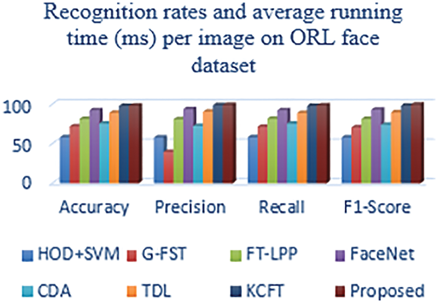
Figure 4: Comparison of performance metrics using the different existing method and proposed method in ORL dataset

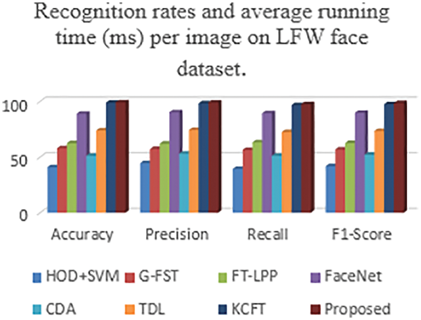
Figure 5: Comparison of performance metrics using the different existing method and proposed method in LFW dataset

4.5 Precision

Precision is a significant performance metric calculated to find the positive predicted values. It is the fraction of related instances from the extracted cases. From the Figs. 6 and 7, it is shown that the value of precision is high in the proposed method using a real-time dataset from the image Fig. 8 and compared to other existing methods such as FaceNet, CDA, TDL, KCFT, G-FST, and HOG + SVM by using LFW and ORL dataset.

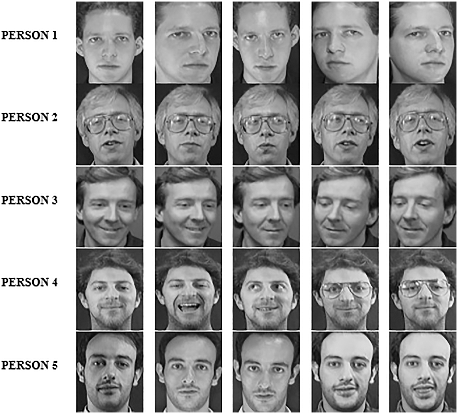
Figure 6: ORL dataset of various person

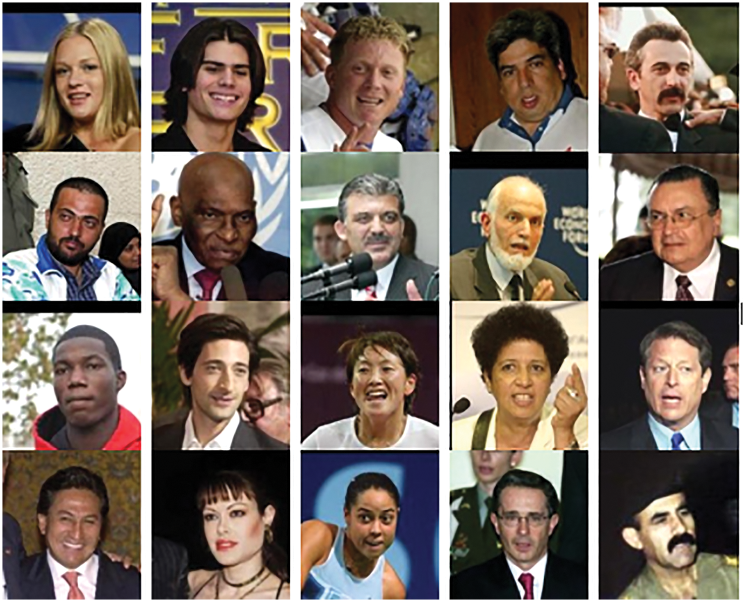
Figure 7: LFW dataset of various person

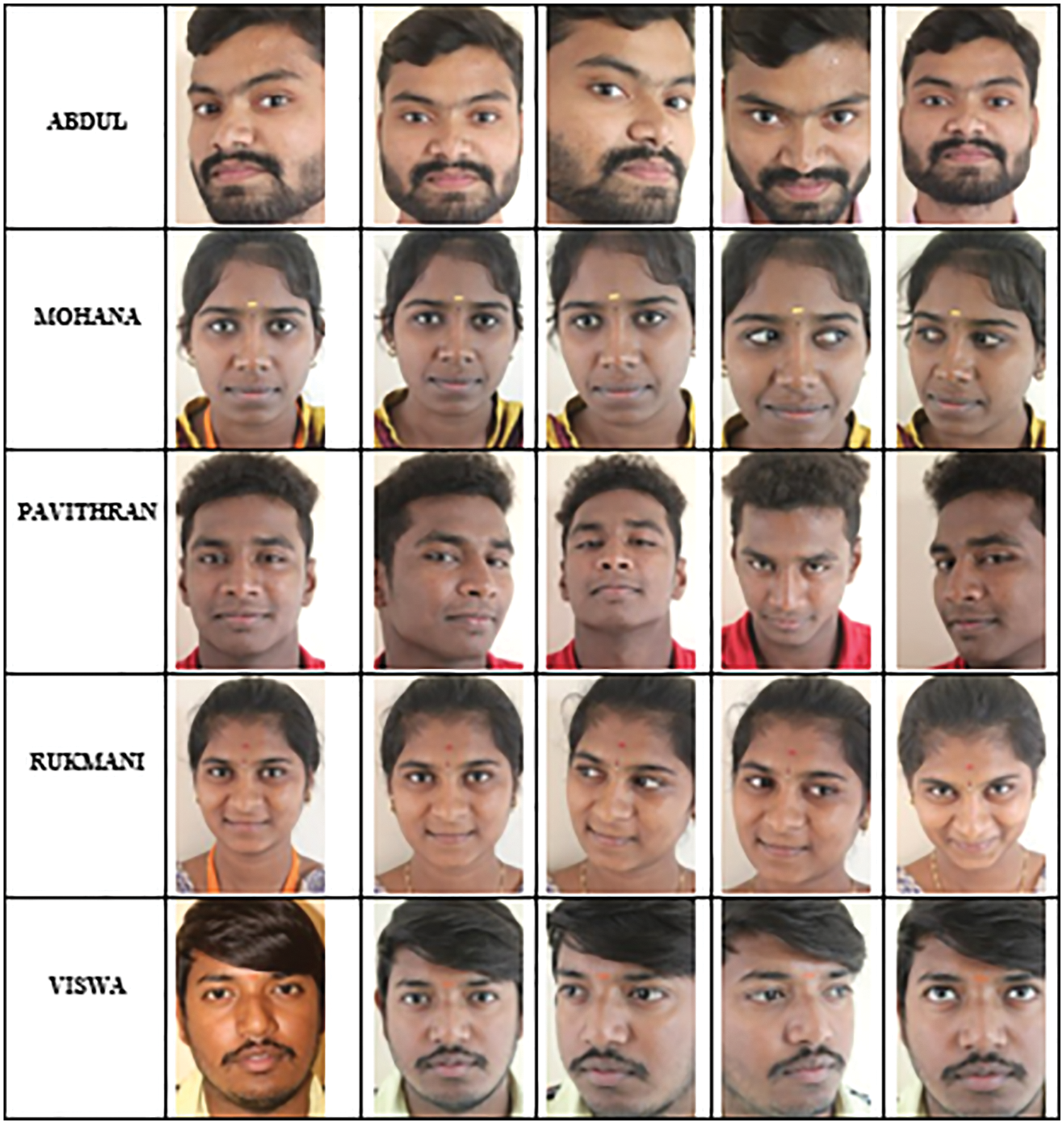
Figure 8: Real-time datasets of various person

4.6 Recall

The recall is termed as sensitivity that is the ratio of total quantity of related instances that are truly retrieved. From the Figs. 9 and 10, it is shown that the value of recall is high in the proposed method using real-time dataset from the image and it is compared to other existing methods such as FaceNet, CDA, TDL, KCFT, G-FST and HOG + SVM by using images of ORL and LFW dataset

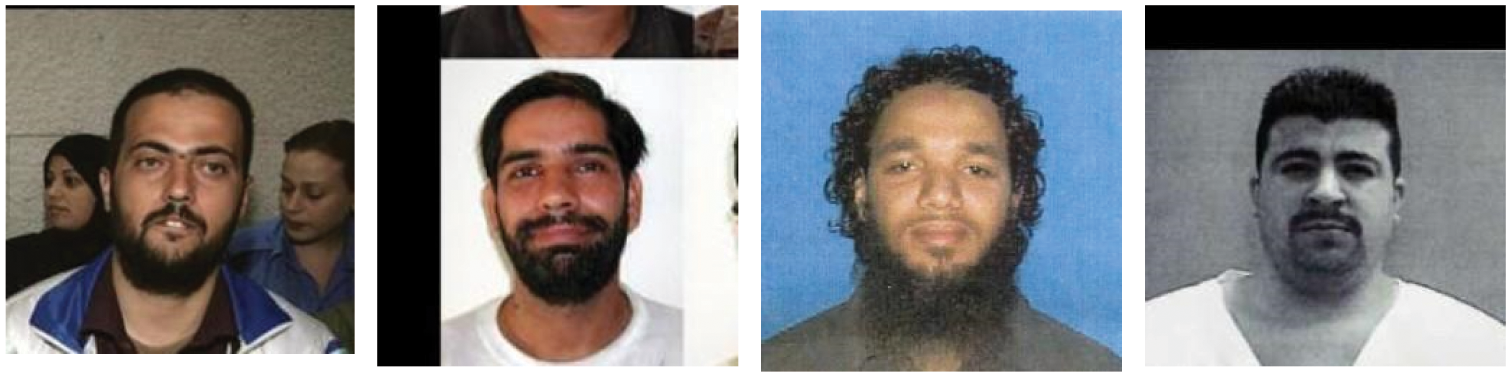
Figure 9: LFW criminal dataset

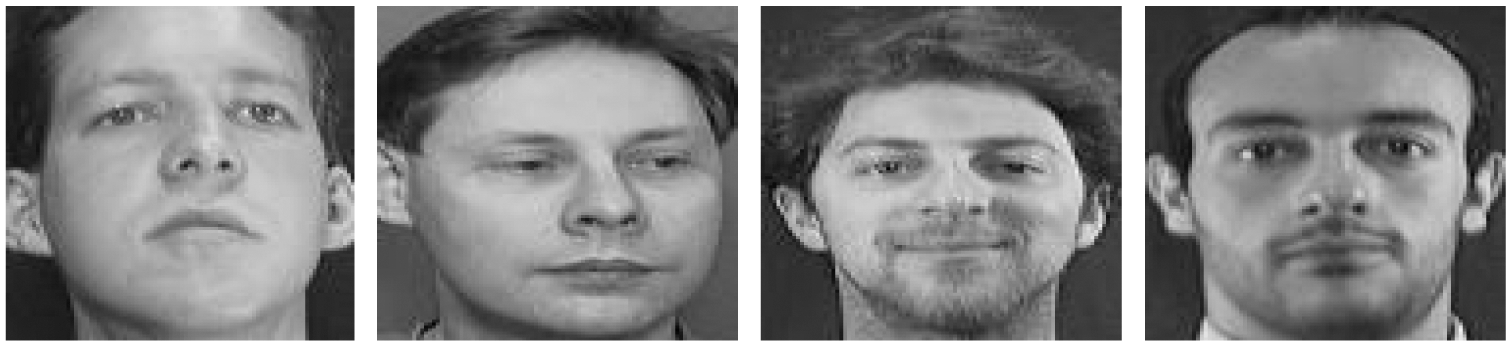
Figure 10: ORL criminal dataset

4.7 F1-Score

It is one of the critical performance metrics to test the accuracy of the proposed method. It is shortly defined as the weighted harmonic mean of tested values of recall and precision. It is observed that the value of recall is high in the proposed method by using input real-time dataset images from the Fig. 8. It is compared to other existing methods such as FaceNet, CDA, TDL, KCFT, G-FST, and HOG + SVM by using the pictures of ORL and LFW dataset.

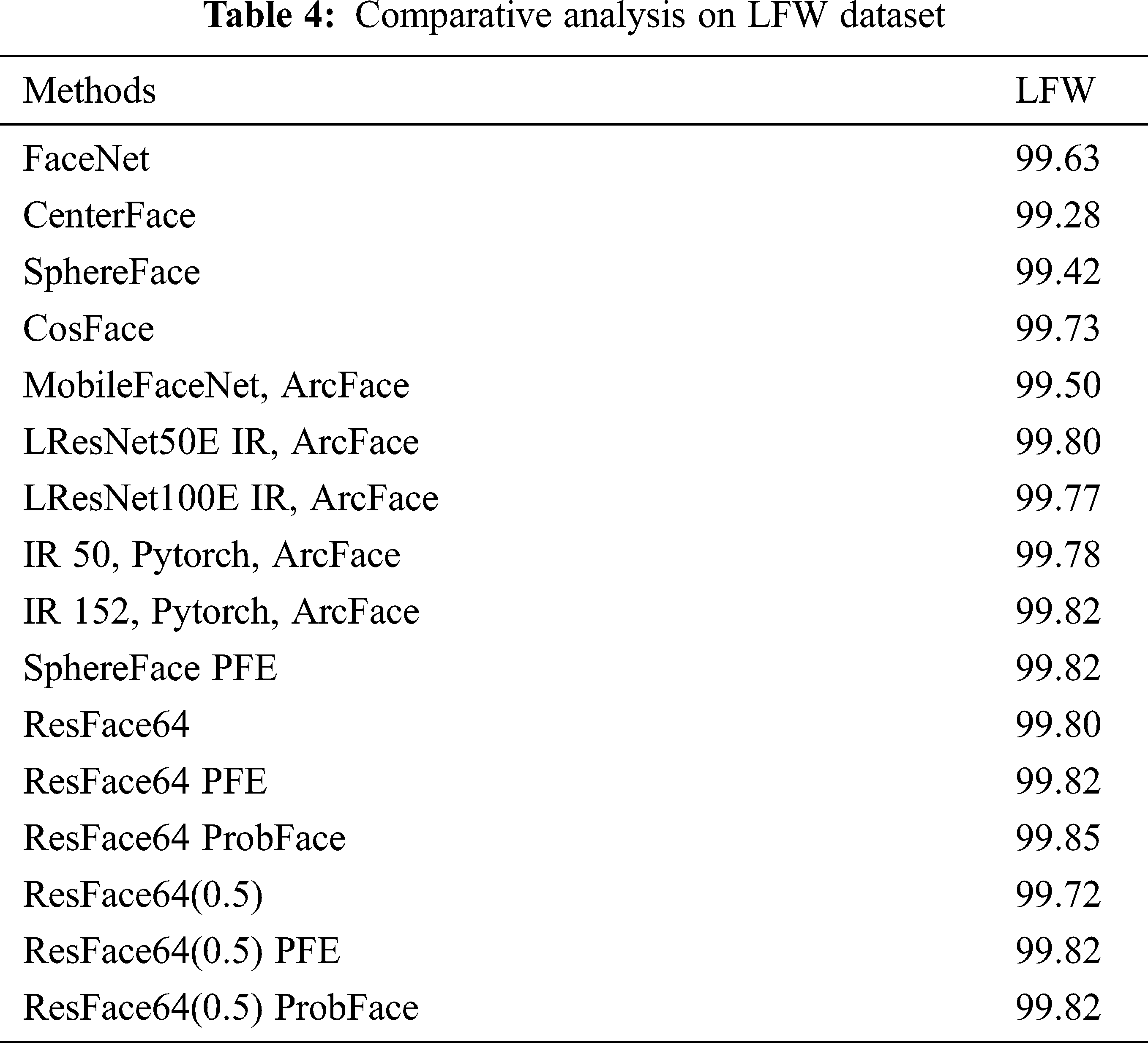
4.8 Comparative Analysis Results Based on Criminals Identification on LFW and ORL Datasets

From the below Tabs. 4 and 5 it shows the comparative analysis of the proposed Multi-directional local gradient descriptor with DNN and existing methods [32] based on LFW dataset. The standard models are resolution face (resface) (0.5) and resface64. The existing models from earlier state of art researches are analyzed and compared with proposed model. The basic model is FaceNet [33] and in LFW, it shows accuracy as 99.63%. Further, Sphere Face [34] and Center Face [35] shows lesser results because they have been trained on minor dataset namely CASIA Webface [36]. ArcFace [37] techniques outcomes have also been depicted for the comparisons and it attained better performance while utilizing the probabilistic embedding techniques. The ProbFace technique results are shows higher than PFE model. The low quality images are difficult in handling by the smaller model.

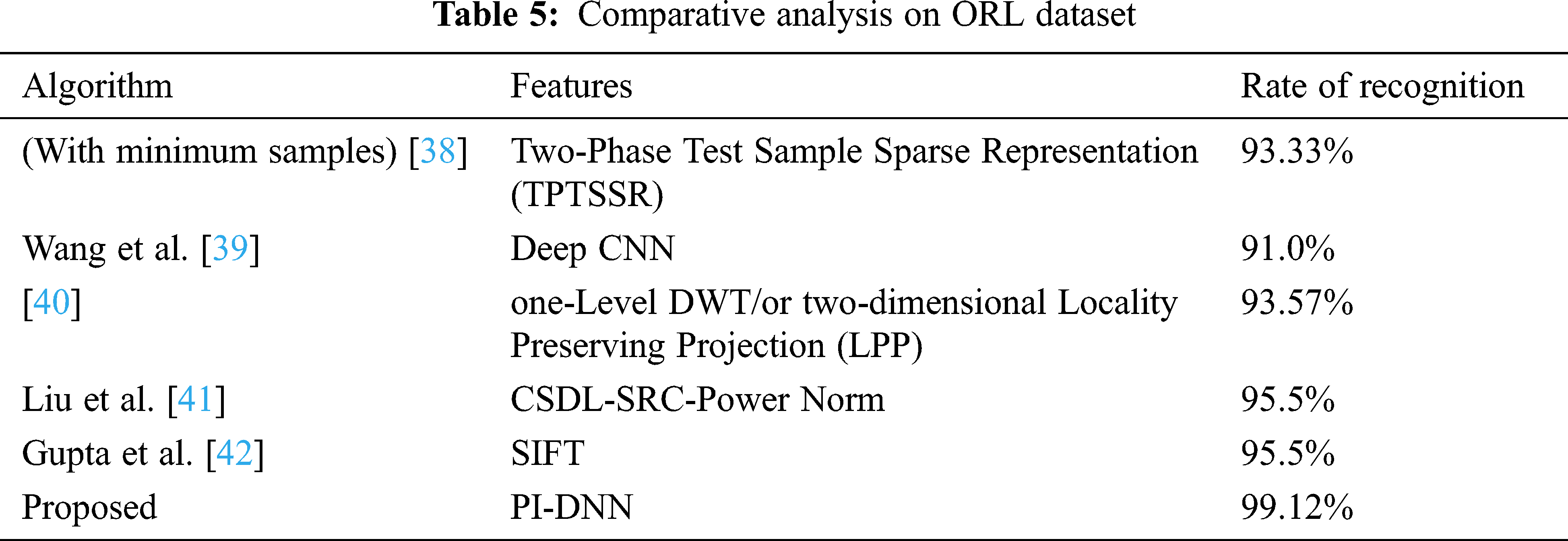
The proposed model has been compared with the several existing approaches on ORL dataset as shown in above table. Higher recognition rate resulted from proposed PI-DNN classifier compared with several techniques on ORL dataset. Due to inefficiency in handling the images occlusion, the existing studies [42] shows not better performances. Assessing the performance of accuracy, precision, recall and F1-score in Deep learning CNN method by testing them on other standard databases and improving the result is considered as the future work.

5  Conclusion

In this research, the novelty in deep neural network for person identification (PI-DNN) has been proposed that gives a high accuracy rate of face recognition by using Local Phase Quantization (LPQ), Geometric-based features and direction graph-based feature extraction methods, and Convolutional Neural Network. This proposed model is used for effective person recognition that is implemented for criminal identification and to evaluate the human faces in crowd taken from LFW and ORL dataset. Various experimental and performance analyses such as classification accuracy, recognition rate, recall, precision, and F1-score performance value of the proposed technique outperforms other existing methods by high efficiency and recognition value ensuring its supremacy over existing methods. This verifies that the proposed approach is more efficient in the feature extraction and more stable, less over fitting the training data or better generalization. The proposed framework performed well with respect to seven considered metrics by showing an outstanding performance than other methods which is confirmed through results. This efficient performance has proved as an effective system for face detection and recognition.

Funding Statement: The authors received no specific funding for this study.

Conflicts of Interest: The authors declare that they have no conflicts of interest to report regarding the present study.

This work is licensed under a Creative Commons Attribution 4.0 International License, which permits unrestricted use, distribution, and reproduction in any medium, provided the original work is properly cited.