Intelligent Automation & Soft Computing DOI:10.32604/iasc.2022.023398
Article

Hyperparameter Tuned Bidirectional Gated Recurrent Neural Network for Weather Forecasting

S. Manikandan1,* and B. Nagaraj2

1Department of Information Technology, Karpagam College of Engineering, Coimbatore, 641032, India
2Principal Rathiniam Technical Campus, Coimbatore, 641021, India
*Corresponding Author: S. Manikandan. Email: manikandanms@kce.ac.in
Received: 06 September 2021; Accepted: 10 November 2021

Abstract: Weather forecasting is primarily related to the prediction of weather conditions that becomes highly important in diverse applications like drought discovery, severe weather forecast, climate monitoring, agriculture, aviation, telecommunication, etc. Data-driven computer modelling with Artificial Neural Networks (ANN) can be used to solve non-linear problems. Presently, Deep Learning (DL) based weather forecasting models can be designed to accomplish reasonable predictive performance. In this aspect, this study presents a Hyper Parameter Tuned Bidirectional Gated Recurrent Neural Network (HPT-BiGRNN) technique for weather forecasting. The HPT-BiGRNN technique aims to utilize the past weather data for training the BiGRNN model and achieve the effective forecasts with minimum time duration. The BiGRNN is an enhanced version of Gated Recurrent Unit (GRU) that follows the process of passing input via forward and backward neural network and the outputs are linked to the identical output layer. The BiGRNN technique includes several hyper-parameters and hence, the hyperparameter optimization process takes place using Bird Mating Optimizer (BMO). The design of BMO algorithm for hyperparameter optimization of the BiGRNN, particularly for weather forecast shows the novelty of the work. The BMO algorithm is used to set hyperparameters such as momentum, learning rate, batch size and weight decay. The experimental result the HPT-BiGRNN approach has resulted in a lower RMSE of 0.173 whereas the Fuzzy-GP, Fuzzy-SC, MLP-ANN and RBF-ANN methods have gained an increased RMSE of 0.218, 0.216, 0.202 and 0.245 respectively.

Keywords: Weather forecast; time series prediction; deep learning; parameter tuning; bigrnn model; metaheuristics

1  Introduction

Weather conditions like wind, temperature and humidity profoundly affects human livelihood. Weather prediction offers analytical support to the smart transportations like air visibility analysis, traffic flow prediction, etc. [1]. As we know, traffic congestions and accidents are highly possible in weather conditions like heavy fog, heavy rain and so on. Timely and accurate weather prediction can save us from weather disasters [2]. Weather prediction represents the scientific method of forecasting the state of atmosphere depending on time and certain locations [3]. Numerical Weather Prediction (NWP) utilizes computer algorithm for prediction based on the present weather condition by resolving a huge system of non-linear arithmetical equations on certain arithmetical model. In recent years, Various NWP methods have been proposed namely Weather Research and Forecasting (WRF) models. Based on [4], data driven computer modelling system could be utilized for reducing the computation power of NWP models. Especially, Artificial Neural Networks (ANN) could be employed for their adaptive nature and learning abilities based on previous knowledge [5]. Such feature makes the ANN technique most attractive in application domain to resolve highly non-linear phenomena.

The Artificial Neural Network (ANN) is one of the robust data modelling tools which can represent and capture complicated relations between outputs and inputs. It is proposed by the inspiration of executing artificial system which can implement intelligent tasks like human brain. Generally, ANN is capable of approximating any non-linear functions [6]. The Deep Neural Network (DNN) is a type of ANN made up of multilayer architectures that can recreate the raw datasets from the original feature space to a learned feature space. In other word, they could “learn” features through Neural Network (NN) rather than choosing features automatically and attain better generalization and higher accuracy through the learned feature. Deep Learning (DL) has accomplished a promising result in several fields like speech recognition, computer vision, scientific fields in physics, chemistry, bio-information and natural linguistic programming [7]. Recently, DL models are used for time sequence problems, where the correlation of the features is apparent, however, it is difficult to determine. Particularly, if the system behaviour is controlled by temporal/spatial contexts (like weather scheme), conventional Machine Learning (ML) methods are not suitable unlike DL methods, that are capable of manually extracting spatial and temporal features for better understanding of the system [8]. When the correlations are analysed and the feature is represented correctly, the prediction performance would be enhanced that is suitable to analyse the features of time sequence. According to this, several researchers have used DL for predicting weather conditions and few traditional complexities in forecasting would be tackled by a data driven method.

As the DL model performs well on weather forecasting problems, this study develops a Hyperparameter Tuned Bidirectional Gated Recurrent Neural Network (HPT-BiGRNN) technique that primarily executes the prediction process using BiGRNN technique. Secondly, the hyperparameters in the BiGRNN technique are optimally adjusted by the BMO algorithm. The design of BMO algorithm based on the mating behaviour of the birds helps to optimally select the hyperparameters of the BiGRNN technique and thereby boosting the overall predictive performance. A wide range of simulation analysis take place on the benchmark dataset and the experimental results are investigated under various aspects.

2  Prior Weather Forecasting Approaches

This section provides an extensive review of weather forecasting approaches available in the literature. Castro et al. [9] proposed a STConvS2S network, a DL framework constructed to learn spatial-temporal data dependency with convolution layer. The presented framework resolves the two main limitations of convolution network for predicting the sequence using the past data such as (1) it requires the length of output and input series to be equivalent and (2) they violate the temporal orders at the time of learning procedure. Sundaram [10] evaluated and developed the short-term weather prediction model with LSTM and calculate the performance of the traditional WRF-NWP models. The presented model consists of stacked LSTM layer which employs surface weather parameters with time period for weather forecasting. These models are tested with distinct numbers of LSTM layer, optimizer and learning rate that are optimized to an efficient short-term weather prediction.

Salman et al. [11] constructed an adaptive and robust statistical model to forecast univariate weather variables at Indonesian airport areas to examine the effects of intermediate weather variables associated with the prediction accuracy through single layer LSTM models and multilayer LSTM models. The presented method is an extension of LSTM models that includes intermediate variable signals to LSTM memory blocks. An approach based on the DNN model [12] for learning higher resolution demonstration from lower resolution prediction of weather as a real time application. The study result shows the outstanding performances and the approach is lightweight enough to run-on moderate computer system.

Rasp et al. [13] proposed a mixed model that uses a subset of original weather trajectory integrated with postprocessing steps of DNN model that represent nonlinear relationship not considered in the present postprocessing/mathematical model. A data driven methods with an efficient data fusion method for learning from the past data that integrates previous knowledge from NWP [14]. They consider the weather forecast problems as an end-to-end DL problem and resolve them by presenting a new NLE loss function. A significant advantage of the presented model is that it concurrently implements uncertainty quantification and single value prediction that represents the DUQ model.

Hewage et al. [15] proposed a lightweight data driven weather prediction models by examining and relating the performance of temporal modelling approach of LSTM and TCN with a dynamic ensemble method, traditional ML approaches, statistical forecasting approaches and the conventional WRF-NWP models. Singh et al. [16] used the UNET framework of DCNN using residual learning to learn global data driven model of precipitation. It is trained over reanalysis datasets proposed on the cubed sphere prediction to minimize error because of its spherical distortions. The result is related to the operational dynamical models by the India Meteorological Departments. The theoretical DL based models show doubling of grid points and area average skills evaluated in Pearson correlation coefficient in relation to operational systems. BiGRNN is a type of artificial neural network that is particularly well suited for evaluating and processing time sequence data. This is in contrast to standard neural networks, which are based on the weight connection between the layers. In order to maintain information from the previous instant, BiGRNN uses hidden layers, and the output is impacted by the present states and memories from the past.

An ensemble predictive scheme with DLWP models [17] that recurrently predict key atmospheric variables using 6 h’ time resolution. These models use CNN on cubed sphere grids for producing global predictions. This method is computational effective, as it requires only 3 min on individual GPU for producing 320 member sets of 6 weeks forecast at 1.4° resolution. Ensemble spread is mainly built by randomizing the CNN training procedure for creating a set of 32 DLWP methods. In Peng et al. [18], a novel NN predictive model named EALSTM-QR has been proposed to predict the wind power considering the input of NWP and the DL methods. In this method, there are four major steps namely Attention, Encoder, bi-LSTM and QR. The combinational input contains the past wind power data and the extracted feature attained from the NWP at Attention and Encoder level. The bi-LSTM is used for generating the wind power time sequence predictive results.

3  The Proposed Weather Forecasting Model

The new BiGRNN technique is designed to effectively estimate the weather conditions. The BiGRNN technique encompasses a two-stage process namely BiGRNN based prediction process and BMO based hyperparameter tuning process. Fig. 1 demonstrates the process of proposed HPT-BiGRNN model.

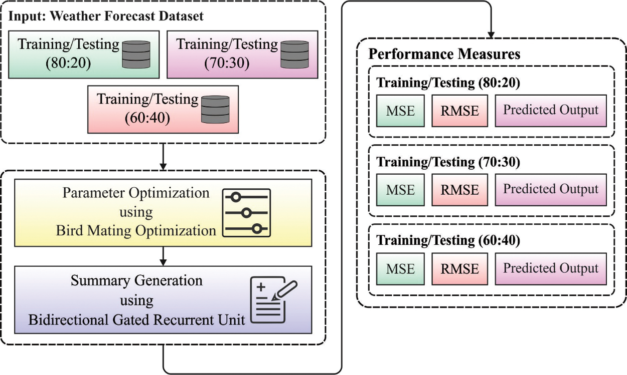
Figure 1: The process of HPT-BiGRNN model

3.1 Weather Forecasting Using BiGRNN Model

At the initial weather forecasting process, the BiGRNN technique receives the previous weather data as input and estimates the future weather condition. The RNNs capability of forecasting its output is well suitable for sequential data. The RNN has a hidden state h, that estimates the input value x and their preceding state. Consider the input series x1, x2, …xn, the RNN is signified by Eq. (1) and Eq. (2) for evaluating the output yt. Here, ht refers to the hidden state at time step t; Whh, Whx and Wyh are the weights of the hidden-to-hidden layer connections, input connections and hidden-to-output connections respectively. bh represents the bias to the hidden state and by implies the bias to the output state. f represents the activation function implemented on the hidden and output nodes throughout the network.

ht=f(Whhht−1+Whxxt+bh)  (1)

yt=f(Wyhht+by) (2)

A major difference between RNNs and GRU is that GRU can capture long term dependencies and address the vanishing gradient issue frequently encountered if trained RNN [19]. During this unit the hidden state ht of GRU is computed as follows.

ht=u⊗h~t+(1−u)⊗ht−1 (3)

where u refers to the update gate that checks whether ht is upgraded or not and ⊗ is an element-wise multiplication. The upgrade gate u is upgraded by implementing the sigmoid logistic function σ and it is given by,

ut=σ(Wuhht−1+Wuxxt+bu) (4)

The candidate cell is updated using the hyperbolic tangent as follows.

h~t=tanh(Whxxt+Whh(r⊗ht−1)+bh)  (5)

where r represents the reset gate for computing the relevance of ht−1 to ht. The reset gate r is estimated in a subsequent manner by,

rt=σ(Wrhht−1+Wrxxt+br) (6)

The BiGRNN has improved 2 layer framework that gives the resultant layer with contextual data of input at all moments. The idea of Bi-GRNN is that the input order is passed by forward NN and backward NN and later, the output of these two are related with similar resultant layer. Fig. 2 shows the framework of Bi-GRU model. During the Bi-GRNN of all layers, the forward layer computes the outcome of hidden layer at every time from forward to backward and the backward layer computes the outcome of hidden layer at every time from backward to forward [20].

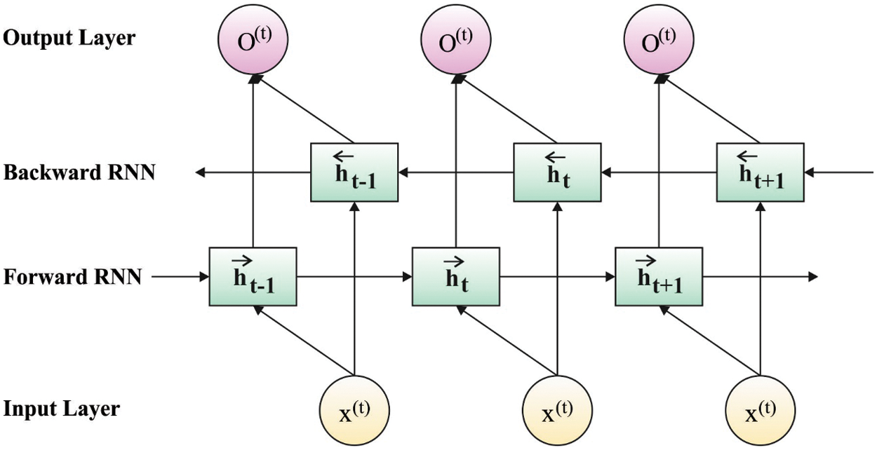
Figure 2: Structure of Bi-GRU model

The resultant layer superimposes and normalizes the output of forward and backward layers at all moments as follows.

ht1→=f(wxh1→xt+wh1→h1→ht−11→+bh1→) (7)

ht1←=f(wxh1←xt+wh1←h1←ht−11←+bh1←) (8)

ht2→=f(wh1→h2→ht1→+wh2→h2→ht−12→+bh2→) (9)

ht2←=f(wh1←h2←ht1←+wh2←h2←ht−12←+bh2←) (10)

yt=g(wh2→yht2→+wh2←yht2←+by) (11)

where ht1→∈RH and ht2→∈RH are the resultant vectors of hidden layers of the forward layer from 1st and 2nd layers of Bi-GRNN at time t, H refers to the number of units from the GRU cells, ht1←∈RH and ht2←∈RH are the resultant vectors of hidden layers of the backward layer from 1st and 2nd layers of the Bi-GRNN at time t, yt ∈ RT is the score of matching word on all labels at time t, T refers to the count of tags, xt signifies the NN input at time t, f demonstrates the GRNN modelling, g refers to the activation functions, where g(x)i=exiΣk=1nexk . w and b represents the weight matrices.

3.2 Hyperparameter Optimization Using BMO Algorithm

The BiGRNN technique has several hyperparameters and the BMO algorithm is used to optimally select the momentum, learning rate, batch size and weight decay. The BMO is a population based stochastic search method developed for addressing continual optimization problem [21]. The behaviour of this algorithm depends on the mating strategy of bird species during mating season. The mating procedure of birds include the usage of three primary operators for producing a novel generation namely mutation, two parents mating and multi parents mating. In Two parents mating, they mate with one another for breeding only one novel breed, while in multi parents mating, a parent mate with at least two other parents for breeding one novel breed. Alternatively, Mutation is a method where the female parents produce novel broods without male parent by changing their own genes. On the traditional BMO algorithm, the assumptions that every bird in the society could modify its own strategy, once a novel generation is upgraded. Always, the birds with maximum fitness value are selected as polyandrous and parthenogenetic, where the birds with poor fitness value are selected as promiscuous. The residual bird in the society is considered as polygynous/monogamous bird. Parthenogenesis is a kind of mating process where the females might generate a brood without mating with males. In this way, all females try to generate their broods by modifying her genes with predetermined rates. All females in the parthenogenetic groups produce a brood as follows.

for i = 1:n

 if r1 > mcfp

  xbrood (i) = x(i) + μ × (r2 − r3) × x(i);

 else

  xbrood (i) = x(i)

 end

end

whereas x(i) represents the ith birds, xbrood indicates the resulting broods, n denotes the dimensional problems (amount of genes), mcfp signifies the mutation control factors of parthenogenesis, r1 denotes the arbitrary values in the range of zero and one, μ denotes the step size. Monogamy is the two parents mating type where a male bird tends to mate with only one female bird. All male birds evaluate the qualities of female birds through a probabilistic method for selecting its mate. Females with good genes have a high possibility of being designated. Eq. (13) illustrate the procedure of generating novel broods from 2 designated parents [22].

x→i=x→+w×r→.×(x→i−x→)

c = a arbitrary value in the range of 1 to  n

if r1 > mcf

   xbrood (c) = l(c) − r2 × (l(c) − u(c));

End

whereas w represents a time differing weights for adjusting the designated female birds, r indicates a 1 × d vector where all the elements are randomly distributed numbers in the range of zero and one also this arbitrary vectors influence the equivalent elements of (x→i−x→),n represnts the dimensional problems, mfc is the mutation control factor lies between zero and one, u & l represents the upper bound and lower bound of the element respectively. From Eq. (13), it is clear that, all males search for a worthy female for producing good quality broods through his genes to generate novel genes. Next, the males try to enhance their generated broods by mutating another broods’ gene with 1 − mcf.

Polygamy is a multiparent mating procedure where males try to generate broods by mating with more than one female bird. The advantage of multi mating procedure is to generate broods with good genes. Naturally, a polygynous bird mate with many female birds producing several broods. After choosing the female birds through the selection process, all males mate with their designated female birds. The resulting broods are generated as follows.

x→i=x→+w×∑j=1n1⁡r→j.×(x→ji−x→)

C = a arbitrary value in the range of 1 to n

if r1 > mcf

  xbrood (c) = l(c) − r × (l(c) − u(c));

End

Let ni be the number of selected females and xji denote the jth selected birds. In BMO, promiscuous birds generate novel broods based on Eq. (13). Polyandry is a multi-parent mating system where females search for mating with several male birds. The female bird performs a selection process for selecting males. Later, all females mate with her designated males. In the BMO, polyandrous birds generate novel broods based on Eq. (14). The process of BMO is given as follows.

Step 1 (Parameter Initiation): Initiate the succeeding BMO parameter

Step 2 (Society Initiation): Arbitrarily initiate a group of possible solutions and include them in society. All the solutions are considered as birds and it is stated by a vector, using n length.

Step 3 (Society Calculation): Evaluate the quality of birds through a calculation process.

Step 4 (Ranking): Sort the birds in the society according to their quality.

Step 5 (Classification): split the society into five clusters of birds namely promiscuous, monogamous, polyandrous, parthenogenetic and polygynous. The polyandrous and parthenogenetic groups are considered as a female bird and the rest of the groups are considered as a male bird. The percentage of all the groups is determined at the parameters’ initiation step.

Step 6 (Breeding): all the birds produce novel broods in their own pattern.

Step 7 (Substitution): When the quality of broods is higher than the quality of birds in the society, the brood replaces the bird or else, the birds remain in the society and the broods are abandoned.

Step 8 (End Criteria): Reiterate the steps 4 to 7 until a predefined NG is carried out.

Step 9 (Report the optimal): choose an optimal quality of birds in the society as an optimal solution. Fig. 3 illustrates the flowchart of BMO technique.

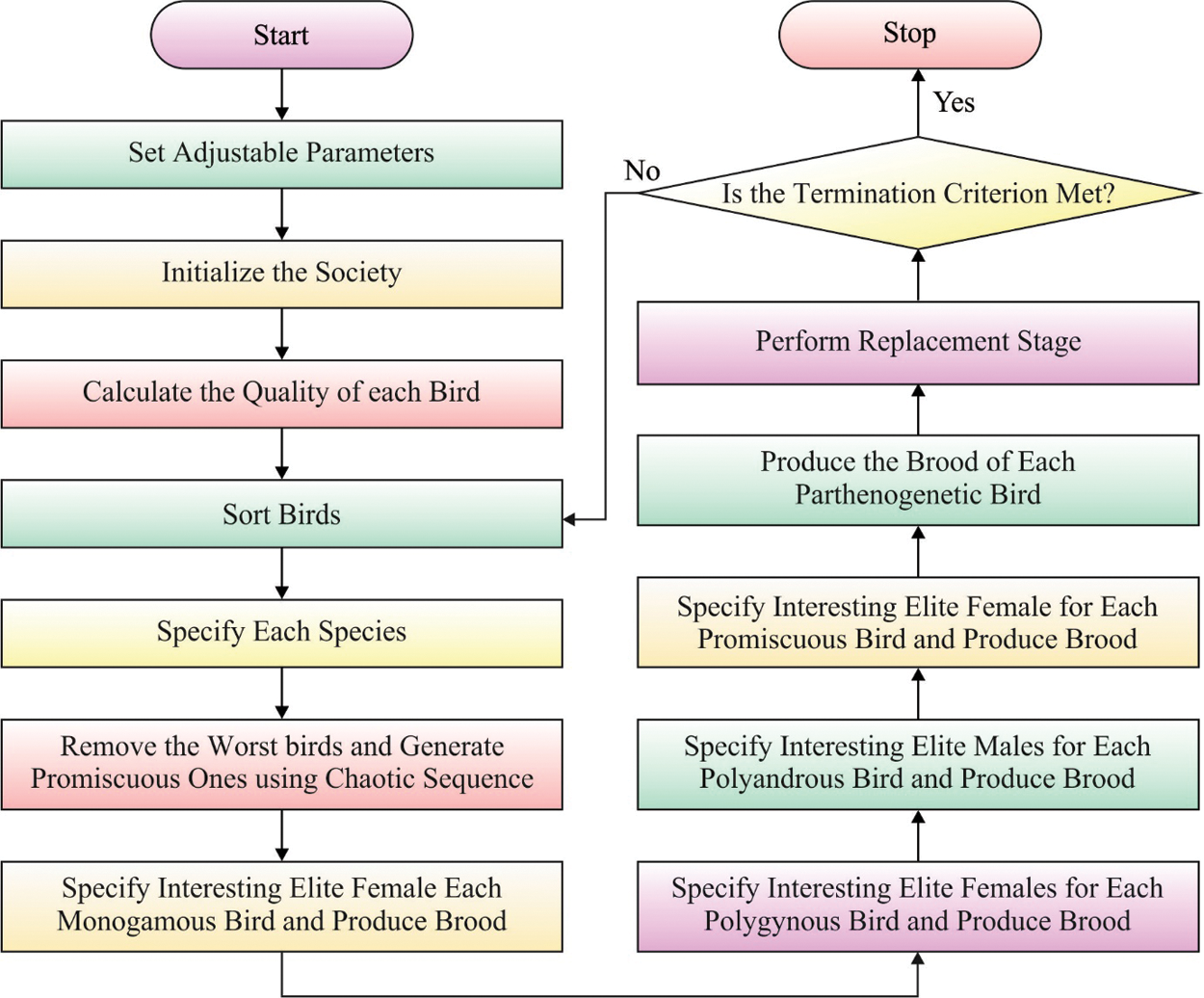
Figure 3: Flowchart of BMO algorithm

4  Performance Validation

This section examines the performance of the HPT-BiGRNN technique on the weather forecasting process. The results are examined under varying sizes of training/testing data. Fig. 4 investigates the forecasting results of the HPT-BiGRNN technique with training/testing data of 80:20 and the results proved that the HPT-BiGRNN technique has attained a predicted value which is highly closer to the actual value. For instance, under 1 h, the HPT-BiGRNN technique has offered a predicted value of 7.6700 whereas the actual value is 7.6400. In addition, under 5 h, the HPT-BiGRNN method has obtained a predicted value of 7.6800 whereas the actual value is 7.6400. Also, under 10 h, the HPT-BiGRNN method has attained a predicted value of 8.8200 whereas the actual value is 8.8600. Additionally, under 15 h, the HPT-BiGRNN approach has offered a predicted value of 9.1600 whereas the actual value is 9.1000. Eventually, under 24 h, the HPT-BiGRNN method has obtained a predicted value of 7.5600 whereas the actual value is 7.5900.

Figure 4: Weather forecast analysis of HPT-BiGRNN model on training/testing data (80:20)

Fig. 5 examines the forecasting outcomes of the HPT-BiGRNN approach under varying training/testing data of 70:30. The results depicted that the HPT-BiGRNN method has obtained a predicted value which is extremely closer to the actual value. For instance, under 1 h, the HPT-BiGRNN method has obtained a predicted value of 7.5600 whereas the actual value is 7.6400. Besides, under 5 h, the HPT-BiGRNN technique has a predicted value of 7.5500 whereas the actual value is 7.6400. In the meantime, under 10 h, the HPT-BiGRNN manner has offered a predicted value of 8.9600 whereas the actual value is 8.8600. Eventually, under 24 h, the HPT-BiGRNN method has offered a predicted value of 7.6600 whereas the actual value is 7.5900.

Figure 5: Weather forecast analysis of HPT-BiGRNN model on training/testing data (70:30)

Fig. 6 explores the forecasting results of the HPT-BiGRNN method under varying training/testing data of 60:40. The outcomes exhibited that the HPT-BiGRNN technique has reached a predicted value that is highly closer to the actual value. For sample, under 1 h, the HPT-BiGRNN technique has obtained a predicted value of 7.7500 whereas the actual value is 7.6400. In line with, under 5 h, the HPT-BiGRNN technique has offered a predicted value of 7.7500 whereas the actual value is 7.6400. Followed by, under 10 h, the HPT-BiGRNN model has offered a predicted value of 9.0200 whereas the actual value is 8.8600. Eventually, under 24 h, the HPT-BiGRNN algorithm has a predicted value of 7.7700 whereas the actual value is 7.5900.

Figure 6: Weather forecast analysis of HPT-BiGRNN model on training/testing data (60:40)

Tab. 1 and Fig. 7 examines the performance of the HPT-BiGRNN technique in terms of MSE under varying training/testing data. The figure shows that the HPT-BiGRNN technique has resulted in effective outcomes with minimal MSE values under varying duration and training/testing data size. For instance, with 1 h, the HPT-BiGRNN technique has attained an MSE of 0.030, 0.080 and 0.110 under the training/testing data of 80:20, 70:30 and 60:40 respectively. Furthermore, with 5 h, the HPT-BiGRNN approach has reached an MSE of 0.040, 0.090 and 0.110 under the training/testing data of 80:20, 70:30 and 60:40 respectively. Then, with 10 h, the HPT-BiGRNN technique has gained an MSE of 0.040, 0.100 and 0.160 under the training/testing data of 80:20, 70:30 and 60:40 respectively. Simultaneously, with 24 h, the HPT-BiGRNN algorithm has obtained an MSE of 0.030, 0.070 and 0.180 under the training/testing data of 80:20, 70:30 and 60:40 respectively.

Figure 7: MSE analysis of HPT-BiGRNN model

Tab. 2 and Fig. 8 validates the performance of the HPT-BiGRNN method with respect to RMSE under varying training/testing data. The figure demonstrated that the HPT-BiGRNN technique has resulted in effective outcomes with the lower RMSE values under varying duration and training/testing data size. For sample, with 1 h, the HPT-BiGRNN algorithm has reached an RMSE of 0.173, 0.283 and 0.332 under the training/testing data of 80:20, 70:30 and 60:40 respectively. Furthermore, with 5 h, the HPT-BiGRNN technique has attained an RMSE of 0.200, 0.300 and 0.331 under the training/testing data of 80:20, 70:30 and 60:40 respectively.

Figure 8: RMSE analysis of HPT-BiGRNN model

Then, with 10 h, the HPT-BiGRNN manner has attained an RMSE of 0.200, 0.316, and 0.400 under the training/testing data of 80:20, 70:30, and 60:40 correspondingly. Afterward, with 20 h, the HPT-BiGRNN technique has achieved an RMSE of 0.224, 0.283, and 0.332 under the training/testing data of 80:20, 70:30, and 60:40 correspondingly. Simultaneously, with 24 h, the HPT-BiGRNN methodology has obtained an RMSE of 0.173, 0.265, and 0.424 under the training/testing data of 80:20, 70:30, and 60:40 correspondingly.

A brief comparative results analysis of the HPT-BiGRNN technique with existing ones interms of RMSE take place in Tab. 3 and Fig. 9 [23]. The comparison study portrayed that the HPT-BiGRNN technique has accomplished proficient results with the least RMSE values. For instance, with 1 h, the HPT-BiGRNN technique has resulted in a lower RMSE of 0.173 whereas the Fuzzy-GP, Fuzzy-SC, MLP-ANN, and RBF-ANN techniques have obtained a higher RMSE of 0.205, 0.225, 0.239, and 0.254. Similarly, with 10 h, the HPT-BiGRNN manner has resulted in a lower RMS of 0.200 whereas the Fuzzy-GP, Fuzzy-SC, MLP-ANN, and RBF-ANN algorithms have obtained an increased RMSE of 0.232, 0.243, 0.255, and 0.297. At the same time, with 15 h, the HPT-BiGRNN technique has resulted in a lesser RMSE of 0.245 whereas the Fuzzy-GP, Fuzzy-SC, MLP-ANN, and RBF-ANN methodologies have achieved a maximal RMSE of 0.251, 0.268, 0.273, and 0.289.

Fig. 9: Comparative analysis of HPT-BiGRNN model with existing techniques

Eventually, with 24 h, the HPT-BiGRNN approach has resulted in a lower RMSE of 0.173 whereas the Fuzzy-GP, Fuzzy-SC, MLP-ANN and RBF-ANN methods have gained an increased RMSE of 0.218, 0.216, 0.202 and 0.245 respectively. It is apparent that the HPT-BiGRNN technique has accomplished the maximum prediction results compared to the existing techniques.

5  Conclusion

In this study, a new BiGRNN technique is designed to effectively predict the weather conditions. The BiGRNN technique encompasses a two-stage process namely BiGRNN based prediction process and BMO based hyperparameter tuning process. Primarily, the past weather data is used by the BiGRNN model to predict the weather condition. Later, the hyperparameters involved in the BiGRNN technique can be optimally tuned by the BMO algorithm. A wide range of simulation analysis take place on the benchmark dataset and its experimental results are investigated under various aspects. The detailed result analysis proves that the BiGRNN technique has outperformed the recent state of art approaches in terms of different measures.The experimental result the HPT-BiGRNN approach has resulted in a lower RMSE of 0.173 whereas the Fuzzy-GP, Fuzzy-SC, MLP-ANN and RBF-ANN methods have gained an increased RMSE of 0.218, 0.216, 0.202 and 0.245 respectively. In future, the BiGRNN technique can be tested using real time data to predict the rainfall and traffic flow.

Funding Statement: The authors received no specific funding for this study.

Conflicts of Interest: The authors declare that they have no conflicts of interest to report regarding the present study.

This work is licensed under a Creative Commons Attribution 4.0 International License, which permits unrestricted use, distribution, and reproduction in any medium, provided the original work is properly cited.