DOI:10.32604/iasc.2022.023079
| Intelligent Automation & Soft Computing DOI:10.32604/iasc.2022.023079 | |
| Article |
Transformer Less Grid Integrated Single Phase PV Inverter Using Prognosticative Control
1Department of Electrical and Electronics Engineering, R.M.K Engineering College, Chennai, 601206, Tamil Nadu, India
2Department of Mechanical Engineering, Dr. M G R Educational and Research Institute, Chennai, 601206, Tamil Nadu, India
*Corresponding Author: Chandla Ellis. Email: chandalaellis234@gmail.com
Received: 27 August 2021; Accepted: 22 October 2021
Abstract: Nature's remarkable and merciful gift to the planet Earth is sunlight which may be highly lucrative if harvested and harnessed properly. Photovoltaic (PV) panels are used to convert the solar energy to electrical energy which are currently used to feed AC loads/grid. In this paper, modelling, performance and power flow studies of grid connected single phase inverter fed from PV array under steady state as well as transient conditions are considered. This paper focuses on the study and development of analytical model of micro-grid integrated single phase five level cascaded H-bridge inverter (MGISPFLCHBPVI) powered by a PV panel. A simple power control strategy for MGISPFLCHBPVI is also considered. The simulations are completely carried out using MATLAB software for power-flow studies. The performance characteristics of the inverter are studied from the analytical model developed. The validation of the analytical model is carried out by comparing the results of simulation in Simulink/Matlab. In order to reduce the time to reach steady state taken by the system, a simple PQ control strategy for insolation is introduced in this paper. The proposed method is evaluated based on performance parameters such as settling time and rising time of the system compared with the results available in the literature.
Keywords: AC loads/grid; PV array; PV panels; single phase inverter; switches; P-Q control; insolation
Sunlight is readily available in abundance all over the world and its proper deployment eliminates approximately 45% power deficiency existing globally. Extracting maximum power from PV array increases the overall efficiency of the PV system [1]. In order to extract maximum energy available from PV array, power electronic converters are designed and utilized with solar arrays and load thus the system serves as a stand-alone PV system [2]. Solar cells are the basic unit of PV generator, which are connected in series to build a PV module. PV strings are built by connecting solar modules in series. The PV strings are connected together in series and parallel to build a PV array to meet the voltage and power requirements [3].
The energy yield study of 1kWp residential PV plant at Chennai is considered for brief discussion. The diurnal, monthly and seasonal variation of solar radiation at Chennai during the years 2013, 2014 and 2015 are recorded. Similarly, the output energy yield of the PV plant during the year 2013, 2014 and 2015 are also estimated and recorded [4]. The research based on the I-V and P-V performance characteristics of PV system for varying environmental conditions is considered in [5]. Solar array is designed and its system performances are validated under varying environmental and load conditions [6]. Different models of panel such as four and five parameters are briefly discussed and it is inferred that the performance of five parameter model matches closely with the manufacturers data as discussed in [7–9]. A PV panel cannot be directly integrated to unipolar/bipolar dc bus and it requires a suitable dc-dc converter as explained in [10]. The single phase inverter is required in order to transport power from PV array to AC micro-grid. Different switching pulse generation methods and configurations for single phase grid connected inverter are studied and compared as presented in [11]. Further, it is mentioned that the system takes much time to reach steady state values. Different power control techniques involving closed loop methods for grid integrated PV inverter are briefly discussed in [12–16].
Based on the review, a modified five parameter analytical model of PV array is developed and its performance is obtained for different operating conditions. This paper focuses on the study and development of analytical model of micro-grid integrated single phase five level cascaded H-bridge inverter (MGISPFLCHBPVI) powered by a PV panel as shown in Fig. 1. A simple power control strategy for MGISPFLCHBPVI is also considered. The simulations are completely carried out using MATLAB software for power-flow studies.

Figure 1: Circuit model of MGISPFLCHBPVI
The equivalent electrical circuit model of a silicon photovoltaic cell consists of a controlled dc current source (IL), a PN junction diode D, a shunt resistance Rsh connected in parallel and a series resistance Rse as shown in Fig. 2.

Figure 2: Single diode model of a solar cell
The mathematical expression used to calculate the output current of solar cell is given by Eq. (1).
where IL is the measured photocurrent for the irradiance S(W/m2), I0 is the diode reverse saturation current, VT is diode thermal voltage and VT = kb*Tcell/q, kb is Boltzmann constant and kb = 1.3807 × 10 −23 J K−1, q is charge of a proton where q = 1.602 × 10⁻¹⁹ C, Tcell is working temperature of PV cell, VPV is the output voltage across the solar cell, IPV is the output current of the cell, Rse and Rsh are series and shunt resistances, N is diode ideality factor. The ideality factor varies for amorphous cells, and is typically 1–2 for polycrystalline cells and less than 1 for mono-crystalline silicon cells (c-Si). The expression used to calculate the reference and generated photo current are given by Eqs. (2) and (3) respectively.
where IL is the photo-current generated, Sref is standard insolation (1000 W/m2), Iscref is short circuit of PV array at STC, αisc is temperature coefficient of current (0.102%°C−1), Tcell and Tref (298 K or 25°C) are cell and reference temperatures in kelvin.
The expression used to calculate the energy band gap can be written as
where dEgdT is energy band gap coefficient and dEgdT = −0.02677% (eV°C−1), Egref is reference energy band gap of Si diode and it is equal to 1.12 eV.
The diode quality factor and PV array shunt resistance can be mathematically estimated using Eqs. (5) and (6) respectively.
where VMPP and IMPP are peak voltage and peak current of PV array, Rsh(0) is shunt resistance at short circuit condition which can be estimated using Eq. (7).
The mathematical expression used to calculate the reference thermal voltage, array thermal voltage, reference diode reverse saturation current and diode reverse saturation current are given in Eqs. (8)–(11) respectively.
where Iscref and Vocref are short circuit current and open circuit voltage of PV array at standard test conditions(1 kW/m2 at 25°C). Based on Eqs. (1) to (11), the five-parameter mathematical model to calculate PV output current is developed as shown in Fig. 3.

Figure 3: Five-Parameter mathematical model of PV current generator
2.1 Study of Residential PV Plant
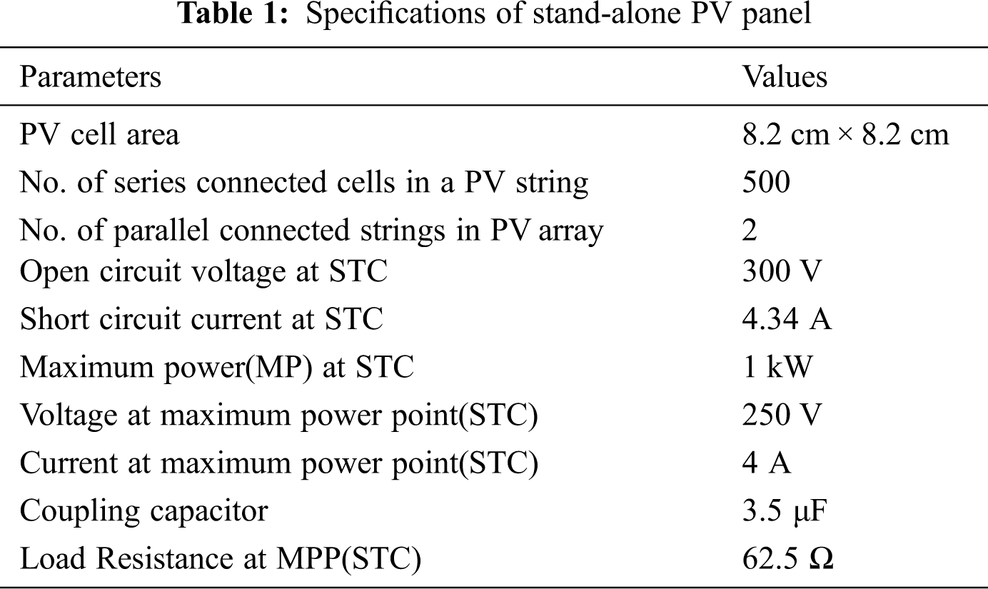
The design and analysis of a 1 kWp, 250 V domestic roof-top PV panel situated at Chennai is considered for performance study. The specification of stand-alone PV panel is shown in Tab. 1.
2.2 Simulink Model of PV System
The Simulink model of stand-alone 1 kW, 250 V PV panel is developed as shown in Fig. 4.

Figure 4: Simulink diagram of stand-alone PV system connected to a resistive load
In a typical scenario both temperature and insolation may vary during an operation. The typical variations of insolation and temperature are depicted in the Figs. 5 and 6 respectively.

Figure 5: Step change in insolation from 850 to 1000 W/m2 at 2 ms

Figure 6: Step change in temperature from 25°C to 40°C at 4 ms
The simulation is run for 6 ms with above data as inputs. The performance of the output voltage for R and RL load are recorded as shown in the Fig. 7.

Figure 7: Load voltage response for temperature and insolation variation
For step increase in insolation from 850 to 1000 W/m2, the output voltage rises exponentially from 222.8 V and settles at 250 V in 0.5 ms. For step increase in temperature from 25 to 40°C, the load voltage exponentially decays from 250 V and settles to 241.3 V in 0.3 ms with an undershoot of about 1 V. The response is in line with the reports published already.
3 Single Phase Five Level Cascaded H-Bridge Inverter
The power circuit of a 1 kW, 230 V, 5.4 A single phase five level cascaded H-bridge inverter (SPFLCHBI) consists of a pair of DC voltage source (VDC), two cascaded H-bridge inverters with eight switches, low pass filter and a load as shown in Fig. 8.

Figure 8: Schematic diagram of SPFLCHBI feeding a load
A pair of 208 V DC is considered as input voltage for SPFLCHBI. The frequency operation of inverter ranges from 49.5 to 50.5 Hz with nominal frequency of 50 Hz. The modulation index ranges from 0.7 to 0.9 with nominal value of 0.8. A 300 V NPN MOSFET is considered for power switch. An LC filter with a cut off frequency of 1.5 kHz is considered for filter operation so that voltage is sinusoidal at the point of coupling to the grid. The filter inductance and filter capacitance are specified as 4 mH and 3 μF respectively. The 1 kW, 230 V resistive loads is realized using a 53 Ω wire wound resistor. In order to realize 1 kW, 230 V inductive load of 0.8 pf, a resistance of 42.32 ohm is connected in series with a 0.1013 H inductor, rated 8 amperes. A 100 μF, 400 V AC capacitor is connected with 42.32 ohm in order to realize a 1 kW, 230 V 0.8 pf capacitive load. The positive and negative half-cycle switching pattern for SPFLCHBI is shown in Tab. 2. The triggering pulse generation using in phase disposition method is shown in Fig. 9.
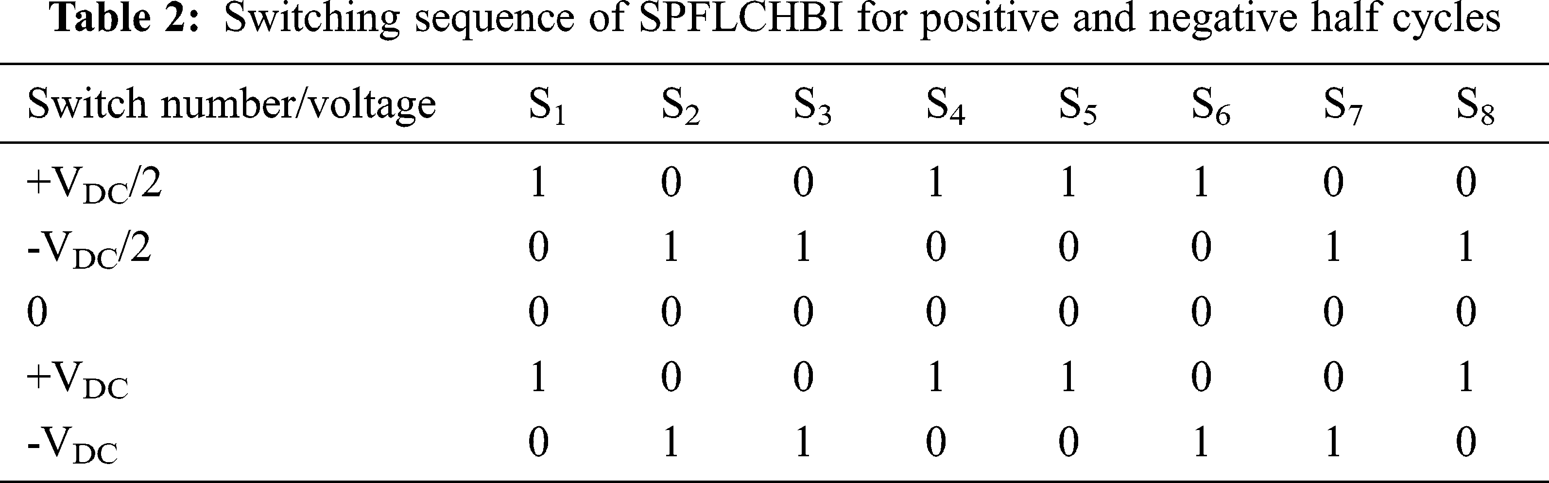

Figure 9: Circuit for gate pulse generation
The carrier signal and modulating signal frequencies are set as 10 kHz and 50 Hz respectively. The modulating and carrier signals waveforms for SPWM is shown in Fig. 10. The switching pulse waveforms for upper and lower bridge switches during one cycle are shown in Figs. 11 and 12 respectively.

Figure 10: Waveforms of modulating and carrier signals for SPWM

Figure 11: Gate pulse waveforms of upper bridge switches during a cycle. (a) Switch S1 (b) Switch S3 (c) Switch S5 (d) Switch S7

Figure 12: Gate pulse waveforms of lower bridge switches during a cycle. (a) Switch S2 (b) Switch S4 (c) Switch S6 (d) Switch S8
The Modulation Index (MI) can be calculated using the expression given in Eq. (12)
where Bm is the amplitude of sinusoidal modulating signal, Bc is the amplitude of triangular carrier signal and n represents the number of CHBI levels.
The RMS voltage for different values of modulation index (MI) under various power factor conditions are calculated and plotted as shown in Fig. 13. For a given MI range 0.7–0.9, VRC > VR > VRL and the variation of RMS voltage with respect to MI is found to be linear. For MI 0.786, the voltage regulation characteristics for different power factors are plotted as shown in Fig. 14. The no-load voltage is set to 231 V. It is observed that when the inverter gets loaded, VRand VRL droops linearly whereas VRC rises almost linear. The voltage regulation of the inverter feeding lagging, leading and unity power factor loads are computed as + 4.35%, −1.37% and + 2.1% respectively.

Figure 13: Steady state RMS output voltage vs. MI for different loads

Figure 14: Regulation characteristics of SPFLCHBI feeding different loads
The Simulink model of 1 kWp stand-alone single phase inverter fed from PV array is developed as shown in Fig. 15. The load resistance is set to 160 Ω to realize 1 kW output. In order to study transient voltage performance of the system, the typical variation in insolation and temperature are considered as shown in Fig. 16. The simulation is run for 80 ms and PV voltage, inverter voltage and inverter current are shown in Figs. 17–19 respectively.

Figure 15: Simulink model of stand-alone single phase inverter fed from PV array

Figure 16: Insolation and temperature variation. (a) Insolation variation (b) Temperature variation

Figure 17: Output voltage response of PV panels

Figure 18: Output voltage waveform

Figure 19: Output current waveform
For step decrease in insolation from 1000 to 800 W/m2 at 0.04 s, the peak voltage decreases from 565.6 V and settles at 553.5 V. The output current peak decreases from 3.535 to 3.46 A. For step increase in temperature from 25°C to 45°C at 0.06 s, the peak voltage decreases from 553.5 V and settles at 520 V. Similarly, the output current peak decreases from 3.46 to 3.21 A. It is seen from the results that there are no noticeable transients in the voltage and current wave forms.
4 Grid Integrated Single Phase Inverter Fed from PV Panels
The analytical model of MGISPFLCHBPVI is developed using MATLAB function as shown in Fig. 20. While integrating the single phase PV inverter system with the grid, the maximum power transmission control is established by implementing a feed forward control strategy such that it eliminates the requirement conventional feedback systems. The modified maximum power point tracking (MPPT) technique is briefly discussed in Section 5.2.

Figure 20: Analytical model of MGISPFLCHBPVI
Based on I-V and P-V characteristics of 1 kWp, 250 V PV array, a 2-D lookup table model for extracting maximum power from PV array is constructed using MATLAB/Simulink platform. Two lookup tables are constructed for estimating VMPP and PMPP with each table having inputs as solar insolation (W/m2) and cell temperature (°C).
The real power (Pg) and reactive power (Qg) injected by inverter to the grid are given by Eqs. (13) and (14) respectively.
where E and V are inverter and grid RMS voltages.
Zg is grid impedance.
δ is angle between E and V (in radians). δ is positive if E leads V and δ is considered negative if E lags V.
In order to operate the inverter in generating region, P > 0 and δ must be positive, i.e., E should lead V by + δ(rad). With grid voltage as reference, the grid current, Ig can be written as
where θ is phase angle between V and Ig.
The necessary real power to be injected into the grid is given by the power tracked from PV array (as discussed in previous sections) at a particular insolation and cell temperature. Thus a dependent PQ control strategy is implemented by estimating modulation index and phase angle of the inverter modulating signal. The mathematical relationship between modulation index and inverter voltage is given in the Eq. (16).
The reference phase angle (δref) and modulation index (mref) are determined using Eqs. (17) and (18) respectively.
where VDC is input voltage of the single phase PV inverter.
Pg_ref and Qg_ref are reference real and reactive powers respectively.
Based on the above Eqs. (13) to (18), a PQ control algorithm is written in m-code format and simulated in MATLAB function block set.
This section focuses on the comparison of P&O method with proposed PQ control strategy developed to inject Pmax from PV panel into the grid. The parameters such as settling time and rising time are used for comparison among various methodologies.
A P&O for MPPT from PV array mentioned in above sections considered for comparison. The PV voltage, current and power responses for variation in insolation and temperature are reproduced as given in this section and these are shown in Fig. 21. It is observed in the figure that the time taken to track peak power from PV array is about 0.58 s.

Figure 21: Transient waveforms of (a) PV voltage (b) PV current (c) PV power
5.2 Performance with Proposed P-Q Control Strategy
The proposed PQ control technique is implemented and the steady state inverter voltage, grid voltage and current waveforms for a period of 3 cycles are obtained at STC as shown in Fig. 22.

Figure 22: Steady state grid voltage, grid current and inverter voltage waveforms at STC
To study the transient voltage response of the grid connected single phase PV inverter system, the typical variations of solar insolation and temperature are considered as already shown in Fig. 20. The panel power and voltage waveforms are shown in Fig. 23. The inverter voltage and grid current and voltage waveforms are captured and are shown in Figs. 24 and 25 respectively.

Figure 23: Panel peak power and peak voltage waveform

Figure 24: Inverter voltage and grid voltage waveform

Figure 25: Grid current and grid voltage waveform
From the Fig. 23, it is observed that the peak power changes from 500 to 248 W whenever there is a change in insolation from 1000 to 500 W/m2 at 40 ms similarly the peak power point voltage changes from 250 to 247.2 V. For step change in temperature from 25°C to 40°C at 80 ms, the peak power of each panel changes from 248 to 233 W. Similarly the peak power point voltage changes from 247.2 to 221.2 V.
From Fig. 22, it is observed that the output voltage waveform reaches steady state within a period of 10 ms whenever there is a step change in insolation or temperature. The efficiency of grid integrated PV inverter system for different insolation conditions is plotted as shown in Fig. 26. The efficiency is defined as the ratio of grid input power to PV output power.

Figure 26: Inverter efficiency for different insolation
The parameters such as settling time and rise time are compared for different technologies are shown in Tab. 3.

It is clear from the table that the settling time taken by the conventional method is large when compared with that of the time taken by proposed control strategy. The rising time is at a minimal microseconds in comparision with other strategy. It is anticipated that the employed method can track the global arrays when evaluating the power yield from the arrays. The estimated power yield from each array is calculated by multiplying the total power retrieved from the two arrays by the stated or estimated respective methods. Fig. 27 shows the estimated power yields from the proposed design, P&O, and GA INC for the aforementioned parameters.

Figure 27: Graphical representation of input power for the grid under various conditions
A 1 kWp PV array fed single phase grid connected inverter system is designed, modeled and simulated for performance study. Analytical models for PV panel and 1-phase inverter were developed. The performance of this model is validated by comparing its results with those obtained from Simulink model. The transient response of the system has been studied by varying insolation and temperature. The proposed PQ control strategy is able to inject the maximum extracted power from PV panel effectively into the grid. Its performance is compared with the conventional methods during transient and steady state periods. It is finally concluded that the settling time was effectively reduced to 10 ms with minimum oscillations in the output voltage waveforms and the proposed methodology results 97.2% efficiency.
Acknowledgement: The authors with a deep sense of gratitude would thank the supervisor for his guidance and constant support rendered during this research.
Funding Statement: The authors received no specific funding for this study.
Conflicts of Interest: The authors declare that they have no conflicts of interest to report regarding the present study.
1. S. Dutta, D. Debnath and K. Chatterjee, “A Grid-connected single-phase transformer less inverter controlling two solar PV arrays operating under different atmospheric conditions,” IEEE Transactions on Industrial Electronics, vol. 65, no. 1, pp. 374–385, 2017. [Google Scholar]
2. M. G. Villalva, J. R. Gazoli and E. R. Filho, “Comprehensive approach to modeling and simulation of photovoltaic arrays,” IEEE Transactions on Power Electronics, vol. 24, no. 5, pp. 1198–1208, 2009. [Google Scholar]
3. Y. Zhang, S. Lyden, B. L. Barra and M. Haque, “A genetic algorithm approach to parameter estimation for PV modules,” in Proc. Power and Energy Society General Meeting, IEEE, Boston, MA, USA, pp. 1–5, 2016. [Google Scholar]
4. M. Alqarni and M. K. Darwish, “Maximum power point tracking for photovoltaic system: modified perturb and observe algorithm,” in Proc. Universities Power Engineering Conf., IEEE, London, UK, pp. 1–4, 2012. [Google Scholar]
5. A. Elbaset, H. Ali and A. E. Sattar, “A modified perturb and observe algorithm for maximum power point tracking of photovoltaic system using buck-boost converter,” Journal of Engineering Sciences, vol. 43, no. 3, pp. 344–362, 2015. [Google Scholar]
6. R. I. Putri, S. Wibowo and M. Rifa, “Maximum power point tracking for photovoltaic using incremental conductance method,” Energy Procedia, vol. 68, pp. 22–30, 2015. [Google Scholar]
7. P. U. Mankar and R. M. Moharil, “Comparative analysis of the perturb and observe and incremental conductance MPPT methods,” International Journal of Research in Engineering and Applied Sciences, vol. 2, no. 2, pp. 60–66, 2014. [Google Scholar]
8. A. M. Zaki, S. I. Amer and M. Mostafa, “Maximum power point tracking for PV system using advanced neural networks technique,” International Journal of Emerging Technology and Advanced Engineering, vol. 2, no. 12, pp. 58–63, 2012. [Google Scholar]
9. S. Messalti, “A new neural networks MPPT controller for PV systems,” in Proc. Int. Renewable Energy Congress, IEEE, Sousse, Tunisia, pp. 1–6, 2015. [Google Scholar]
10. A. E. Khateb, N. A. Rahim and J. Selvaraj, “Optimized PID controller for both single phase inverter and MPPT SEPIC DC/DC converter of PV module,” in Proc. Int. Electrical Machines and Drives Conf., IEEE, Niagara Falls, ON, Canada, pp. 1036–1041, 2011. [Google Scholar]
11. R. Blange, C. Mahanta and A. K. Gogoi, “MPPT of solar photovoltaic cell using perturb and observe and fuzzy logic controller algorithm for buck-boost DC-DC converter,” in Proc. Int. Conf. on Energy, Power and Environment, IEEE, Shillong, India, pp. 1–5, 2015. [Google Scholar]
12. T. N. Nguyen and A. Luo, “Multifunction converter based on lyapunov function used in a photovoltaic system,” Turkish Journal of Electrical Engineering & Computer Sciences, vol. 22, no. 4, pp. 893–908, 2014. [Google Scholar]
13. U. Yilmaz, A. Kircay and S. Borekci, “PV system fuzzy logic MPPT method and PI control as a charge controller,” Renewable and Sustainable Energy Reviews, vol. 81, pp. 994–1001, 2018. [Google Scholar]
14. G. Prathiba, M. Santhi and A. Ahilan, “Design and implementation of reliable flash ADC for microwave applications,” Microelectronics Reliability, vol. 88, pp. 91–97, 2018. [Google Scholar]
15. K. Kalaiselvi and A. Kumar, “Effect of variations in the population size and generations of genetic algorithms in cryptography-an empirical study,” Indian Journal of Science and Technology, vol. 10, no. 19, pp. 1–6, 2017. [Google Scholar]
16. A. Appathurai and P. Deepa, “Design for reliablity: A novel counter matrix code for FPGA based quality applications,” in Proc. Asia Symp. on Quality Electronic Design, IEEE, Kula Lumpur, Malaysia, pp. 56–61, 2015. [Google Scholar]
 | This work is licensed under a Creative Commons Attribution 4.0 International License, which permits unrestricted use, distribution, and reproduction in any medium, provided the original work is properly cited. |