Intelligent Automation & Soft Computing DOI:10.32604/iasc.2022.024252
Article

The Intelligent Trajectory Optimization of Multistage Rocket with Gauss Pseudo-Spectral Method

Lihua Zhu1,*, Yu Wang1, Zhiqiang Wu1 and Cheire Cheng2

1School of Mechanical Engineering, Nanjing University of Science and Technology, Nanjing, 210094, China
2Department of Electrical and Electronic Engineering, Colorado State University, Colorado, United States
*Corresponding Author: Lihua Zhu. Email: zhulihua@njust.edu.cn
Received: 11 October 2021; Accepted: 23 November 2021

Abstract: The rapid developments of artificial intelligence in the last decade are influencing aerospace engineering to a great extent and research in this context is proliferating. In this paper, the trajectory optimization of a three-stage launch vehicle in the powering phase subject to the sun-synchronous orbit is considered. To solve the optimal control problem, the Gauss pseudo-spectral method (GPM) is used to transform the optimization model to a nonlinear programming (NLP) problem and sequential quadratic programming is applied to find the optimal solution. However, the sensitivity of the initial guess may cost the solver significant time to do the Newton iteration or even lead to the local minimum. Aiming at this issue, a good initial guess generated by combination of harmony search and GPM is introduced to help the optimizer to faster and better solve the sun-synchronous orbit (SSO) trajectory optimization. Comparative simulation tests are conducted with the proposed algorithm and popular approaches, the results indicate that with the optimized initial guess, the proposed method could achieve better performance in terms of convergence ability and convergence rate.

Keywords: Trajectory optimization; sun-synchronous orbit; gauss pseudo-spectral method; harmony search; initial guess optimization

1  Introduction

The impact of artificial intelligence (AI) technology on our modern world is now more apparent than ever. The space sector is catching up to these developments, as more and more works are published that incorporate concepts related to AI. Applications of interest range from preliminary spacecraft design to mission operations, from guidance and control algorithms over navigation to the trajectory design and optimization of launch vehicles to only name a few. The SSO mission, as one of the most commonly used forms for space missions, is typically a near-circular low-Earth orbit with an altitude less than 1500 km. The list of past, present, and future Earth orbiting sun-synchronous missions is long and impressive. Classic examples of the SSO missions, such as the ESSA [1], JPSS [2], FY-1 [3], METOR, METOP [4] and others were for weather studies. More recent earth science missions based on SSO are CZ-6, RADARSAT [5] and TERRA [6]. And even now there are several future missions either under development or awaiting launch that will also utilize the SSO within the coming years [7–9]. Given the widespread use of the SSO, it is worthwhile to describe the process of how one goes about selecting the system parameters that define the SSO mission design.

For SSO mission rockets, it is necessary to generate an optimal standard trajectory in advance to complete the binding of shooting elements. Since most satellites comanifest with a larger payload, leaving their launch schedule and trajectory at the mercy of the major payload, the optimal ascending trajectory leading to determination of the maximum payload mass in the desired orbit has been studied. Trajectory optimization problems are generally nonlinear, with optimal control problems with state and control constraints. Numerical methods for solving optimal control problems are generally classified into two major kinds, namely the indirect method and direct method [10]. The indirect method derives the first-order necessary conditions based on the Pontryagin principle of minimum value, converts the optimal control problem into a Hamilton boundary value problem, and then turns to numerical algorithms for solution. The direct method does not need to regain the necessary conditions for optimality, it transforms the optimal control problem into a NLP problem through parameterization, and then obtains the optimal solution through the numerical conversion of the NLP problem [11]. As the fast and maneuverable launch is increasingly important in the development of modern combat, the fast binding of shooting elements is required to save launch preparation time [12–14]. Among the various algorithms, the high computational efficiency of Gauss pseudo-spectral method can meet this challenge, and its application has attracted much attention [15–17] such as the space station attitude control [18], spacecraft orbit transfer under small thrust [19], lunar soft landing trajectory optimization [20], launch vehicle trajectory optimization [21–23], etc.

The pseudo-spectral method uses global interpolation polynomials to approximate the state variables and control variables at a series of discrete points, and transforms the differential equation constraints into algebraic constraints by introducing a pseudo-spectral difference matrix similar to a finite difference matrix. Since the collocation point of the pseudo-spectral method is generally the root of an orthogonal polynomial, it is also called the orthogonal collocation method. Along with the technique improvement, Gauss-Legendre collocation [24], Legendre-Gauss-Radau collocation [25] and hp-adaptive mesh refinement [26] have been developed to enrich it capability. And thanks to the toolbox like GPOPS, PSOPT and DIECOL, the Gauss pseudo-spectral method is able to applied by simply interpolating the boundary conditions provided by the users. However, it is impossible to build a model that is completely consistent with the practice, so that the initial guess value set by the users usually hardly satisfy the dynamic model and path constraints because of the lack of physical knowledge. That is to say, the NLP solver would start at unreasonable points where some constraints can hardly be satisfied, and lead to increased number of Newton iteration [27,28].

Given this issue, this paper contributes to propose a fusion algorithm that employs the harmony search (HS) in Gauss pseudo-spectral framework to generate a good initial value for the subsequent gradient optimization solver. In this paper, the optimization model is firstly established with the maximum remaining mass at the shutdown point, taking into account of the constraints of the dynamic pressure, downrange, and angle of attack. And the sequences that best fit the mission requirements are resolved based on the proposed algorithm. And comparative simulation tests are carried out to demonstrate the effectiveness of our study.

The remainder of the paper is as follows: Section 2 presents the aerodynamic model of the launch vehicle and optimization model. Section 3 describes the method and process of solving the SSO trajectory problem. In Section 4, simulation tests are carried out to demonstrated the effectiveness of the proposed algorithm through a series of comparison. Section 5 concludes the paper.

2  Problem Description

2.1 Launch Vehicle Modeling

A three-stage rocket that is being considered as the launcher, which is a rocket designed to place satellites in sun-synchronous orbit. The description of the structural, propulsive, aerodynamic characteristics and the trajectory model are given as follows.

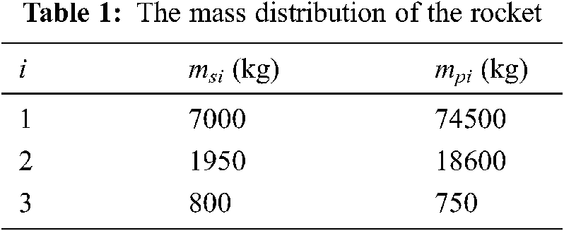
(1)   Mass distribution

To simplify the analysis at hand, the mass distribution of the rocket is depicted in the structural mass and propellant mass of each separate stage. M0 is the initial mass, it is composed of the total mass of all three stages. Thus, we have:

M0=m1+m2+m3 (1)

where, m1, m2 and m3 are the total mass of the three stages, each of them is composed of structural mass msi and propellant mass mpi. The mass distribution for the rocket is shown in the Tab. 1. The initial mass M0 is 102946 (kg).

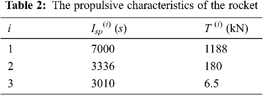
(2)   Propulsive thrust

The propulsion system produces the required thrust to overcome the drag forces and gravity, to lift the launch vehicle from the ground and send it into the designed orbit. And the propulsive characteristic of the launch vehicle can be depicted in terms of thrust magnitude and specific impulse Isp, and the average thrust T and specific impulse Isp of each stage are listed in Tab. 2.

(3)   Aerodynamic model

Aerodynamic forces arise as a result of the relative motion between the launch vehicle and the surrounding air. It can actually be broken down into three components, namely the lift, the drag and the side force. The lift force acts perpendicular to the direction of motion, the drag force is opposite of the motion direction, while the side force is mutually perpendicular to the plane where the lift and the drag lie in. As a valid assumption in the early design, only the drag force is considered in this paper. The expression for the drag force D is:

D=−12ρSmCDv2 (2)

where ρ is the atmospheric density, Sm is the aerodynamic surface area, CD is the drag coefficient and v is the relative speed.

(4)   Trajectory model

The complete description of a launch vehicle’s motion consists of three translational and three rotational degrees of freedom. Since the trajectory of the mass center of the vehicle is more concerned than its attitude motion in the early stage of design. Therefore, in this study, launch vehicle dynamics were modeled using three-degrees-of-freedom equations of motion and standard models of gravity and atmosphere were implemented in the trajectory optimization problem.

r˙(t)=v˙(t)v˙(t)=−μ||r(t)||r(t)+T(t)m(t)u(t)+D(t)m(t) (3)

The two equations in Eq. (4) denotes the kinematic equation that describes the time rate of change of the vehicle’s position and the dynamic equation that describes the vehicle motion under the external forces, respectively. The forces acting on the launch vehicle during powered atmospheric stage are gravity, aerodynamic force and propulsive force.

2.2 Optimization Modelling

In this paper, the maximum payload is set as the optimization purpose to determine the thrust direction subject to the dynamic constraints, path constraints, event constraints and boundaries.

(1)   The objective function is to regulate the control vector to maximize the mass at the end of the last phase.

J=−m(3)(tf) (4)

(2)   The initial settlings are the position and velocity coordinates in the beginning of the mission, which are defined as:

{r(t0)=[5044.5,0.0,3903.0]kmV(t0)=[0.0,0.3679,0.0]km/s (5)

(3)   Event constraints. The terminal constraints are applied to the endpoint of the last phase, which is corresponding to the target sun-synchronous orbit are

{af=7237 kmef=0if=98.8∘ (6)

(4)   The dynamic constraints are a set of ordinary differential equations in state-space form, which utilizes the three-degree-of-freedom motion equations modeled in earth centered inertial frame.

(5)   The path constraints are generally equality or inequality, which are defined for restricting the values’ range in the form of separate or combined functions of the state and/or control variables. In this paper, the thrust direction u is constrained to a unit vector, that is, we take the thrust direction as the optimal control.

|u|=1 (7)

As one of the critical load conditions for the launch vehicle, the dynamic pressure q acts on the outer surface of the vehicle is an important consideration of the structural loads. In our case, the maximum allowable dynamic pressure of the first stage is defined as:

q__phase1≤60kPa (8)

In order to avoid unrealistic trajectories regarding the structural loads, the maximum angle of attack α of the first stage has to be constrained:

−3∘≤α__phase1≤3∘ (9)

In this paper, we also take consideration of the scatter degree of the structural jettisons, so that the downrange of the first stage is constrained as:

800km≤downrange__phase1≤820 km (10)

3  Trajectory Optimization Problem

To solve the SSO trajectory optimization problem, the Gauss pseudo-spectral method is used to transform the optimal control problem to a NLP problem. Although the number of variables and constraints for the original optimal control problem in this paper is not very large, the obtained NLP problem after discretization has large scale and high complexity. In order to quickly find the resolution that satisfies the dynamic constraints, path constraints and terminal constraints, an efficient and accurate optimization algorithm is needed. The commonly used optimization algorithms can be divided into gradient optimization algorithm and intelligent optimization algorithm. Both kinds of the algorithms have their strengths. In this paper, a serial optimization strategy combining harmony search (HS) algorithm with sequential quadratic programming (SQP) algorithm is adopted to do the optimization. The flowchart of the employed optimization resolve is show in Fig. 1. The principle of Gauss pseudo-spectral method is presented in Section 3.1, the harmony search process is introduced in Section 3.2. As SQP algorithm has been very mature so far, and the specific process of the algorithm is complicated, it is not described in this paper.

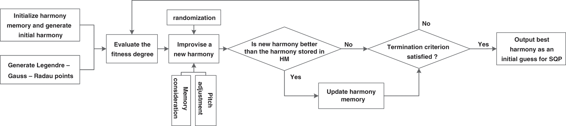
Figure 1: The flowchart of the optimization problem

3.1 Gauss Pseudo-Spectral Method

To solve this discrete Bolza problem requires the use of numerical solution methods. In this paper, a direct spectral collocation method--GPM, is employed to perform the trajectory optimization. In which, the states and the control of an optimal control problem are discretized with some optimal variables at a series of Legendre-Gauss points (LG points) in the time span. And the Lagrange interpolation polynomial is constructed to approximate the state variables and the control variables by using the discrete points as nodes. The terminal state is obtained by the integral of the initial state and the right function in the whole process. By the above transformation, the optimal control problem can be transformed into NLP problem with a series of algebraic constraints.

First of all, the time interval t∈[t0, tf] of the Bolza problem is transformed to τ∈[−1, 1], where the discretized LG points lie in.

τ=2ttf−t0−tf+t0tf−t0 (11)

Then, the continuous Bolza problem through the time transformation is expressed as follows:

J=Φ[x(τ0), τ0, x(τf), τf]+tf−t02∫τ0τfL[x(τ), u(τ), τ]dτs.t.{ dxdτ=t0−tf2f(x(τ), u(τ), τ; t0, tf)ϕ(x(τ0), t0, x(τf), tf)=0C(x(τ), u(τ), τ; t0, tf)≤0(12)

In which, the state and control variables are approximated using a basis of N + 1 Lagrange interpolating polynomials:

x(τ)≈X(τ)=∑i=0KLi(τ)x(τi)u(τ)≈U(τ)=∑i=0KLi(τ)u(τi) (13)

where Li(τ) (i = 1, 2…M) are the Lagrange polynomials of order M, defined as:

Li(τ)=∏j=1,j≠iMτ−τiτi−τj=g(τ)(τ−τi)g˙(τ) (14)

Based on the characteristics of Lagrangian interpolation in Eq. (13), it is very suitable for collocation.

Li(τj)={1i=j0i≠j (15)

To obtain the derivative x˙(τk) in terms of x(τk) at the collocation points τk, the upper equation in Eq. (11) is differentiated and evaluated at τk to make a matrix multiplication of the following form.

x˙(τk)≈X˙(τk)=∑i=0KL˙i(τk)X(τi)=∑i=0KDkiX(τi)(k=1,…,K) (16)

where Dki are the entries of the (N + 1) × (N + 1) differentiation matrix:

Dki=L˙i(τk)={ (1+τk)P˙K(τk)+PK(τk)(τk−τi)[(1+τk)P˙K(τi)+PK(τi)],i≠k(1+τk)P¨K(τi)+2P˙K(τi)2[(1+τk)P˙K(τi)+PK(τi)], i≠k (17)

Based on the above-mentioned state differential approximation, the dynamic differential equation is configured on the LG point (collocation point):

∑i=0KDkiX(τi)−tf−t02f(X(τk),U(τk),τ;t0,tf)=0,(k=1,…,K) (18)

Similarly, the configuration of the kinetic equation on the collocation point, instead of the discrete point, can obtain a higher precision costate variable. And to ensure the consistency, the control variables are also allocated at the LG point. After all, the cost function of the Gauss pseudo-spectral method can be obtained.

J=Φ(X0,t0,Xf,tf)+tf−f02∑k=1Kωig(Xk,Uk,τk;t0,tf) (19)

3.2 The Heuristic Harmony Search

Harmony search is a music-based metaheuristic optimization algorithm. It was inspired by the observation that the aim of music is to search for a perfect state of harmony. It was first proposed by Geem et al. [29], that it imitates the music improvisation process where musicians improvise the pitches of their instruments to obtain better harmony. Compared with the other heuristic optimization algorithm, it is superior in resolving the NLP problem with a better optimal solution in less number of iteration. The harmony search works as follows:

Step 1: Initialize the harmony memory

The harmony memory is important, as it is to choose the best-fit harmony, it can be initialized through a uniform distribution. And a randomly chosen harmony from the HS is initial solution. Besides, relative parameters, namely the harmony memory size, the number of improvisations N, pitch adjusting rate and harmony memory considering rate (HMCR), also need be specified in this step.

Step 2: Improvise a new harmony

Generating a new harmony is called improvisation. The new harmony vector is generated based on the following rules: memory consideration, pitch adjustment and randomization.

In the memory consideration, it is important to assign a HMCR parameter rHMCR ∈ [0,1] to decide how much to choose solution from harmony memory. That is to say, when doing the memory consideration, historical solution from harmony memory will be selected with probability rHMCR. Every solution obtained by the memory consideration is examined with another parameter raccept, which also varies from 0 to 1, to determine whether it should be pitch-adjusted. If raccept is too small, only few best harmonies are selected and it may converge too slowly; if it is too large, almost all the harmonies are used in the harmony memory, then other harmonies are not explored well, leading to potentially wrong solutions. In this paper, raccept is set to 0.85.

The pitch adjustment in music means to change the frequencies; in harmony search, the pitch adjustment is implemented by:

Xnew=Xold+bandrange∗ϵ (20)

where, Xnew is the new pitch with the pitch adjusting action, Xold is the existing pitch or solution from the harmony memory, bandrange a pitch bandwidth, ε is a random number in the range of [−1, 1].

Randomization is to increase the diversity of the solutions. Different from the pitch adjustment, randomization is able to drive the system further to explore various diverse solutions so as to find the global optimality, while the pitch adjustment generally limits to certain local mutation and thus corresponds to a local search.

Step 3: Update the harmony memory

In terms of the obtain value of the fitness function, if the new harmony is better than minimum harmony in harmony memory, include the new harmony in HM, and exclude the minimum harmony from HM.

Step 4: Check the stopping criterion

If stopping criteria (maximum number of improvisations) are not satisfied, go to Step 2; otherwise, terminate the iteration.

4  Numerical Examples

To illustrate the feasibility of presented method in the preceding sections, a number of numerical simulations were carried out. To test the initial guess generator, comparative studies of the harmony search with other intelligent algorithms such as the genetic algorithm (GA) and particle swarm optimization (PSO) are presented. And the three-stage rocket is employed to perform the test, whose vehicle model, optimization model, and constraints establishment are given in Section 2. And the convergence analysis of the proposed method and other algorithms are compared through simulation, and the iteration time is set as 50 for a comprehensive consideration. Fig. 2 shows the iteration results of HS, GA and PSO under the same computational efforts. The results are projected onto the fitness value vs. iteration time plane.

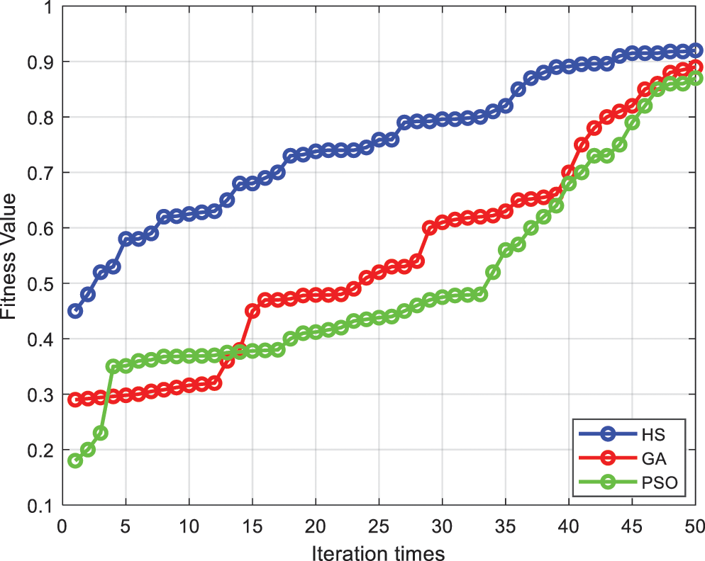
Figure 2: Comparison of convergence capability

As it is seen from Fig. 2, the fitness value of the HS can finally converge to around 0.9, which is very close to 1. And the final value of the fitness function for HS is also higher than its counterparts. Therefore, compared with the GA and PSO, HS is not only lower in complexity, but also performs a better convergence ability and quicker convergence speed. That is to say, by using limited computational efforts, the quality of the initial guess generated by HS algorithm is better than the other two methods that investigated in this paper.

For this study, finding good initial value is to do a good trajectory optimization for the SSO target launch vehicle. After Gauss pseudo-spectral method and the intelligent algorithms, the initial guesses are provided to SQP to solve the optimization problem, the optimized trajectories with different initial generation algorithms are plotted in Figs. 3–6.

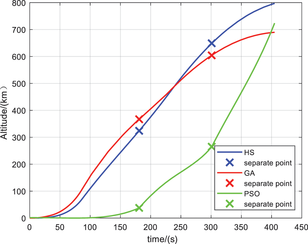
Figure 3: Altitude curve

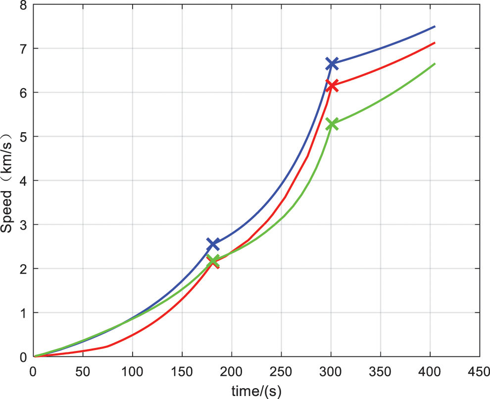
Figure 4: Speed curve

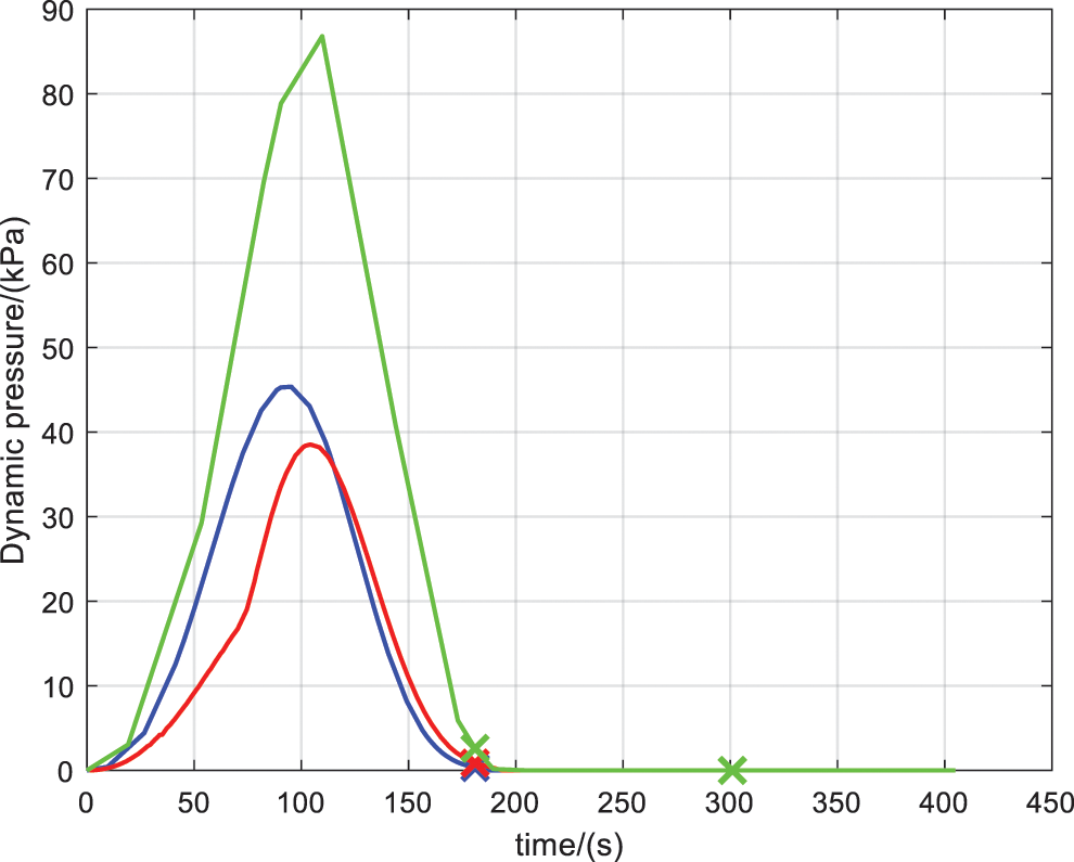
Figure 5: Dynamic pressure curve

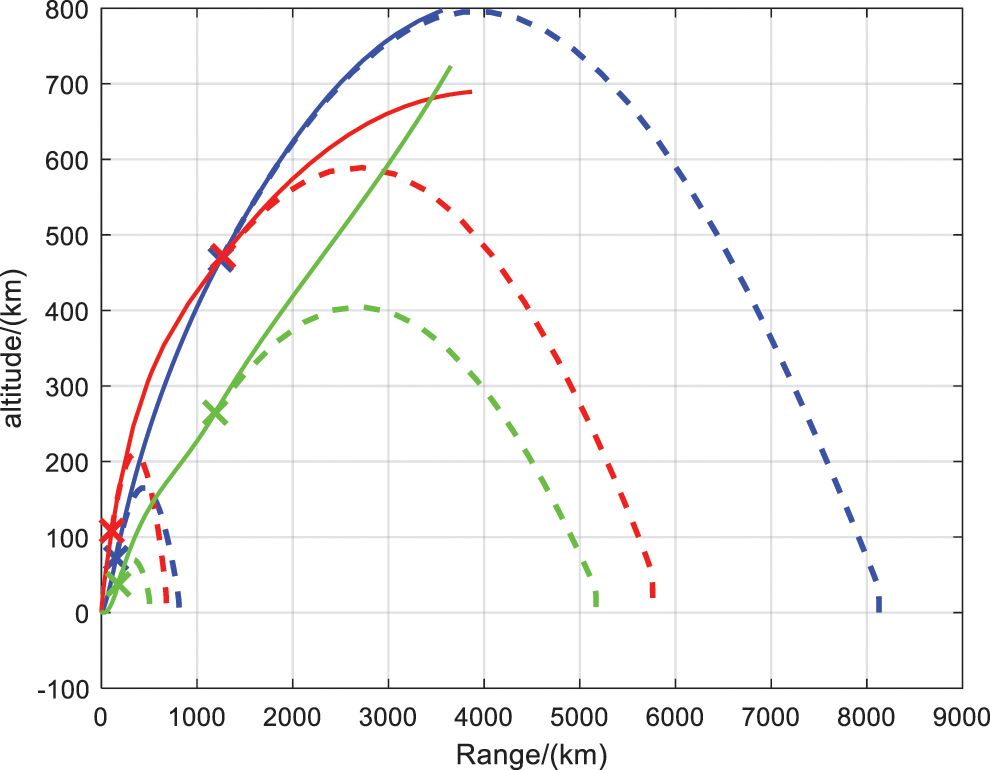
Figure 6: Altitude vs. range

Time histories of altitude and speed are given in Figs. 3 and 4, the terminal altitudes with the three optimized initials are about 800 km, 690 km and 720 km, respectively. And the corresponding terminal speeds are about 7.5 km/s, 7.1 km/s and 6.7 km/s. As the satellite was designed to inject into a sun-synchronous circular orbit, the corresponding altitude and inertial speed should be around 886 km and 7.42 km/s. The comparisons show that the injection with the proposed method is the most nearly optimal in terms of payload mass maximization, since the orbital velocity needed to get into the orbit increases with decreasing altitude. The trajectory quality with HS initial guess generator outperforms the other two manners with higher terminal altitude and speed, which could save more effort for the orbit injection.

Fig. 5 shows the dynamic pressure, while Fig. 6 shows the altitude vs. range including the descent trajectories of the separated stages and the impact points. It is seen that, the dynamic pressure with HS algorithm, GA and PSO are around 45, 38 and 88 kPa, separately. The PSO optimized initial fails to satisfy the constraints of the dynamic pressure. And the corresponding structural mass of the first stage fall at 818 km, 750 and 600 km away from the launch point, only the HS initials agreed with the downrange constraint. Generally, if the initial guess is not close enough to the optimal solution, the performance of gradient-based method is time consuming and it has high probability to converge to local optima.

Based on the intelligent harmony search initial generator, latitude vs. longitude curve of the optimized trajectory is shown in Fig. 7, that the launch vehicle flies from the low latitude to high latitude tries to get into the orbit near the polar region. And the optimized mass profile is given in Fig. 8. It indicates the optimal value of the objective function, clearly, the final mass is obtained as 3345 kg at 405 s. Subtracting the payload mass and the structural mass of the upper stage from the final mass, the remaining fuel is found as 2279 kg that can be utilized as a payload in future missions if the launch vehicle follows the proposed optimal trajectory.

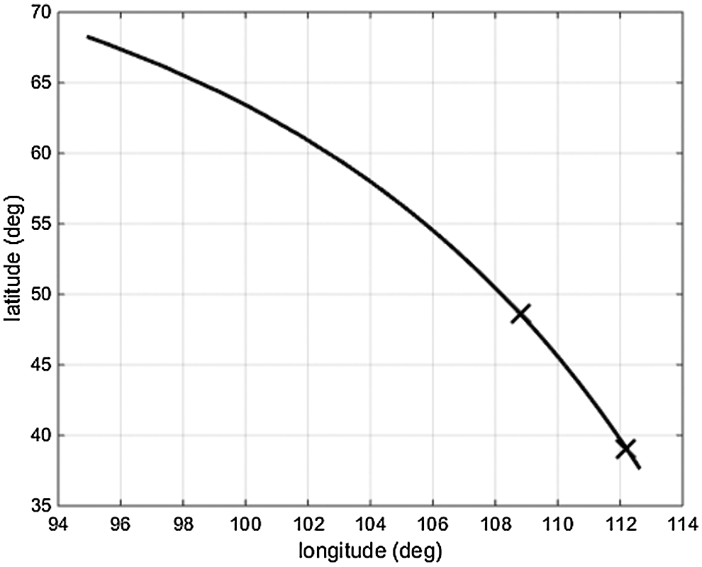
Figure 7: Latitude vs. longitude

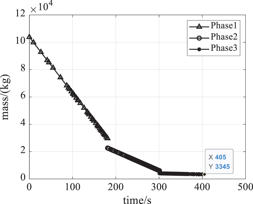
Figure 8: Mass curve

5  Conclusion

In this paper, we solve the trajectory optimization problem for a multistage launch vehicle in consideration of various combinations of dynamic constraints in powering phase. The application of Gauss pseudo-spectral discrete method to three dimensional SSO trajectory optimization problem has been introduced. The optimization problem is modeled and the launch vehicle parameters are present. In order to tackle with the sensitivity of the initial guess for current gradient-based NLP solvers, the intelligent harmony search algorithm is employed. Experimental results show that by applying the initial guess generated using the harmony search, the convergence accuracy for the NLP solver can be improved significantly. Besides, this work could also provide insight into the preferred constraints settings in trajectory optimization for multistage system.

Funding Statement: This work was supported by the National Natural Science Foundation of China (Grant No. 61803203).

Conflicts of Interest: There is no conflict of interests or disclose all the conflicts of interest regarding the manuscript submitted.

This work is licensed under a Creative Commons Attribution 4.0 International License, which permits unrestricted use, distribution, and reproduction in any medium, provided the original work is properly cited.