DOI:10.32604/iasc.2022.023710
| Intelligent Automation & Soft Computing DOI:10.32604/iasc.2022.023710 | |
| Article |
Kidney Tumor Segmentation Using Two-Stage Bottleneck Block Architecture
1Department of Computer Engineering, Kirikkale University, Kirikkale, 71450, Turkey
2Department of Electrical & Electronics Engineering, Kirikkale University, Kirikkale, 71450, Turkey
3Department of Computer Engineering, Faculty of Technology, Gazi University, Ankara, 06560, Turkey
4Department of Electrical & Electronics Engineering, Kirikkale University, Kirikkale, 71450, Turkey
*Corresponding Author: Fuat Turk. Email: turk_fuat@hotmail.com
Received: 18 September 2021; Accepted: 03 November 2021
Abstract: Cases of kidney cancer have shown a rapid increase in recent years. Advanced technology has allowed bettering the existing treatment methods. Research on the subject is still continuing. Medical segmentation is also of increasing importance. In particular, deep learning-based studies are of great importance for accurate segmentation. Tumor detection is a relatively difficult procedure for soft tissue organs such as kidneys and the prostate. Kidney tumors, specifically, are a type of cancer with a higher incidence in older people. As age progresses, the importance of having diagnostic tests increases. In some cases, patients with kidney tumors may not show any serious symptoms until the last stage. Therefore, early diagnosis of the tumor is important. This study aimed to develop support systems that could help physicians in the segmentation of kidney tumors. In the study, improvements were made on the encoder and decoder phases of the V-Net model. With the double-stage bottleneck block structure, the architecture was transformed into a unique one, which achieved an 86.9% kidney tumor Dice similarity coefficient. The results show that the model gives applicable and accurate results for kidney tumor segmentation.
Keywords: Kidney tumors; renal cancer; V-Net model; tumor segmentation
Kidney tumors are among the most common type of urinary tract cancer along with prostate and bladder cancers. It constitutes approximately 2%–3% of adult tumors [1]. Thanks to the technological advances in recent years, an early diagnosis in young patients is possible, especially with the use of ultrasound and computed tomography [2]. According to the report published by cancer statistics in 2018, more than 400,000 kidney cancer cases have been detected worldwide [3]. In addition, most of the diagnosed patients are elderly and the number of asymptomatic kidney tumors is increasing [4]. Weight-related factors such as body mass index (BMI), waist-to-hip ratio (WHR), and waist circumference, as well as external factors such as hypertension and smoking are among the factors directly affecting kidney cancer [5,6].
Benign kidney tumors are generally harmless, but the growth of the mass may represent symptoms such as muscle pain or haematuria (blood in the urine) [7,8]. Malignant kidney tumors are risky and most of them are known as renal cell carcinoma (RCC) [9]. Previously, removal of the entire kidney or tumor tissue seemed to be an effective treatment option. Today, with the increasing importance of imaging techniques, preventive treatment becomes a more preferred option [10]. In recent years, with the increasing use of image recognition and deep learning methods in the field of medicine, medical segmentation has become much more important. However, not much sufficient research kidney tumor segmentation exists in the literature [11–13]. In particular, it is important to conduct more research on the application of artificial intelligence methods in the field of medicine.
U-Net and V-Net models are generally used in segmentation processes in the field of deep learning. Existing multi-scale feature aggregation methods have many problems. One is that it only includes maps with a single encoder and decoder and combines features of the same scale. Another problem is that it performs multiple feature fusions in different encoding and decoding layers. Also, tumor feature information from the same level layer cannot be fully utilized. Fixed-size feature fusion has difficulty learning sufficiently detailed features. Too many nested links and layer structures can also cause some features to be lost. As a consequence, deep network models do not get enough information (as in UNet++). Also, too much heavy hop connection and nesting require using too many parameters. This increases the amount of computation required but does not greatly change the segmentation accuracy. The third problem is that the input is compressed linearly in order to equalize the input and output size, and a bottleneck occurs where all the features cannot be transmitted. Although U-Net and V-Net models try to preserve attributes through incoming connections from the encoder, there are still losses. This study proposes a two-stage bottleneck block structure to overcome such problems.
The aim is to achieve the most accurate results for segmentation by considering the tissue-derived structural features of the kidneys. To this end, a new two-stage V-Net model was developed. Unlike other new approaches, the proposed model was supported by new block structures in the encoder, decoder, and bottleneck stages. The main contributions of the model are:
• Increasing the ability of the encoding phase to capture tumor information through the Squeeze and Excitation (SE) block
• Increasing output accuracy and minimizing feature loss with ResNet++ in decoder phase
• Overcoming the bottleneck problem by the use of a two-stage block structure
• Minimizing loss of feature information through connections between encoder and decoder layers at different levels
• Capturing even the smallest details by being designed with a unique model structure.
The results indicate that the performance of the algorithm is better than its competitors and that the segmentation images are comparable to the data of specialist physicians. Related studies in the literature are explained in Section 2, materials and methods in Section 3, discussion and results are explained in Section 4. Conclusions and future directions form the last part of the study.
Zheng et al. developed a deep learning model called “MDCC-Net”. They stated that multi-scale feature fusion is a suitable method for accurately segmenting the tumor region. According to their study, feature fusion exists only between encoders and decoders of the same scale in some networks. However, in other networks, due to too many layers of nesting and link hopping, some features that might be important may be lost. Therefore, sufficient information may not be learned. To overcome these two problems, they proposed a multi-scale dual-channel evolutionary U-Net model [14].
Cruz et al. emphasized that precise segmentation of kidney tumors would contribute to the diagnosis of diseases and to the improvement of the treatment planning. They also stated that deep learning techniques became popular for the diagnosis of kidney tumors. In their study, they proposed an automated method for delimiting kidneys in computed tomography (CT) images, using image processing techniques and deep convolutional neural networks (CNNs) to minimize the margin of error. The proposed method was tested on 210 CT images from the KiTS19 database and the mean Dice similarity coefficient was found to be 96.33%. Ultimately, they determined the extent of the kidney segmentation problem using deep neural networks and showed that segmenting the kidneys with high precision and using image processing techniques to reduce false positives could solve the problem [15].
Corbat et al., using Artificial Intelligence methods, designed a platform to optimize the segmentation of the deformed kidney and tumor with a small dataset. They combined the segmentation of previously performed structures by using a simple and efficient network. They evaluated the architecture, designed with a fully connected layer structure, on pathological kidney and tumor structures of 14 patients. They emphasized that successful segmentation could be achieved if the results were evaluated on more patients [16].
Qayyum et al. designed a model to perform automatic segmentation of kidney and liver tumors on computed tomography images. They stated that CNN have become important in medical image segmentation tasks in recent years. They proposed a hybrid network model with excitation blocks for segmentation of kidney, liver and associated tumors. In this network structure, SE blocks are preferred to capture spatial information based on the reweighting function. The network model has been tested on the KiTS19 and MICCAI 2017 datasets. The results show that SE blocks can achieve high achievement in volumetric biomedical segmentation [17].
Yin et al. conducted a study for automatic kidney segmentation on ultrasound images. They said that automatic segmentation in ultrasound images is a difficult process due to the shape and image density distributions of the kidney. Researchers proposed a neural network with boundary distance regression and pixel classification operations to automatically segment kidneys. In the classification, kidney border distance maps were taken as input using a border distance regression network. The predicted boundary distance maps split kidney or non-kidney tissue into pixels using a pixel classification network in an end-to-end learning style. The results showed that this method can automatically segment the kidney more successfully than deep learning-based classification networks [18].
Zhao et al. By analyzing CT images, they developed a model called MSS U-Net for 3D segmentation of kidneys and tumors. They stated that accurate segmentation of kidneys and kidney tumors is an important step to develop radiomic analysis and advanced surgical planning techniques. They also reported that nowadays segmentation is performed by visual inspection of images collected by specialist physicians through CT scanning. In the developed architecture, 3D U-Net combines deep control with exponential logarithmic loss value to increase training efficiency. Component-based post-processing method was used to improve the performance of the process. This architecture performed well with kidney and tumor Dice coefficients of up to 0.969 and 0.805, respectively [19].
Turk et al. developed a hybrid V-Net model to segment kidneys and tumors. In the developed model, they aimed to obtain more features from the entrance scene by using the fusion V-Net model in the encoder phase. In addition, they aimed to create clearer output images with ResNet++ architecture in the decoder phase. The developed model was tested on the KiTS19 dataset for kidney and kidney tumor segmentation. The Dice coefficient was found to be 86.5% for tumor segmentation [20].
Turk et al. proposed some improvements on the previously proposed architecture to increase the performance of the U-Net model. In the decoder stage of the U-Net model, the output layer is intensified with nested convolution steps, as in U-Net++. In addition, the output layer is supported by the ResNet++ architecture. The developed model was tested on the KiTS19 dataset for kidney segmentation. The Dice coefficient was 94.9% confirmatory for kidney segmentation and 97.8% for testing [21].
Song et al. proposed a study using the Compressed sensing (CS) algorithm, which provides a general signal acquisition framework that enables the reconstruction of sparse signals from a small number of linear measurements. The current reconstruction block is first predicted by the surrounding reconstructed pixels, and then its prediction residual is reconstructed. Since the sparseness level of the prediction residue is higher than the original image block, the performance of the proposed CS image reconstruction algorithm is significantly superior to the traditional CS reconstruction algorithm. Experimental results show competitive performance of the CS algorithm in terms of highest signal-to-noise ratio and subjective visual quality [22].
Wang et al. have done a study on image classification with the Dense-MobileNet network. In this study, they aimed to achieve less parameters and higher classification accuracy with MobileNet as a lightweight deep neural network. In order to further reduce the number of network parameters and improve classification accuracy, DenseNets recommended dense blocks are included in MobileNet. Thanks to Dense-MobileNet, convolutional layers with same size input feature maps in MobileNet models are taken as dense blocks and dense connections are made in dense blocks. Dense-MobileNet model, Dense1-MobileNet and Dense2-MobileNet were designed. Experiments show that Dense2-MobileNet can provide higher recognition with an accuracy rate of 92.1% [23].
The model proposed in this study is shown in Fig. 1. The model consists of three stages. In the first stage, the encoder phase was transformed into a special design structure with SE blocks so that the architecture could learn the image properties in more detail. In the second stage, the decoder was supported with the ResNet++ architecture to capture even the smallest details in the block output stage. In the last stage, the Non-Local Block + Grid Attention Block (NLB + GAB) structure was integrated into the model in order to overcome the bottleneck problem in convolutional neural networks. The developed architecture is a special design that is not in the literature and contains its own unique features (for codes: https://github.com/turkfuat/Two-Stage-Bottleneck-Block-Architecture).
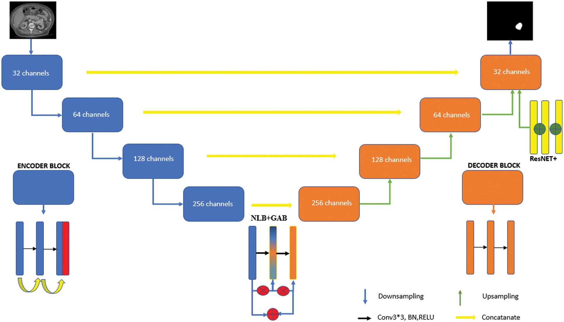
Figure 1: Model architectural structure developed with a two-stage block structure
The classic U-Net architecture consists of two phases. The first one is the encoder stage, which is a stack of convolution and max pool layers aiming to capture the content in the image. The four layers existing in the encoder block are a coding layer, two convolution layer and a RELU layer. Convolution layers are used to get image feature information. Following RELU, max-pooling is used to dilute the feature parameters and reduce the workload (the situation is slightly different for V-Net models). The features in the encoder and decoder stages are combined by Link hops. The biggest challenge here is the processing of the same-scale feature maps in the encoder layer and decoder layer [24,25].
Multiscale feature aggregation steps can facilitate deep learning model to learn detailed features. For example, the U-Net++ architecture can provide multi-scale feature aggregation functionality between the encoder and decode layer via dense hop links. However, too many dense jump connections and nested block layer structure may cause some features to disappear and the characteristic information of the tumor to be learned sufficiently. The workload it brings is another disadvantage. In order to overcome these problems, the developed model was supported with SE blocks in the encoder phase. Encoder phase block structure is seen in Fig. 2. In the first step, the image is entered into the network and after two convolution layers, two-channel separation is applied. A symmetric upsampling process is preferred so that the model can learn the detailed image properties and increase the image size. Thanks to downsampling steps, the image is arranged to be the same size as the input image [26].
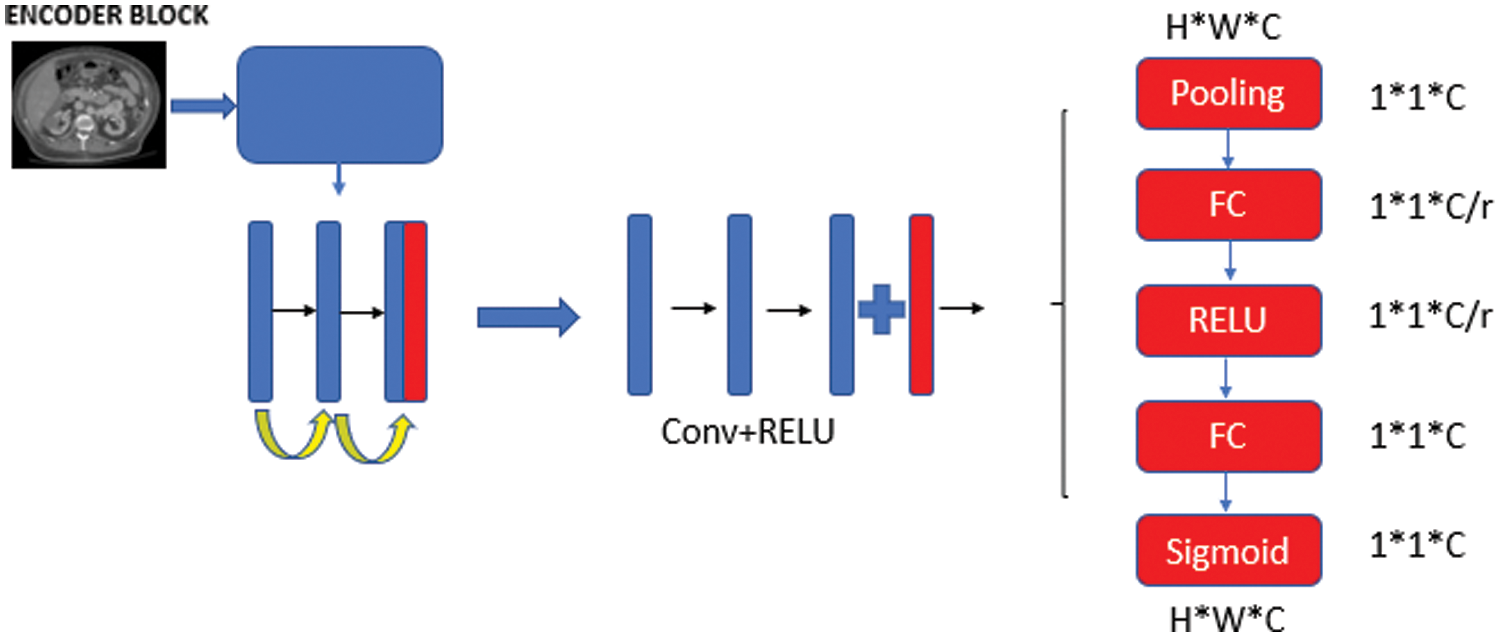
Figure 2: Encoder phase block structure
The SE block was designed to express the relationship between channels [27]. The SE block is used to improve the convolutional features of the architecture by modeling the interdependencies between the channels. The learning level is rearranged to emphasize the informative features of the network and suppress the less qualified ones. A classic SE block structure is shown in Fig. 3.
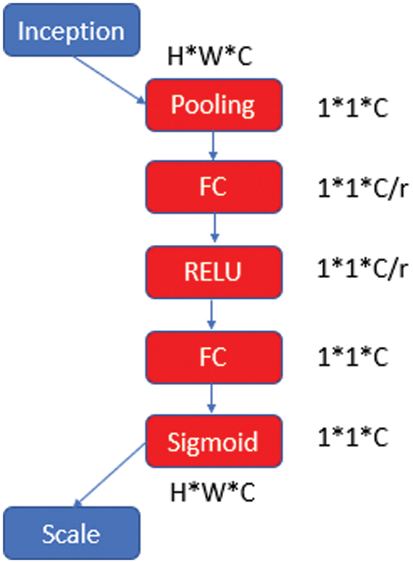
Figure 3: SE block architecture
After the initialization phase, the height (H), width (W), and channel number (C) values are multiplied convolutionally and transferred to the pooling layer and then to the fully connected layer (FC). For dimensional reduction, the C value is divided by a reduction ratio (r). This process is continued with “RELU-FC-Sigmoid” steps and the obtained parameter is rescaled and transferred to the next layer.
SE is a unit of computation with block input
where * denotes the convolution operation, vc the corresponding channel vector, X the input unit. It is aimed to increase the learning of convolutional features by explicitly modeling their interdependencies so that the network can increase its sensitivity to informative features that can be used by subsequent transformations [28,29].
In the decoder stage, the feature map is adjusted to be the same size as the input image using four upsampling block structures. The purpose of maintaining the link between the encoding and decoding layer is to contribute to the discovery of attribute information lost due to convolution layers. Each upsampling block contains an upsampling layer, two convolution layers, a ReLU layer, and a bulk normalization layer. The ResNet++ architecture has been added to the last codec block [20].
This architecture is a system with two nested ResNet blocks integrated. ResNet++ contains differences from the classic ResNet model. The most important difference is that the output layer is linked to the previous two layers. Thus, it is intended to be captured in small details before the output layer. The decoder phase block structure is shown in Fig. 4.
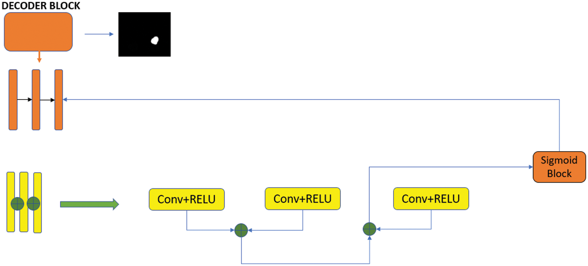
Figure 4: Decoder phase block structure
3.3 Double Stage Bottleneck Block Structure
In deep learning architectures, the size of the input information is regularly reduced in the encoder phase, starting from the first step. The encoder phase is followed by the decoder phase. Linear feature representation is learned in the decoder phase and the size gradually increases. When the decoder phase is finished, the output size is equal to the input size. However, since the input of the system is compressed linearly, a bottleneck occurs where not all attributes can be transmitted. Although the U-Net and V-Net model structures are designed to overcome the bottleneck problems that occur in convolutional neural networks, it is not possible to transmit the input information completely. A two-stage block structure is proposed in order to minimize the loss of input information while transferring it to the output. The designed network architecture is shown in Fig. 5.
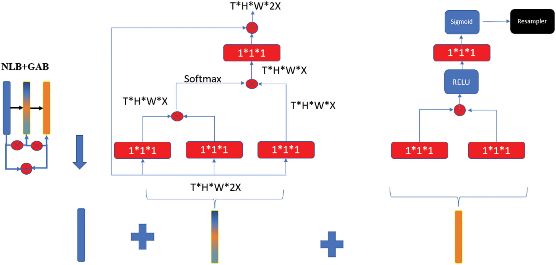
Figure 5: Double-stage bottleneck block structure
In the NLB structure, feature maps are represented as a form of tensors, for example it is expressed as T × H × W × 1024 for 1024 channels. “⊗” stands for matrix multiplication and “⊕” stands for element-wise addition. SoftMax operation is performed on each row. Red boxes show 1 × 1 × 1 convolutions [28]. NLB structure is given in Eq. (2).
where, WZ represents the initial value of the weights, xi represents the residual connection information, yi represents the same size information as xi, and zi represents the block value in the architecture. The bottleneck problem in U-Net architectures can be overcome with single-stage NLB. However, deterioration in image quality at this point will prevent feature losses from being minimized. In order to overcome this problem, the GAB structure was also integrated into the system. In this way, an end-to-end trainable gateway signal is generated and the network is allowed to receive local information useful for prediction from the correct location [29]. In GAB architecture, red boxes show 1*1*1 folds, while “⊕” shows element-wise addition. The folds are resampled with the RELU activation function, first through the single layer structure and then through the sigmoid function.
The Dice Similarity Coefficient (DSC) detects the spatial similarity between two segmentation units or how much they overlap [30]. It is a common metric used to compare segmentation performance with baseline truth in medical images [31]. The Jaccard Index, also known as the Jaccard similarity coefficient, is a statistical value used to determine the proportion of similarities between sample sets. The measurement highlights the similarity between finite sets of samples and is defined as the intersection size divided by the size of the union of sample sets [32]. These two evaluation criteria are shown in Fig. 6. DSC equation is indicated in Eq. (3) and Jaccard index is indicated in Eq. (4).

Figure 6: Display of DSC and Jaccard index domain calculation
A, represents the result of the segmentation, whereas B represents the corresponding absolute reference image. In general, a comparison is made between the segmentation accuracy and the results of segmentation methods [33].
In this study, 210 datasets available for public access and downloadable from the cancer imaging archive (https://www.cancerimagingarchive.net/) were used [34]. The clinical features, imaging data, kidney and tumor boundaries of the existing patients were prepared by using the manual segmentation method. In Fig. 7, an example segmentation prepared with this method is shown.
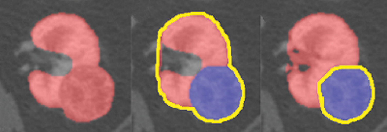
Figure 7: A kidney image prepared by manual segmentation
In the first step, the CT images in the dataset were resized to 16 × 256 × 256 and divided by 255 to normalize the pixel values between 0 and 1. For training, patches sized 64 × 128 × 128 were randomly selected from the resampled data. Out of a total of 210 datasets, 190 were used for training and 20 for testing. The Adam Optimizer algorithm was preferred for model training and the learning coefficient was taken as 0.001. The batch size was set to 3 and the total steps were set to 100,000. The training of the model took approximately 96 h on the NVIDIA Tesla V100 Graphics Processing Unit (GPU). TensorFlow library features were used during the training.
U-Net, U-Net++, V-Net and the developed two-stage block model were run with the same hyperparameters and the results are discussed in detail below. The data shown here are the average of the five-fold cross-validation results run on the dataset. Fig. 8 shows the algorithm for our five-fold cross-validation structure.

Figure 8: 5-fold cross validation algorithm for the model
Fig. 9 shows the DSC and loss graphs of the developed model. The validation loss continues to decrease as the training loss decreases, indicating that the proposed method learns without memorization. The sudden changes in the initial steps of the training decrease to an acceptable level in the following steps, indicating consistent training.

Figure 9: DSC and loss graph during the training period
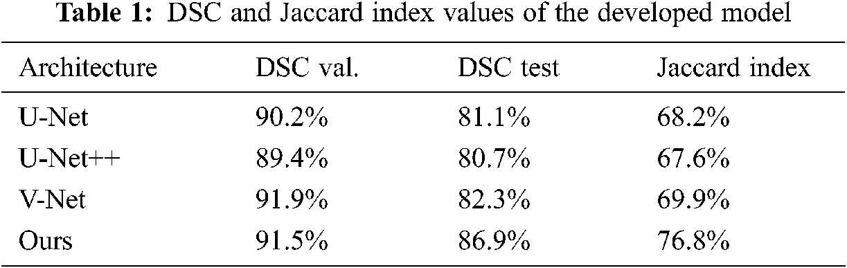
Dice coefficients and Jaccard index values obtained from validation and test results are shown in Tab. 1 The results show that the developed model outperforms other advanced networks on most evaluation indicators. The validation and test results are also close and consistent.
Tab. 2 shows a comparison of the results of this study with the results from the KiTS19 Challenge and the results from the literature. In the literature research, the current studies that are closest in terms of content and subject to this study were discussed. 90 datasets in the KiTS19 Challenge were not evaluated because they were publicly inaccessible. As with other studies, those excluded from the dataset due to mislabeling were also used. No changes were made to the dataset in order to compare the results obtained with other future studies. Other studies compared to this study are given below.
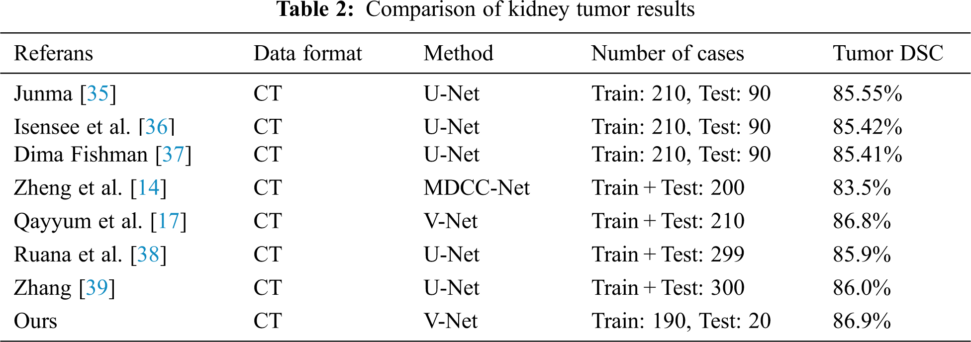
Junma developed a U-Net-model using the dataset from Kits19 Challenge and achieved the best result with the kidney tumor Dice coefficient value in the Challenge. He obtained a Dice coefficient value of 85.55% for kidney tumour segmentation [35].
Isensee et al. [36] developed a U-Net model and achieved a Dice Coefficient of 85.42% for kidney tumour segmentation.
Dmytrofishman developed a U-Net model and achieved a Dice Coefficient of 85.41% for kidney tumour segmentation [37].
Zheng et al. developed a U-Net-based model, which they named MDCC-Net. They tested the model on the dataset consisting of 200 CT images in the KiTS19 Challenge, and they succeeded in reaching a Dice Coefficient of 83.5% for kidney tumour segmentation [14].
Qayyum et al. [17] developed a V-Net-based model achieving 86.8% Dice Coefficient for kidney tumour segmentation on the KiTS19 dataset.
Ruana et al. used a U-Net-based model, which they named MB-FSGAN. They tested the model on a dataset of 113 CT images and achieved a Dice Coefficient of 85.9% for kidney tumour segmentation [38].
Zhang et al. used U-Net based model, which based model nnU-Net. They tested model on a KiTS21 Challenge dataset of 299 CT images and achieved a Dice Coefficient of 86.0% for kidney tumour segmentation [39].
Fig. 10 shows the original images and masks used for kidney tumor segmentation as well as the segmentation results of the model developed in this study and the other models compared. The results of the comparison made with the U-Net and V-Net models, which show high education and test success, are very close to each other. However, when we look carefully, we can see that our model yields better results than existing V-Net models in detecting small details and tumor outer borders. The model we developed with the changes made to capture the image features and details and to solve the bottleneck problems yielded positive and successful results.
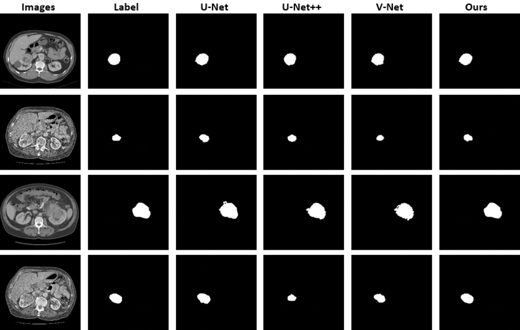
Figure 10: CT images and images obtained as a result of kidney tumor segmentation
Segmentation with deep learning is of high importance for the early diagnosis of tumors difficult to detect in soft tissues such as kidney tumors. This study presents a comparison of U-Net and V-Net models used to segment kidney tumor regions. All architectures were trained on the dataset in the KiTS19 Challenge. The developed model achieved a DSC score of 91.5% for validation and 86.9% for testing, yielding the best results of the compared networks.
In this study, more tumor information could be captured at the coding stage thanks to SE blocks. With the two-stage block structure, the bottleneck problem was partially overcome. With the layer structure at different levels, feature information can be minimized. Furthermore, changes were made to 3 fundamental parts of the U-Net architecture. The encoder phase, decoder phase, and bottleneck stages were designed separately. All of the designed architectures were used together and for the first time, and had a high success rate. The applicability of different modifications of the U-Net and V-Net models to the KiTS19 Challenge dataset was also demonstrated. The model we developed, if taken as a reference, can lead to the design of faster and more accurate architectures than existing networks in the coming years. The design and development of deep learning architectures is a difficult engineering task that requires the selection of many new hyperparameters and layer configurations. However, the structure of the SE block is quite simple, computationally light, and the workload is quite low. With state-of-the-art architectures, SE block performance can be effectively increased and be made directly usable.
This study can be a guide for future models, as it shows that the ResNet++ architecture can yield more successful results when properly integrated into non-complex models in image segmentation studies. To sum up, this paper proposes a new architecture to accurately determine tumor boundaries through the two-stage block structure used to minimize the loss of bottleneck-induced features. The results also suggest that increasing the complexity, the number of layers, or the depth of a network (like U-Net++) may not always yield better results. Further research studies on hyperparameters may be a more rational approach to increase network success.
The network architecture structure developed in this study will be tested for segmentation in other tumor tissues, especially in multiple kidney tumors, if the appropriate dataset is found. The results to be obtained will hopefully make an important contribution to the literature and the field of medicine for the detection of tumors in tumor tissues at an early stage.
Funding Statement: This research was conducted without financial support.
Conflicts of Interest: The authors declare that they have no conflicts of interest to report regarding the present study.
1. H. Sung, J. Ferlay, R. L. Siegel, M. Laversanne, I. Soerjomataram et al., “Global cancer statistics 2020: GLOBOCAN estimates of incidence and mortality worldwide for 36 cancers in 185 countries,” A Cancer Journal for Clinicians, vol. 71, no. 3, pp. 209–249, 2021. [Google Scholar]
2. D. Teber, T. Erdoğru, J. Klein, T. Frede and J. Rassweiler, “Laparoscopic radical nephrectomy: Surgical outcomes and longterm oncologic follow-up,” Turk Uroloji Dergisi, vol. 31, no. 1, pp. 41–48, 2005. [Google Scholar]
3. Z. Du, W. Chen, Q. Xia, O. Shi and Q. Chen, “Trends and projections of kidney cancer incidence at the global and national levels, 1990–2030: A Bayesian age-period-cohort modeling study,” Biomarker Research, vol. 16, pp. 8, 2020. [Google Scholar]
4. N. Heller, N. Sathianathen, A. Kalapara, E. Walczak, K. Moore et al., “300 kidney tumor cases with clinical context, CT semantic segmentations, and surgical outcomes,” arXiv preprint arXiv: 1904.00445v2, 2019. [Google Scholar]
5. S. Wang, M. D. Galbo, C. Blair, B. Thyagarajan, K. Anderson et al., “Diabetes and kidney cancer risk among post-menopausal women: The Iowa women’s health study,” Maturitas, vol. 143, pp. 190–196, 2020. [Google Scholar]
6. T. Pischon, P. H. Lahmann, H. Boeing, A. Tjonneland, J. Halkjaer et al., “Body size and risk of renal cell carcinoma,” The European Prospective Investigation into Cancer and Nutrition (EPIC) International Journal of Cancer, vol. 118, no. 3, pp. 728–738, 2006. [Google Scholar]
7. S. Tangal, K. Önal, M. Yığman and A. H. Haliloğlu, “Relation of neutrophil lymphocyte ratio with tumor characteristics in localized kidney tumors,” The New Journal of Urology, vol. 13, no. 1, pp. 12–15, 2018. [Google Scholar]
8. M. Sun, F. Abdollah, M. Bianchi, Q. D. Trinh, C. Jeldres et al., “Treatment management of small renal masses in the 21st century: A paradigm shift,” Annals of Surgial. Oncology, vol. 19, pp. 2380–2387, 2012. [Google Scholar]
9. G. Yang, J. Gu, Y. Chen, W. Liu, L. Tang et al., “Automatic kidney segmentation in ct images based on multi-atlas image registration,” in Proc. of the 36th Annual Int. Conf. of the IEEE Engineering in Medicine and Biology Society, Chicago, IL, USA, pp. 5538–5541, 2014. [Google Scholar]
10. D. Mohanapriya and B. Kalaavathi, “Adaptive image enhancement using hybrid particle swarm optimization and watershed segmentation,” Intelligent Automation and Soft Computing, vol. 25, pp. 663–672, 2019. [Google Scholar]
11. S. Calıskan, O. M. Koca and M. I. Akyuz, “Böbrek tümörü öntanısıyla radikal veya parsiyel nefrektomi yapılan hastalardaki benign tümörler,” The New Journal of Urology, vol. 9, no. 1, pp. 34–37, 2014. [Google Scholar]
12. M. C. Mir, I. Darwish, F. Porpiglia, H. Zargar, A. Mottrie et al., “Partial nephrectomy versus radical nephrectomy for clinical t1b and t2 renal tumors: A systematic review and meta-analysis of comparative studies,” Europen Urology, vol. 71, no. 4, pp. 606–617, 2017. [Google Scholar]
13. Q. Yu, Y. Shi, J. Sun, Y. Gao, Y. Dai et al., “A novel convolutional network for kidney tumor segmentation in CT images,” arXiv preprint arXiv: 1804.10484, 2020. [Google Scholar]
14. S. Zheng, X. Lin, W. Zhang, B. He, S. Jia et al., “MDCC-Net: Multiscale double-channel convolution U-Net framework for colorectal tumor segmentation,” Computers in Biology and Medicine, vol. 130, pp. 104183, 2021. [Google Scholar]
15. L. B. Cruz, J. D. Lima, J. L. Ferreira, J. O. Diniz, A. C. Silva et al., “Kidney segmentation from computed tomography images using deep neural network,” Computers in Biology and Medicine, vol. 123, pp. 103906, 2020. [Google Scholar]
16. L. Corbat, J. Henriet, Y. Chaussy and J. Lapayre, “Fusion of multiple segmentations of medical images using OV2 ASSION and deep learning methods: Application to CT-scans for tumoral kidney,” Computers in Biology and Medicine, vol. 124, pp. 103928, 2020. [Google Scholar]
17. A. Qayyum, A. Lalande and F. Meriaudeau, “Automatic segmentation of tumors and affected organs in the abdomen using a 3D hybrid model for computed tomography imaging,” Computers in Biology and Medicine, vol. 127, pp. 104097, 2020. [Google Scholar]
18. S. Yin, Q. Penga, H. Li, Z. Zhanga, X. Youa et al., “Automatic kidney segmentation in ultrasound images using subsequent boundary distance regression and pixelwise classification networks,” Medical Image Analysis, vol. 60, pp. 101602, 2020. [Google Scholar]
19. W. Zhao, D. Jiang, J. Pena and T. Westerlund, “MSS U-Net: 3D segmentation of kidneys and tumors from CT images with a multi-scale supervised U-Net,” Informatics in Medicine Unlocked, vol. 19, pp. 100357, 2020. [Google Scholar]
20. F. Turk, M. Luy and N. Barıscı, “Kidney and renal tumor segmentation using a Hybrid V-Net-Based model,” MDPI Mathematics, vol. 8, no. 10, pp. 1772, 2020. [Google Scholar]
21. F. Turk, M. Luy and N. Barisci, “Renal segmentation using an improved U-Net3D model,” Journal of Medical Imaging and Health Informatics, vol. 11, no. 8, pp. 2258–2266, 2021. [Google Scholar]
22. Y. Song, W. Cao, Y. Shen and G. Yang, “Compressed sensing image reconstruction using intra prediction,” Neurocomputing, vol. 151, no. 3, pp. 1171–1179, 2015. [Google Scholar]
23. W. Wang, Y. T. Li, T. Zou, X. Wang, J. Y. You et al., “A novel image classification approach via Dense-MobileNet models,” Mobile Information Systems, vol. 2020, pp. 7602384, 2020. [Google Scholar]
24. D. G. Stanislav, P. S. Victor and A. B. Artem, “Comparative analysis of the usage of neural networks for sound processing,” in IEEE Conf. of Russian Young Researchers in Electrical and Electronic Engineering (EIConRus), St. Petersburg and Moscow, Russia, 2020. [Google Scholar]
25. F. Turk, M. Luy and N. Barıscı, “Comparison of U-Net and U-Net+ResNet models for kidney tumor segmentation,” in 3rd Int. Symp. on Multidisciplinary Studies and Innovative Technologies, Ankara, Turkey, 2019. [Google Scholar]
26. J. Hu, L. Shen, S. Albanie, G. Sun and E. Wu, “Squeeze-and-excitation networks,” IEEE Transactions on Pattern Analysis and Machine Intelligence, vol. 42, no. 8, pp. 2011–2023, 2020. [Google Scholar]
27. A. G. Roy, N. Nava and C. Wachinger “Concurrent spatial and channel ‘Squeeze & Excitation’ in fully convolutional networks,” in Medical Image Computing and Computer Assisted Intervention (MICCAI), Springer, Granada, Spain, vol. 11070, pp. 412–429, 2018. [Google Scholar]
28. X. Wang, R. Girshick, A. Gupta and K. He, “Non-local neural networks,” in Proc. of the IEEE Conf. on Computer Vision and Pattern Recognition (CVPR), Salt Lake City, Utah, pp. 7794–7803, 2018. [Google Scholar]
29. J. Schlemper, O. Oktay, L. Chen, J. Matthew, C. Knight et al., “Attention gated networks: Learning to leverage salient regions in medical images,” Medical Image Analysis, vol. 53, pp. 197–207, 2019. [Google Scholar]
30. C. H. Sudre, W. Li, T. Vercauteren, S. Ourselin and M. J. Cardoso, “Generalized dice overlap as a deep learning loss function for highly unbalanced segmentations,” Deep Learning in Medical Image Analysis and Multimodal Learning for Clinical Decision Support (DLMIA), vol. 10553, pp. 240–248, 2017. [Google Scholar]
31. S. Chen, R. Holger, O. Hirohisa, O. Masahiro, H. Yuichiro et al., “On the influence of dice loss function in multi-class organ segmentation of abdominal CT using 3D fully convolutional networks,” arXiv preprint arXiv: 1801.05912, 2018. [Google Scholar]
32. M. Bouchard, A. L. Jousselme and P. E. Doré, “A proof for the positive definiteness of the Jaccard index matrix,” International Journal of Approximate Reasoning, vol. 54, pp. 615–626, 2013. [Google Scholar]
33. S. Andrews and G. Hamarneh, “Multi-region probabilistic dice similarity coefficient using the Aitchison distance and bipartite graph matching,” arXiv preprint arXiv: 1509.07244, 2015. [Google Scholar]
34. The Cancer Imaging Archive (TCIA2021. [Online]. Available: https://wiki.cancerimagingarchive.net/pages/viewpage.action?pageId=61081171. [Google Scholar]
35. KiTS19 Challenge Org., Junma, 2021. [Online]. Available: https://grand-challenge.org/users/junma/. [Google Scholar]
36. N. Heller, F. Isensee, K. H. Marier-Hain, X. Hou, C. Xie et al., “The state of the art in kidney and kidney tumor segmentation in contrast-enhanced CT imaging,” Medical Image Analysis, vol. 67, pp. 101821, 2021. [Google Scholar]
37. KiTS19 Challenge Org., Dima Fishman, 2021. [Online]. Available: https://grand-challenge.org/users/dmytrofishman/. [Google Scholar]
38. Y. Ruana, D. Li, H. Marshall, T. Miao, T. Cossetto et al., “MB-FSGAN: Joint segmentation and quantification of kidney tumor on CT by the multi-branch feature sharing generative adversarial network,” Medical Image Analysis, vol. 64, pp. 101721, 2020. [Google Scholar]
39. KiTS21 Challenge Org., Zhang, 2021. [Online]. Available: https://kits21.kits-challenge.org/results. [Google Scholar]
 | This work is licensed under a Creative Commons Attribution 4.0 International License, which permits unrestricted use, distribution, and reproduction in any medium, provided the original work is properly cited. |