DOI:10.32604/iasc.2022.022972
| Intelligent Automation & Soft Computing DOI:10.32604/iasc.2022.022972 | |
| Article |
An Advanced Integrated Approach in Mobile Forensic Investigation
1Department of Computer Science and Engineering, Saveetha Engineering College, Chennai, 602105, India
2Department of Computer Science and Engineering, School of Computing, SRM Institute of Science and Technology, Chengalpattu, 603203, India
3Department of Information Technology, Saveetha Engineering College, Chennai, 602105, India
*Corresponding Author: G. Maria Jones. Email: joneofarc26@gmail.com
Received: 24 August 2021; Accepted: 09 October 2021
Abstract: Rapid advancement of digital technology has encouraged its use in all aspects of life, including the workplace, education, and leisure. As technology advances, so does the number of users, which leads to an increase in criminal activity and demand for a cyber-crime investigation. Mobile phones have been the epicenter of illegal activity in recent years. Sensitive information is transferred due to numerous technical applications available at one’s fingertips, which play an essential part in cyber-crime attacks in the mobile environment. Mobile forensic is a technique of recovering or retrieving digital evidence from mobile devices so that it may be submitted in court for legal procedures. As a result, mobile phone data is essential for obtaining evidence in elements of mobile forensic data analysis. So, in this paper, we offer a method for detecting suspect drug-dealing patterns in mobile devices utilizing forensic and Natural Language Processing (NLP) techniques. Machine Learning algorithms are used to uncover the pattern in an original dataset, and performance measurements are used to assess the suggested system. In our approach, Logistic Regression (LR) manifests 95% of the highest accuracy in terms of count vector whereas, the BiLSTM (Bidirectional Long Short Term Memory) also achieved 95% of accuracy in terms of TFIDF.
Keywords: Mobile forensic; digital evidence; suspicious patterns; machine learning; time series
In digital forensic, extracting digital evidence from a mobile device is a novel and evolving technology. Digital forensic is a critical tool for identifying and gathering evidence related to a variety of criminal acts. Reconstructing, recovering, and examining past events or raw data stored in electronic devices are the subjects of digital forensic. The goal of digital forensic is to retrieve data from any electronic device without changing, deleting, adding, or manipulating the data. Digital forensic, like computers and other digital devices, has advanced fast during the last decade [1]. Computer Forensic, Database Forensic, Mobile Forensic, Cloud Forensic, Memory Forensic, Network Forensic, and so on are the types of digital forensic. According to Ericsson’s research, data traffic will reach 71 exabytes per month in 2022, from 8.8 exabytes in 2017 Cyber crimes are defined as crimes committed using computer systems [2]. At the crime scene, every criminal behaviour tends to leave digital imprints. Digital evidence is usually found in digital devices and can also be obtained through social media. Mobile devices, computers, laptops, and tablets are used to commit the crime, and digital evidence is kept or communicated to other devices that may aid in proving the guilt.
Evidence can be found on a computer hard drive, a mobile device, an SD card, and other devices. These are linked to online crimes such as credit card fraud, pornography, and different types of cybercrime. Apart from that, email plays a crucial role in many cases, as it may include key evidence relevant to the case. These digital footprints are detectable on the internet and are primarily used to identify criminal activity. They can range from internet caches, log files, emails, conversations, and documents, among other things. Since mobile technologies are becoming more sophisticated, leaving footprints is an unavoidable possibility. During a mobile forensic examination, many storage configurations on smartphones are investigated. During a crime scene investigation, however, the amount of digital data generated increases inexorably. Mobile forensic technologies are used to collect data and evaluate digital evidence in majority of illegal actions. Mobile forensic is a sub-branch of digital forensic that uses a forensically sound flow process to recover/reconstruct the past events of digital evidence from mobile devices. To protect its integrity and secrecy, digital proof should be acquired in a forensically sound manner, which means copying the original data bit by bit without changing the primary substance [3]. The evidence gathered may be incomprehensible, but it can be made understandable with the help of mobile forensic technologies. Correlating data from various file types is a time-consuming activity.
This research aims at using forensic processes and Machine Learning Techniques (MLT) to analyse criminal actions, including drug distribution, particularly in mobile devices. The NLP techniques can be used to identify keywords from text messages of dealers and clients. Machine learning algorithms are used to analyze SMS (Short Message Service) and call records in a drug-selling dataset using mobile devices and to evaluate performance measures for recognizing suspect call and message log patterns. Because of technical advancements, the growth of digital data has been enormous. According to the author [4], digital devices with the internet have a part in the rise in the number of criminal cases, and in this scenario, machine learning (ML) and deep learning (DL) algorithms help with smart forensic investigation. According to the National Survey on Drug Use and Health (NSDUH), over 9.4 percent of Americans aged 12 and alone took drugs in 2003, compared to 8.3 percent in 2003 [5]. As a result, there is a definite increase in illicit drug consumption in the United States. This article presents a novel method for analysing the behavioural pattern of drug peddlers and drug customers communicating over mobile phones.
The following works are the main contribution of this paper.
1. We study the current state of mobile device forensic with the traditional flow process of digital forensic.
2. We present a literature review of mobile forensic and MLT from the research community incorporated into the design of standard flow process and perform mobile forensic investigation.
3. Examining and extracting related keywords to identify the messages of dealers and clients.
4. Encompassing Forensic techniques and ML algorithms to review demographics and detect user behavioural patterns.
5. The time series algorithms are used for prediction based on the message exchanged between dealer and client by means of LSTM (Long Short Term Memory), ARIMA (Autoregressive Integrated Moving Average), and SARIMA (Seasonal Autoregressive Integrated Moving Average) algorithms.
6. We present an evaluation metrics of the proposed work for mobile forensic data that could help examiners to identify the behavioural pattern.
The rest of the article is organized as follows; Section 2 presents relevant works on mobile forensic, machine learning, NLP, and drug dealing. Section 3 describes the proposed methodology of the integrated approach of the forensic system. Section 4 presents the text-based classifier in identifying dealers and client accounts from a mobile device and is analyzed using ML and Evaluation Metrices. Section 5 presents the implementation of time series algorithms. Section 6 evaluates the results and provides a discussion of the work. Finally, the conclusion is presented in Section 7.
A substantial amount of research is recorded to analyze and acquire digital evidence from mobile environments, especially in the drug dealing process with machine learning techniques. The authors used text processing methodology to represent the relevant key concepts based on semantic web principles in computer forensic. They intended to improve the performance with the help of machine learning and multimedia techniques aiming for representing the multimedia resources as future work [6]. The authors proposed a machine learning technique called diverging deep learning cognitive computing technique into the cyber forensic framework to assist the forensic investigators and concluded with a future prospect of developing DL algorithms to manage the investigation process [7]. About 20 Android applications were investigated through network and storage analysis wherein passwords, pictures, videos, messages etc., were retrieved but failed to reconstruct the chat from Snapchat, tinder, wicker, or BlackBerry Messenger (BBM) [8]. The work offers a framework called DERDS (Digital Evidence Reporting and Decision Support) to identify the potential digital evidence and discuss structure and application with decision-making demonstration [9].
The article explains digital evidence acquisition from social media forensic along with the challenges involved during the process of collection, analysis, presentation, and validation in legal processing with recent research gaps, objectives and provided a research direction [10]. The authors retrieved the data from Microsoft skype application inorder to identity the end user by analyzing the CODEC which is transferred by the client at the time session initiation protocol [11]. The work explained that how seven different types of machine learning models helps to trace the file system and also helped to analyse how the files can be altered. The authors also used performance measures to identify the best model, whereas random forest showed highest accuracy among others [12]. The researchers [13] presented structural feature extraction methods to detect malicious features which resides in a documents by using machine learning models, The author presented a majorclust algorithm to detect suspicious activities in logs, which assists forensic examiner in inspecting the log files and achieved 70.59%, 82.21%, and 83.14% of sensitivity, specificity, and accuracy, respectively [14].
3 The Integration Model of ML and DL Algorithms with Mobile Forensic
In this section, a novel framework for Mobile Device Forensic is proposed using machine learning techniques to analyse the text messages which could be helpful for law enforcement. In the initial stage of the proposed work, the mobile forensic toolkit is used to collect the user information from a mobile device. The data retrieved from a mobile device using an oxygen forensic toolkit can be stored in structured file format, namely CSV, HTML, XML, etc. This paper describes the architecture and implementation of machine learning techniques to analyze the crime pattern in drug dealing and the forensic techniques used to detect crime-related suspicious activities. The working process of the proposed system is shown in Fig. 1, wherein data collection is a significant task in the analysis.
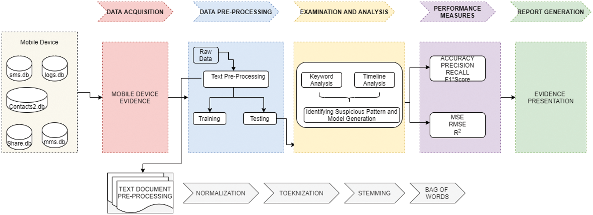
Figure 1: Architecture diagram for the proposed system
Even though most forensic tools work with the plain text, they do not have advanced analysis techniques. In Fig. 1, the initial module called “Mobile Device Evidence” acquires the data bit by bit copy of the mobile device. The module extracts relevant information from the database like messages, contact, user files, etc. In our model, we aim to extract the text data correlated with illicit drug keywords. So, the second module is designed for pre-processing the text as it is used for further analysis. The third module is used to identify the suspicious pattern and model generation using ML and DL methods. The ML and DL methodologies can be expensively used for determining the behavioural pattern. For each model generation, the performance measures are calculated, and the final stage is report generation which presents the final documents to juries. The purpose of the presentation is to provide the report comprising tools, scientific techniques, and methodologies used to collect the evidence and to briefly illustrate the actions taken.
In Forensic Terminology, data collection can also be called evidence collection for digital investigation. There are three types of methods employed for data acquisition in mobile forensic. They are Logical Acquisition, Physical Acquisition and manual acquisition. In this paper, the logical acquisition method is used to analyze illicit drug-related keywords from text content. The work deals with analyzing and exploring the evidence from a mobile device. Data collection is the crucial part for every examiner. Mobile evidence is retrieved using the Oxygen Forensic toolkit. Based on the keywords like “weed”, “Oxy”, “Pills”, etc., the authors retrieved all relevant text contents and analyzed them by sentimental analysis. The time series analysis of the chats between drug dealers and clients over the years are also employed. The dataset was obtained through mobile device with instances of 10625 text messages where tuples are Message-Id, Time, Date, Text, and class. For time series analysis, the dataset comprised around 300 instances.
The process involved in Pre-processing is termed as the process of cleaning raw data before implementing Machine Learning algorithms. Text Pre-processing ensures the elimination of noisy data from the data set. Before encoding the text into a numeric vector, the pre-processing is implemented with the assistance of the following techniques: Eliminating URL, converting all uppercase characters to lower case, Eliminating unwanted characters like punctuation, removing stop words, stemming and lemmatization, Normalization, and many more techniques.
To understand the behaviour of drug peddlers in mobile device chat-logs, we conducted several experiments with the real-time dataset to extract features that explain how machine learning and deep learning models would identify the peddlers conversations. This enabled us to provide insightful information that can be useful for forensic investigations. To that end, we trained the specific ML, and DL supervised algorithms. We utilized four ML models and one DL model: Multinomial Naïve Bayes, Logistic Regression, Support Vector Machine, and XGBoost in ML and Long Short Time Memory in DL algorithms.
Multinomial Naïve Bayes model is a probabilistic ML algorithm which is used to classify a wide variety of classification task mostly used in Natural Language Processing.
XGBoost is termed as eXtreme gradient boosting used to implement the gradient boosting trees which are designed to improve the speed and performance of the system. It works on the problems like classification, Regression, user-defined prediction (unstructured data) and ranking.
SVM is supervised learning which can perform both classification and regression problems. The hyperplanes are used to classify the whole dataset into groups based on similar patterns [15]. The main objective is to find out the plane with a maximum margin which helps for future classification.
Logistic Regression is used for classification problems that work on a cost function called the sigmoid function which is used to map numbers to probabilities. Logistic Regression is also used for regression methods for solving both binary and multinomial classification problems. A detailed explanation of LSTM is described in Section 5.2.
3.4 Validation and Performance Measures
Performance evaluations for Machine Learning algorithms are essential to quantify the performance of each algorithm. The performance evaluation is based on a machine learning task like classification algorithms, Regression, Topic Modeling, etc. The performance metrics are evaluated by Precision, Recall, F1 Score, Accuracy, AUC (Area Under Curve), ROC (Receiver Operating Characteristic) for Classification problem and MAE (Mean Absolute Error), MSE (Mean Square Error) and R2 (R-Squared) is used to calculate the performance for Regression related problems.
The report presentation phase is the investigation’s final stage, wherein all the relevant evidence is presented in court. The report is presented manually in court because the jury and the lawyers will decide about appropriate digital evidence based on legal proceedings. One of the investigators’ main challenges is to explain the digital data, evidence gathered, and the results obtained to non-technical persons. So, the report can be aided with possible visualizations, charts, and graphs for better understanding. The examiners choose the valid evidence or information that meets the motivation of the investigation.
4 Text-Based Classifier Using Mobile Forensic
Mobile forensic is a branch of digital forensic which is utilized to retrieve digital evidence from mobile phones. Smartphones have become an integral part of one’s daily routine, so they are prone to facilitate and be involved in criminal activities. Several mobile forensic toolkits can retrieve suspicious evidence from mobile phones, namely Encase, Oxygen forensic, Belkasoft, Cellebrite’s Universal Forensic Extraction Device (UFED), SANS OSForensics, XRY Forensic Examiner’s Kit, Access data, etc. In this section, the authors used forensic software to retrieve drug-related keywords in the text, analyzed the messages by WordCloud, and used machine learning techniques to detect the pattern. The initial work is to undertake keyword search in mobile devices related to drug terms and retrieve the mobile device data as depicted in Fig. 2, and its working is based on Algorithm 1. Digital Forensic assists in identifying criminals, whereas Machine Learning techniques are implemented to detect crime patterns with greater accuracy.
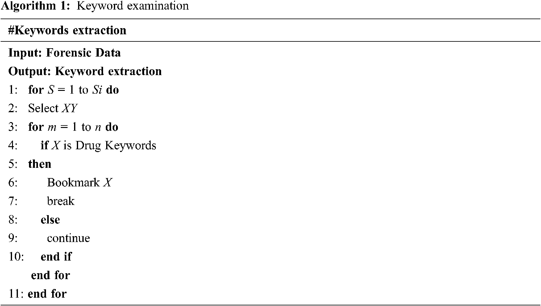
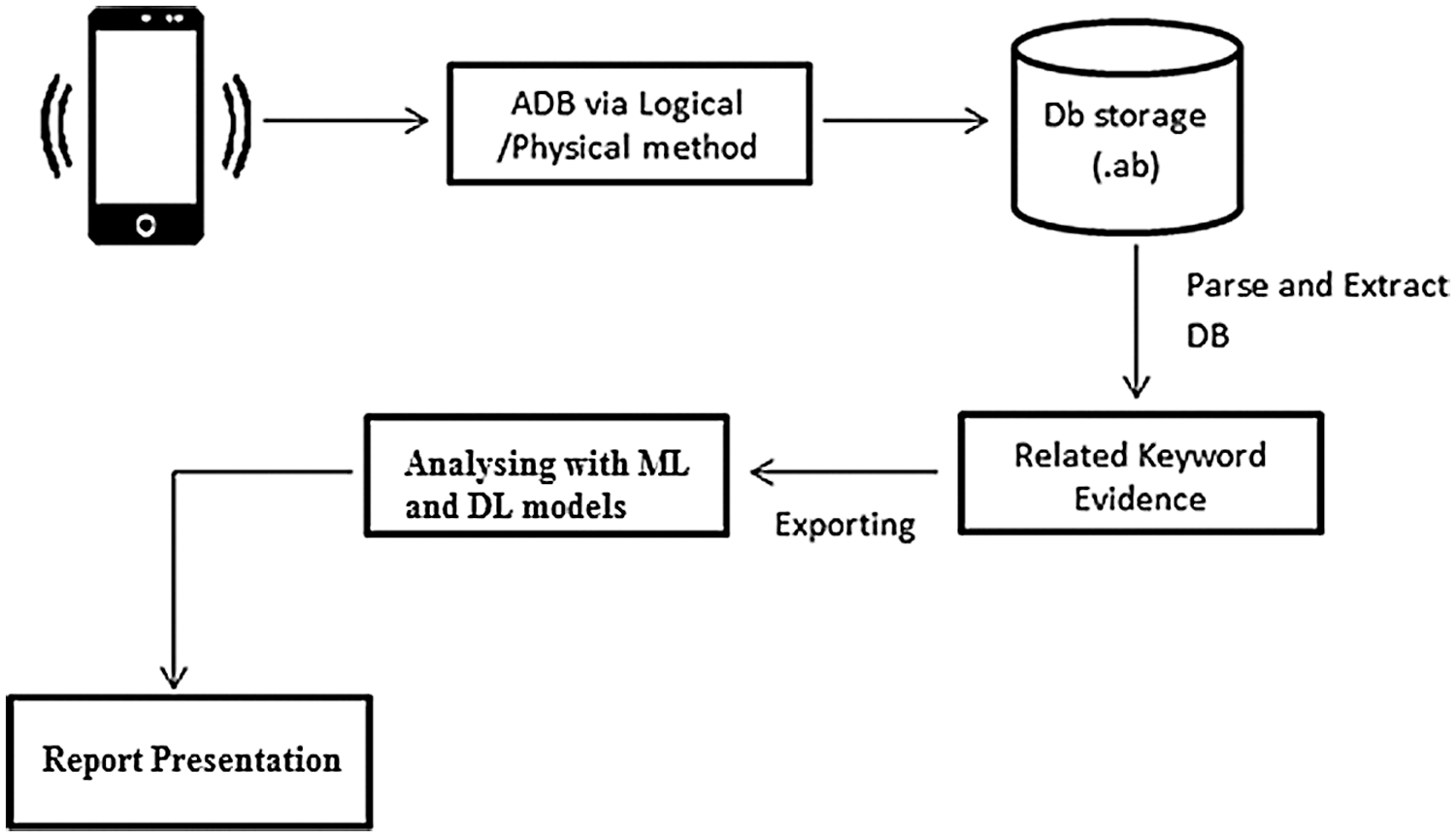
Figure 2: Working process of mobile device forensic
4.1 Considering ML Algorithms and its Evaluation Metrics
The experimental analysis is carried out utilizing Five Machine Learning models, namely; Logistic Regression (LR), Multinomial Naïve Bayes (MNB), Support Vector Machine (SVM), XGBoost, and LSTM. These algorithms are employed to classify the dataset, and best results are selected based on evaluation metrics. The authors divided the dataset into 70% of training data and 30% of testing data. In Machine Learning models, the feature extractions are to be made with Tokenization, Stemming, Tf-IDF, and many more techniques. In contrast, in Deep learning models, the feature extractions are made automatically. So, in our model, the baseline model is built with count vectorization, which helped convert the text document into small tokens. For text classification with the help of a count vectorizer, four types of ML models are used to analyse. TFIDF is used to extract the features from the text document to train and test the LR, MNB, SVM, and XGBoost. In the TFIDF method, the features of unigram, bigram, and trigram are extracted from corpus. The feature selection can also be used to eliminate noise and unnecessary symbols from the document.
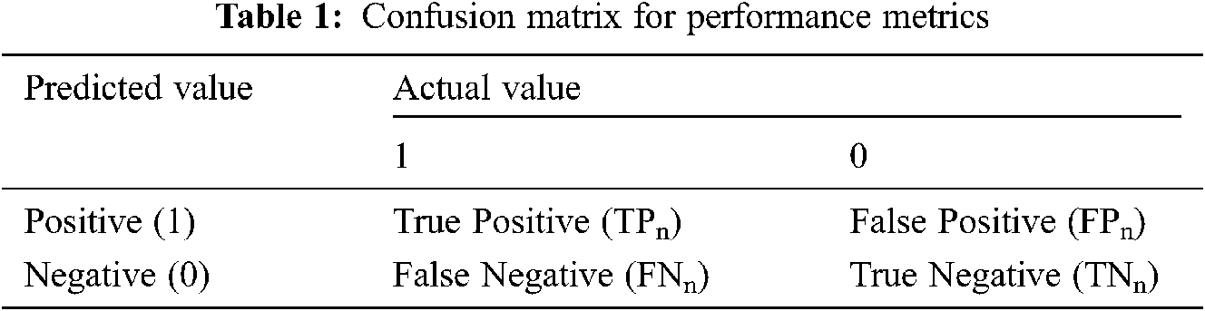
In this section, the techniques mentioned earlier produce performance metrics and confusion matrix in terms of Accuracy, Precision, F1 Score, and Recall. In any classification problem of machine learning, four combinations of predicted and actual values classification possibilities are employed as shown in Tab. 1. The TPn is True Positive, also known as sensitivity where observation and predicted values are positive, FNn is False Negative where observations are positive but predicted values are negative, FPn is False Positive, where a number of observations are negative but predicted value is positive, and TNn is True Negative also known as Specificity, where both observation and predicted values are negative.
Accuracy: As indicated in Eq. (1), the correctly identified dealer and client samples ratio to the total number of instances from the dataset are stated here.
Precision: The proportion of correctly classified samples to the total number of positively predicted or detected samples, are stated in Eq. (2).
Recall: It’s also known as True Positive Rate (TPR) or sensitivity. It’s the proportion of correct positive predictions/detection to the overall number of positives, as calculated in Eq. (3).
F1Score: Harmonic mean is used to calculate as given in Eq. (4).
From Eq. (1), we describe how performance measures are computed for all the classes n in the dataset that belongs to the SV set of suspiciousness values.
5 Anomaly Detection Based on ARIMA, SARIMA, and LSTM
After obtaining forensically extract data from mobile device, we analyze the frequency of smartphone illicit drug keywords. In this section, the authors propose a predictive analysis of illegal drug transfer based on a deep learning approach, namely ARIMA, SARIMA, and LSTM. This model is trained and tested with extracted data using a forensic toolkit, and attributes are filtered out based on our system to predict the future mode of transferring [16]. The Internet provides new opportunities to cybercriminals to enlarge their criminal activities in terms of illegitimate business, services, etc, and as a response, law enforcement is compelled to act. Ubiquitous data in terms of time series are transferred in our daily lives, ranging from stock markets, weather forecasting, messaging to retail sales, etc. Time series analysis comprises methods for analyzing data to extract statistical features of the time series data. Time series forecasting has a significant approach in predicting the future based on previously observed values. Machine learning and deep learning algorithms are used to indicate the values. So, this paper employs deep learning algorithms to analyze and predict the messages transferred over the years between drug dealers and clients. This prediction method is often plotted via line charts. Time series are used in pattern recognition, speech recognition, bitcoin prediction, weather, and earthquake prediction and applied to all temporal fields.
5.1 ARIMA (Autoregressive Integrated Moving Average)
ARIMA is termed Autoregressive Integrated Moving Average and it was introduced in 1960 by Box and Jenkins [17], who primarily utilized for time series forecasting. This model is described with three parameters; p, q, and d, where Auto Regressive of order belongs to p, Moving Average of order belongs to q, and d is the degree of difference. The final model is expressed as given in Eq. (5)
ARIMA is a linear method, from the past sample/ observation it can predict the future time series. It performs both properties of stationary and non-stationary series of data. The system will predict the series in terms of mean, variance, auto relation over time in a stationary property, whereas in non-stationary property, the data should be converted into the stationary property and it can be used for further analysis. From Eq. (5), let the actual data sample be
The extension of ARIMA is SARIMA which is termed as Seasonal Autoregressive Integrated Moving Average, and it is presented as [(p, q, d) (P, Q, D) S] where S is seasonal periods of time series, P, Q, and D are denoted as Autoregressive (AR), Differencing (D), and Moving Average (MA) respectively. The general equation for the model is given as follows:
In Eq. (6),
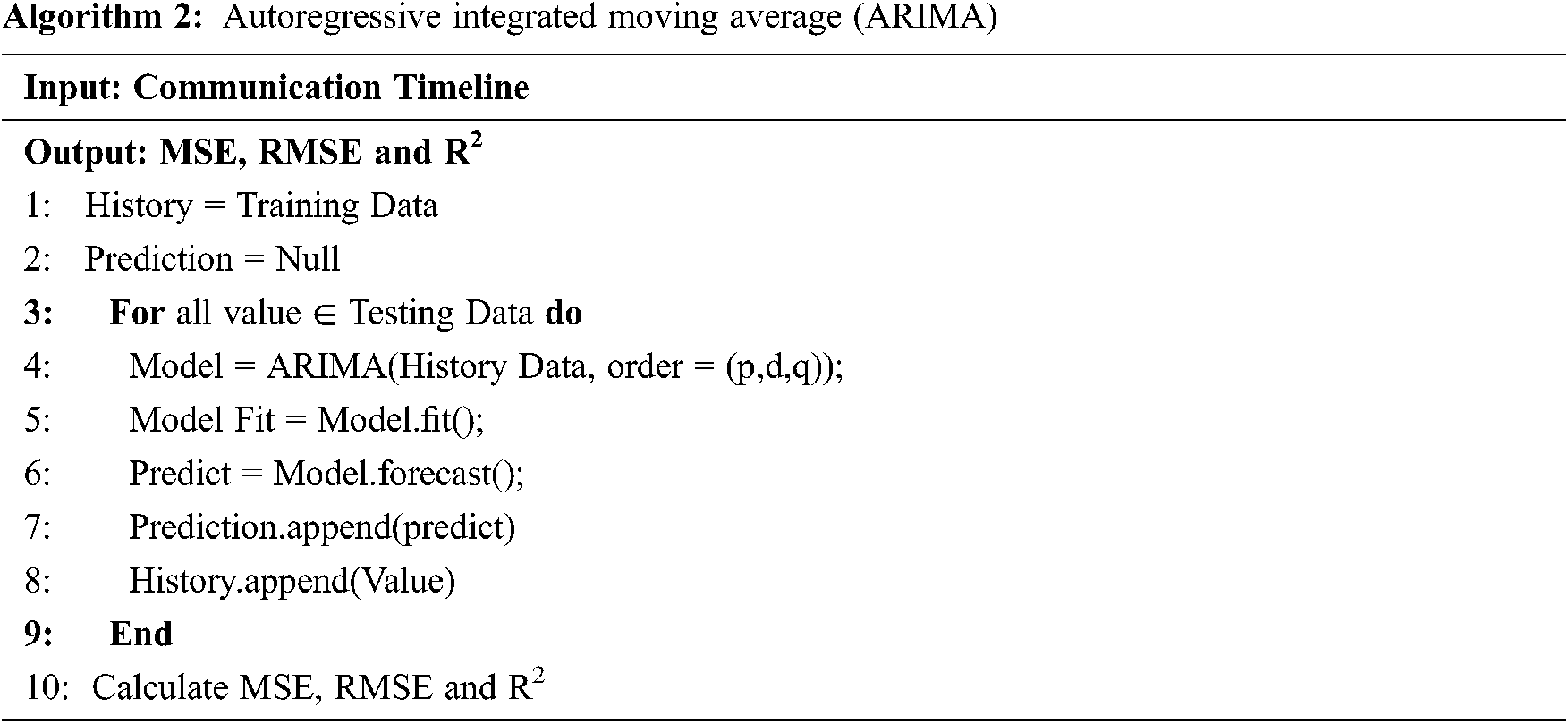
The ARIMA Algorithm listed in Algorithm 2 takes time-series as input data aids to build a forecast model. It calculates the MSE (Mean Squared Error), RMSE (Root Mean Squared Error), and R2 (R Squared) of the prediction model. An algorithm initially splits the data in the ratio of 70:30 and then uses training data at each iteration. As mentioned above, the notations p, d, and q are used to build the ARIMA model.
Here,
p is the lag observation of the training model (Lag order)
d is the differencing order
q is the order of moving average.
In this work, 1,1,3 for p, d, q order is used to test the data. More specifically, an ARIMA (1, 1, 3) represents that lag value which is set to 1 for autoregressive, the value 1 to time differencing for time series stationary, and finally, value 3 for moving average model.
After evaluating ML algorithms for mobile forensic data, the Long Short Team Memory (LSTM) based on neural network in Deep Learning is proposed to predict the event and time series prediction of crime data. To solve the vanishing and exploding gradients problem from Recurrent Neural Network (RNN), back propagation and Feed Forward neural network LSTM are introduced with three gates called forgot gate, input gate and output gate comprising into a memory cell. The working mechanism of LSTM is based on Eq. (8). Fig. 3 shows the LSTM structure where it represents the input gate, ot is output gate and ft is forgot gate with weight W, bias b, the activation function sigmoid
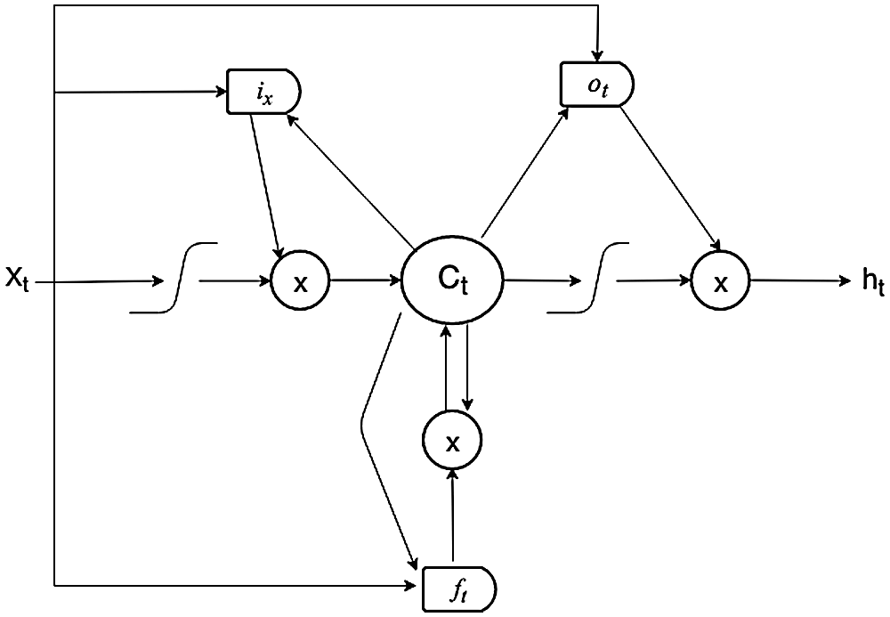
Figure 3: Structure of LSTM
i Forgot gate
An activation/sigmoid (
ii Input gate
The Input gate decides whether to add or update new information to the main memory cell between the values 0 and 1 where 0 represents not important and 1 means important. The sigmoid function will decide, which information needs to be added and updated which acts as a filtering from (ht-1) to Xt. Tanh function creates the vector values and is finally added to a cell state (8).
iii Output gate
The Output gate uses the sigmoid function to decide information from memory cell state and tanh function, after creating vector values which are used to scale the values between –1 to +1 as represented in ot (8). Finally, the result is multiplied to
Mobile forensic investigation is generally divided into four main phases: seizure, data acquisition, examination, and report presentation. Evidence collection and analysis are the primary tasks for examiners, which help in prosecution and defense. The functionalities of smartphone technologies are ever-advancing, resulting in the expansion of the drug trade market. Selling and buying of illicit drugs are taking place on social media through smartphones. Yet, keyword evidence search intends to analyze the acquired data for drug-related terms. The significant role of digital forensic examiners is to retrieve the past events from digital devices which are materializing the crime scene, as the suspect may delete, hide, modify and alter the digital evidence. So, it is necessary to maintain the integrity of retrieved data by faraday bag.
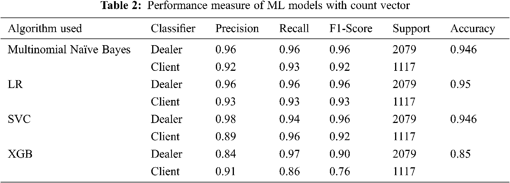
The performance measure for four classification algorithms is considered from supervised learning models as shown in Tab. 2. The metrics are calculated based on the count vector. From Tab. 3, the Logistic Regression algorithm manifests the highest accuracy of 95%, followed by MNB, SVM, and XGBoost with 94.6%, 94.6%, and 85%, respectively. Machine learning forensic is a developing technology that can recognize criminal activities’ behavioral and suspicious patterns to predict the time and place of crimes that occurred and those that could happen in the future. In this paper, the authors obtained all the possible data related to chats between drug dealers and clients’ from forensically sound data. Finally, the obtained results are analyzed by machine learning techniques to detect and identify the crime pattern. This paper aims to analyze and examine if machine learning techniques are successfully applied or not to obtain the desired results. This segment compares the performance measures of seven ML algorithms to identify the effective algorithm.
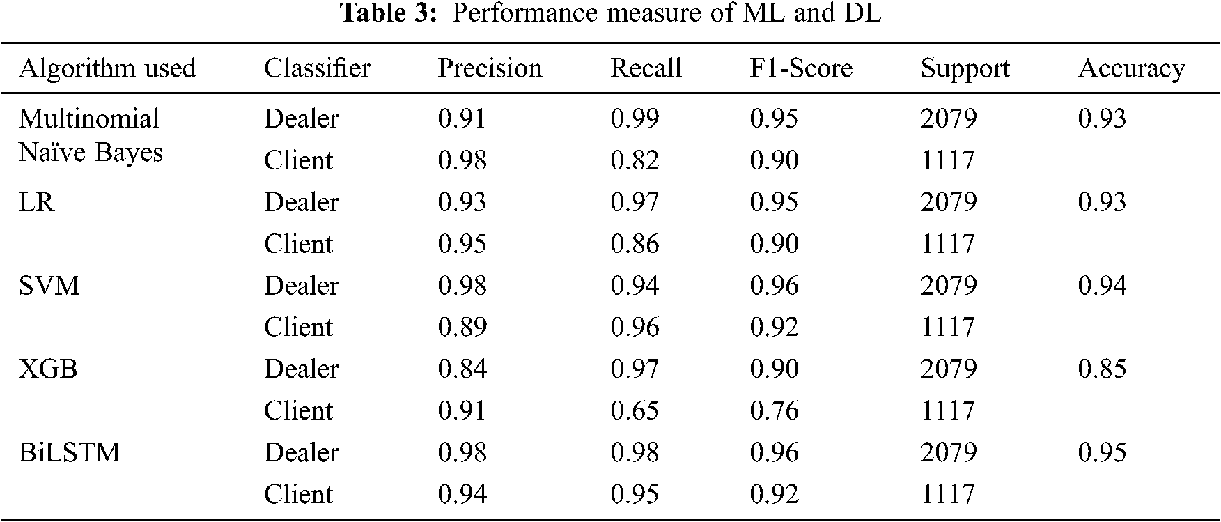
In this word embedding implementation, the maximum sequence length is 100, the maximum vocab size is 20000, and the number of glove dimensions is 50d with a validation split of 0.3. From Tab. 3, the performance measure indicates that BiLSTM reached the highest accuracy of 95% with word embedding technique followed by SVM, LR and MNB with the rate of 94%, 93% and 93% whereas, XGBoost reached lowest accuracy of 85%. This indicates that 30% of the training data will be utilized to validate the model during the training phase. The batch size is 64, and the model is trained with 10 data points. Machine learning forensic is a developing technique that can recognize the behavioral and suspicious patterns of criminal activities to predict the time and place of crimes and those that could happen in the future. In this paper, the authors obtained all the possible data related to chats between drug dealers and clients from mobile device and forensically sound data. Finally, the obtained results are analyzed by machine learning techniques to detect and identify the crime pattern. This paper aims at analyzing and examining if machine learning techniques are successfully applied or not to obtain the desired results.
The accuracy of both the systems has been compared with the count vector and TFIDF method. From Fig. 4, we can understand that accuracy of LR model has reached 95% with the count vector, whereas; the BiLSTM model has also got the same accuracy of 95%.
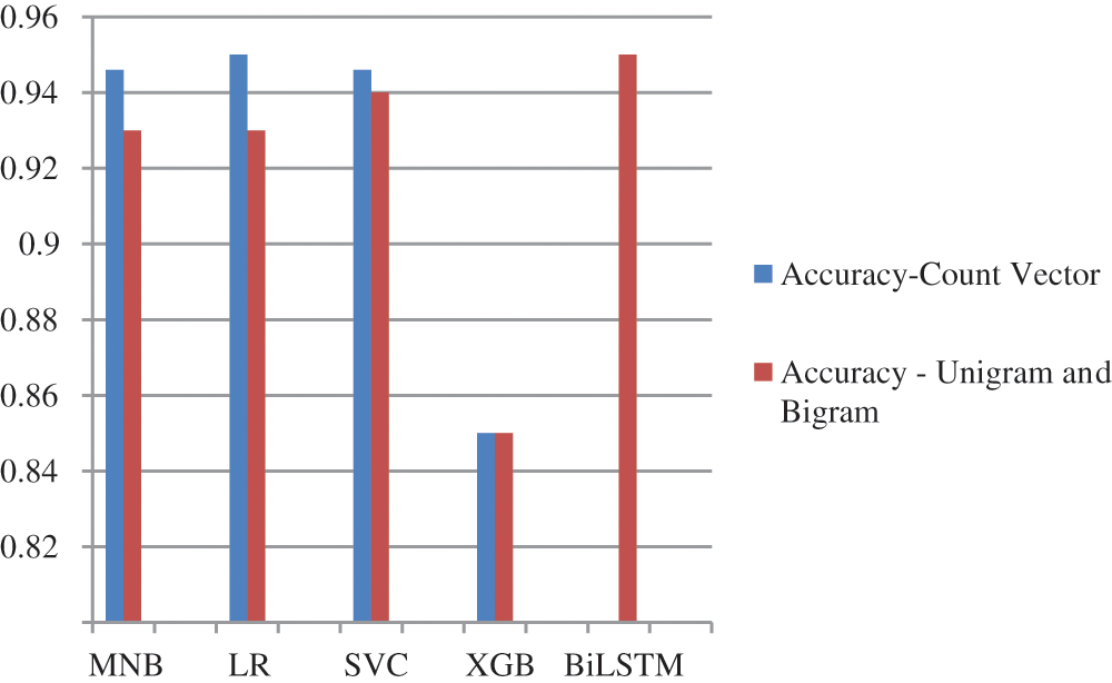
Figure 4: Comparison of accuracy with count vector and TFIDF
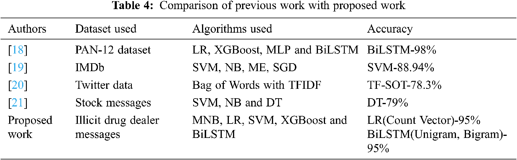
The comparison of accuracy has been made with other studies similar to classification problems with various datasets. Tab. 4 represents the work previously made by other researchers. Ngejane et al. used the PAN-12 dataset to identify the online sexual chat logs using four algorithms, in which BiLSMT acquired 98% of accuracy. Tripathy et al. used the Internet Movie Database (IMDb) and analyzed them with four algorithms, namely; Support Vector Machine (SVM), Naïve Bayes (NB), Maximum Entropy (ME) and Stochastic Gradient Descent (SGD) models with the highest accuracy of 88.94% for SVM algorithm. Similarly, the author Niu used Twitter data and analyzed them using BOW (Bag of Words) and TFIDF. Finally, the researchers (Luo et al.) used stock messages for text classification with three algorithms namely; SVM, NB and Decision Tree (DT), and reached the highest accuracy of 79% for DT. The Mean Squared Error, Mean absolute error, Root Mean Squared Error, and R-Squared or Coefficient of determination metrics are used to evaluate the performance of the model. The Mean Squared Error represents the average of the squared difference between original and predicted values in data as represented in Eq. (9). The Root Mean Squared Error is the square of MSE. The formula is given in Eq. (10) and R squared or R2 is the proportion of variance in the dependant variables are predictable from the independent variables which is represented in Eq. (11).
Time series modeling is an exciting area where applications like sales forecasting, stock market forecasting and many more predict the future. This study aims to provide a new application in which time series can be used and build a model that helps predict the future values of time series. So, in this paper authors attempted to analyze the drug dealer’s transaction communication. First, messages between dealers and clients are retrieved from a mobile device using forensic software. After recovering, the chats are imported in comma-separated value (CSV) format with all the necessary details such as time, data, messages, etc. Generally, time series algorithms work with time series, which are gathered at regular intervals. In this part, the ARIMA, SARIMA, and LSTM time series algorithms are used to forecast the dealers and clients communication. Tab. 5 and Figs. 5–7 provide the output for ARIMA, SARIMA, and LSTM prediction, and in the ARIMA algorithm, the authors have used 1,1,3 order.
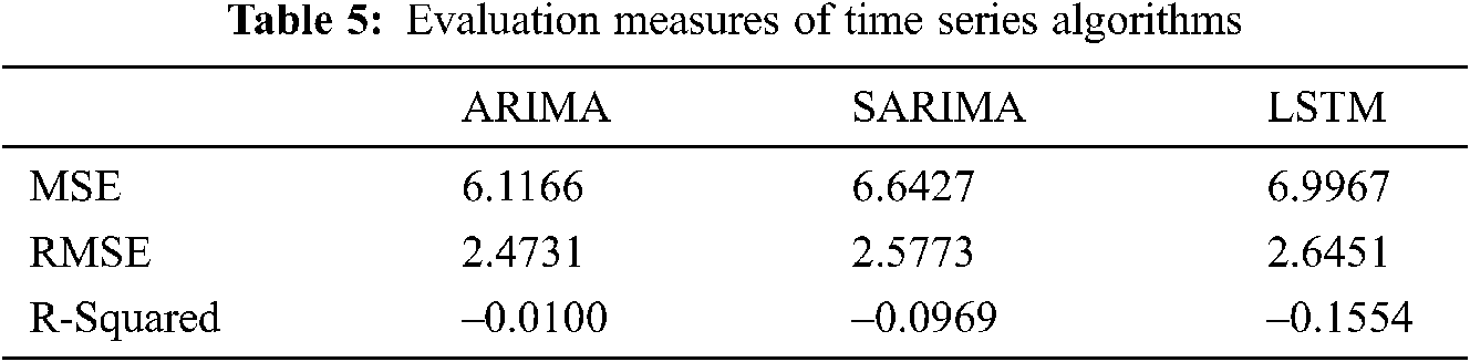
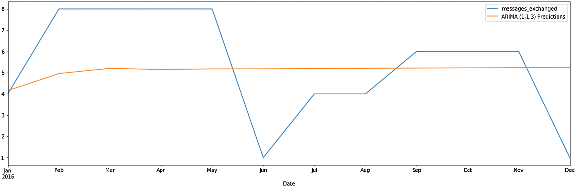
Figure 5: ARIMA prediction
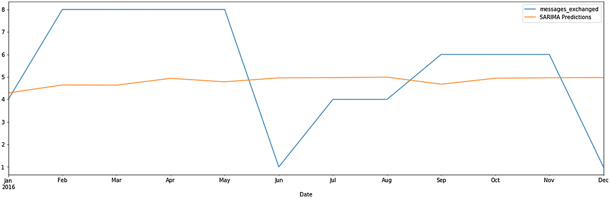
Figure 6: SARIMA prediction
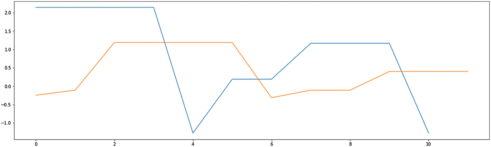
Figure 7: LSTM prediction
This research focused on investigating the suspicious patterns of drug dealing digital prints from mobile devices and social networks by using forensic and ML techniques identified as incrementing evidence by tracing. ML algorithms aim to investigate footprints of call logs to analyze the evidence to determine the criminal activities. The collected dataset contained all relevant digital footprints related to illicit drug dealers’ identities and then they were fed to seven ML algorithms. Several evaluation metrics were used to compare the performance of each algorithm. The results of the experiments revealed that LR and SVM generated the best results. The final part of the paper compares the accuracy of ARIMA, SARIMA, and LSTM as represented for time series analysis. These techniques are implemented on the drug dealers dataset, and results showed that the ARIMA model worked better than the other two models. The authors intend to extend the work with More Machine Learning (ML) and Deep Learning (DL) methods for real time Mobile Device Forensic cases. So, the author aims to develop an independent, stand-alone system for examining mobile forensic cases incorporated with AI (Artificial Intelligence) System. These datasets can then be used to build respective ML and DL models for predicting new cases of the same pattern. Future work will help to identify the criminals as early as possible during an investigation.
Funding Statement: The authors received no specific funding for this study.
Conflicts of Interest: The authors declare that they have no conflicts of interest to report regarding the present study.
1. R. Tamma, O. Skulkin, H. Mahalik and S. Bommisetty, Pratical Mobile Forensics, 3rded., Birmingham, UK, 2016. [Online]. Available:https://pre-uneplive.unep.org/redesign/media/assets/images/Practical%20Mobile%20Forensics.pdf. [Google Scholar]
2. M. T. Britz, Computer Forensics and Cyber Crime an Introduction, 3rded., Pearson, 2013. [Online]. Available: http://index-of.es/Varios2/Computer%20Forensics%20and%20Cyber%20Crime%20An%20Introduction.pdf. [Google Scholar]
3. E. Casey and B. Turnbull, “Digital evidence on mobile devices,” in Digital Evidence and Computer Crime, 3rded., Elsevier, pp. 1–44, 2011. [Online]. Available:https://booksite.elsevier.com/samplechapters/9780123742681/Front_Matter.pdf [Google Scholar]
4. D. Quick and K. R. Choo, “Impacts of increasing volume of digital forensic data: A survey and future research challenges,” Digital Investigation, vol. 11, no. 4, pp. 273–294, 2014. [Google Scholar]
5. X. Yang and J. Luo, “Tracking illicit drug dealing and abuse on Instagram using multimodal analysis,” ACM Transactions on Intelligent System and Technology, vol. 8, no. 4, pp. 1–15, 2017. [Google Scholar]
6. F. Amato, G. Cozzolino, V. Moscato and F. Moscato, “Analyse digital forensic evidences through a semantic-based methodology and NLP techniques,” Future Generation Computer Systems, vol. 98, pp. 297–307, 2019. [Google Scholar]
7. N. M. Karie, V. R. Kebande and H. S. Venter, “Deep learning cognitive computing techniques into cyber forensics,” Forensic Science International: Synergy, vol. 1, pp. 61–67, 2019. [Google Scholar]
8. D. Walnycky, I. Baggili, A. Marrington, J. Moore and F. Breitinger, “Network and device forensic analysis of Android social-messaging applications,” Digital Investigation, vol. 14, no. 3, pp. S77–S84, 2015. [Google Scholar]
9. G. Horsman, “Formalising investigative decision making in digital forensics: Proposing the digital evidence reporting and decision support (DERDS) framework,” Digital Investigation, vol. 28, no. 1, pp. 146–151, 2019. [Google Scholar]
10. H. Arshad, A. Jantan, G. Keng and A. Sahar, “A multilayered semantic framework for integrated forensic acquisition on social media,” Digital Investigation, vol. 29, no. 11, pp. 147–158, 2019. [Google Scholar]
11. M. Nicoletti and M. Bernaschi, “Forensic analysis of Microsoft Skype for Business,” Digital Investigation, vol. 29, no. 1, pp. 159–179, 2019. [Google Scholar]
12. R. M. A. Mohammad and M. Alqahtani, “A comparison of machine learning techniques for file system forensics analysis,” Journal of Information Security and Applications, vol. 46, pp. 53–61, 2019. [Google Scholar]
13. A. Cohen, N. Nissim, L. Rokach and Y. Elovici, “SFEM: Structural feature extraction methodology for the detection of malicious office documents using machine learning methods,” Expert System Application, vol. 63, no. 2-3, pp. 324–343, 2016. [Google Scholar]
14. H. Studiawan, C. Payne and F. Sohel, “Graph clustering and anomaly detection of access control log for forensic purposes,” Digital Investigation, vol. 21, no. 1, pp. 76–87, 2017. [Google Scholar]
15. A. Dey, “Machine learning algorithms: A review,” International Journal of Computer Science and Information Technologies, vol. 7, no. 3, pp. 1174–1179, 2016. [Google Scholar]
16. G. M. Jones and S. G. Winster, “Prediction of novel coronavirus (nCOVID-19) propagation based on SEIR, ARIMA and Prophet model” In: P. K.Khosla, M.Mittal, D.Sharma, L. M.Goyal.(edsPredictive and Preventive Measures for Covid-19 Pandemic, Algorithm, pp. 189–208, 2021. [Google Scholar]
17. A. K. Shrivastav and Ekata, “Applicability of box jenkins ARIMA model in crime forecasting: A case study of counterfeiting in Gujarat state,” International Journal of Advanced Research in Computer Engineering & Technology, vol. 1, no. 4, pp. 494–497, 2012. [Google Scholar]
18. C. H. Ngejane, J. H. P. Eloff, T. J. Sefara and V. N. Marivate, “Digital forensics supported by machine learning for the detection of online sexual predatory chats,” Forensic Science International: Digital Investigation, vol. 36, pp. 1–11, 2021. [Google Scholar]
19. A. Tripathy, A. Agrawal and S. K. Rath, “Classification of sentiment reviews using N-gram machine learning approach classification of sentiment reviews using n-gram machine learning approach,” Expert System Application, vol. 57, no. 2, pp. 117–126, 2016. [Google Scholar]
20. T. Niu, S. Zhu, L. Pang and A. Saddik, “Sentiment analysis on multi-view social data,” In: Proceedings of the International Conference on Multimedia Modeling, Springer, Miami, FL, USA, 4–6 1 2016, pp. 15–27, 2016 [Google Scholar]
21. B. Luo, J. Zeng and J. Duan, “Emotion space model for classifying opinions in stock message board,” Expert System Applications: An International Journal, vol. 44, no. 3, pp. 138–1446, 2016. [Google Scholar]
 | This work is licensed under a Creative Commons Attribution 4.0 International License, which permits unrestricted use, distribution, and reproduction in any medium, provided the original work is properly cited. |