Intelligent Automation & Soft Computing DOI:10.32604/iasc.2022.022860
Article

Optimized Compressive Sensing Based ECG Signal Compression and Reconstruction

Ishani Mishra1,* and Sanjay Jain2

1Department of ECE, New Horizon College of Engineering, Bengaluru, 560103, India
2Department of ECE, CMR Institute of Technology, Bangalore, 560037, India
*Corresponding Author: Ishani Mishra. Email: ishannimishra2021@gmail.com
Received: 20 August 2021; Accepted: 11 October 2021

Abstract: In wireless body sensor network (WBSN), the set of electrocardiograms (ECG) data which is collected from sensor nodes and transmitted to the server remotely supports the experts to monitor the health of a patient. However, due to the size of the ECG data, the performance of the signal compression and reconstruction is degraded. For efficient wireless transmission of ECG data, compressive sensing (CS) frame work plays significant role recently in WBSN. So, this work focuses to present CS for ECG signal compression and reconstruction. Although CS minimizes mean square error (MSE), compression rate and reconstruction probability of the CS is further to be improved. In this paper, we provide an efficient compressive sensing framework which strives to improve the reconstruction process, by adjusting the sensing matrix during the compression phase using the rain optimization algorithm (ROA). With the optimal sensing matrix, the compressed signal is reconstructed using Step Size optimized Sparsity Adaptive Matching Pursuit algorithm (SAMP). The results of this work demonstrate that the optimised CS framework achieves a higher compression rate and probability of reconstruction than the standard CS framework.

Keywords: Wireless body sensor network (WBSN); optimized compressive sensing; step size optimized sparsity adaptive matching pursuit algorithm (SAMP); rain optimization algorithm (ROA)

1  Introduction

The term “WBSN” refers to a networking technology that connects several sensor nodes within or on the human body It very well may be utilized in the use of medical care for persistent monitoring of patients [1,2]. The data is collected via a few sensor nodes that are either embedded or surface mounted on the human body and transmitted to smart devices such as cell phones or tablets. The information obtained by sensors on the smart gadget can be remotely transferred to specialists or doctors located anywhere in the globe via the Internet, who can screen, analyse, or converse with the patient remotely as the wearable sensors are attached to and move with the patients. In this way, WBSN gives mobile monitoring of patients, where patients need not be at or close to clinics for their ceaseless health observing.

WBSN can sense numerous physiological signals like electromyogram (EMG), electroencephalogram (EEG), electrocardiogram (ECG), internal temperature, pulse and interestingly, the patients’ breathing or movement. Among them, ECG is critical because it enables the analysis of cardiovascular diseases, which are the leading cause of death, according to a WHO report [3]. Given the significance of ECG signal assessment from the health point of view, this work focuses exclusively on ECG signals. Thus, procurement, handling, storing, transmission, joining and recovery of ECG signals assume a significant part in WBSN [4,5]. In this way, ECG compression is a significant factor in current medical services frameworks to lessen the expense and increment the effectiveness of signal processing frameworks. It is alluring to lessen the component of ECG signals while safeguarding the significant diagnostic data in recorded ECGs [6].

A few algorithms have been presented over the decades for ECG signal compression and reconstruction. Compressed Sensing (CS) is a developing structure in contemporary signal processing that enables the capture and preparation of insufficient signals as well as signals with sparse representation in some appropriate premise [7]. CS suggests that limited dimensional signals consisting sparse or compressible representation can be recuperated from a little linear set, non-adaptive estimations. This outcome shows that it is feasible to test the sparse signals by taking far less estimations than regular Nyquist sampling rate. As a result, recovery of signal is typically accomplished by utilizing highly nonlinear and complex techniques.

1.1 Problem Statement

In terms of sensor energy consumption, data transmission rate is seen as a critical factor in determining how much energy is consumed by WBSN devices. A great deal of ongoing investigates are basically centred on decreasing the number of data transmissions in WBSN. CS is primarily concerned with three perspectives: signal sparse representation, view of the measurement matrix, and reconstruction procedure. To enhance the performance of sparse reconstruction in CS, sensing matrix is to be optimized in the phase of compression.

1.2 Contribution

•   We propose a technique to improve the reconstruction process by optimizing the CS matrix using rain optimization algorithm (ROA). Using this algorithm, optimized CS matrix is chosen. Mean square error (MSE) is considered as an objective function. The CS matrix with minimum error is chosen as an optimal matrix.

•   Then, the compressed signal is reconstructed by applying step size optimized sparsity adaptive matching pursuit algorithm.

Remaining sections of the manuscript are sorted as follows. Compressive sensing for ECG signals based recent research works are survived in Section 2. Section 3 proposes optimized compressive sensing, namely ROA based data compression and step size optimized sparsity adaptive matching pursuit algorithm for reconstruction. Results of the proposed scheme are discussed in Section 4. The conclusion of the research work is described in Section 5.

2  Related Works

Recent Compressive sensing based EGC signal compression and reconstruction works are reviewed in this section. Rezaii et al. [8] have presented the selection of efficient sparsity order for the compression and denoising of ECG signal in compressive sensing system. Aim of the authors was to attain the better compression ratio than the convention ECG compression schemes. So, they have proposed optimum sparsity order selection method through which the sparsity order was determined by reducing the error of reconstruction. Besides, the authors have proved that the raised Cosine kernel-based basis matrix has better efficiency than the Gaussian basis matrices. The article’s findings indicated that the unique approach resulted in a higher compression ratio.

Ansari et al. [9] have aimed to enhance the reconstruction of ECG based on compressive sensing in wireless body area network. To do this, the authors have proposed weighted non-convex minimization based EGClet that was abbreviated as WNC-EGClet. They highlighted three major innovations in their approach: non-convex minimization for ECG reconstruction using Compressive sensing, weighted sparsity on wavelet coefficients of ECG signals to reduce reconstruction error, and wavelet transform learning for ECG signals. Simulation results of the article showed that the novel WNC-ECGlet outperformed previous ECG reconstruction based on compressive sensing.

Polanía et al. [10] had goal to decrease the communication burden and energy consumption in compressive sensing. They accomplished this by introducing restricted Boltzmann machines, abbreviated as RBMs. By reducing the number of necessary measurements, the authors accomplished effective reconstruction using RBMs. Besides, the probability distribution of the sparsity pattern of ECG signals was modelled using RBMs. Based on the approach, the higher-order statistical dependencies between the EGC sparse coefficients. The technique elucidates the higher-order statistical relationships between the EGC sparse coefficients and achieved better reconstruction accuracy.

Abhishek et al. [11] sought to improve the quality of reconstruction by reducing number of samples in compressive sensing. To achieve this goal, the authors have proposed biorthogonal wavelet filters. Contrasted to orthogonal wavelets, Biorthogonal wavelets have more advantages like linear phase. Using this wavelet filter, double exponential wavelet 1 was applied in ECG reconstruction based on compressive sensing. The proposed strategy resulted in a lower energy consumption for compressive sensing than the current ECG reconstruction.

Jahanshahi et al. [12] had the objective that to monitor the multi-channel ECG signals efficiently in wireless body sensor network. The authors have enhanced the performance of compression by extracting the spatio-temporal correlations of the multi-channel ECG signals using Kronecker sparsifying bases. Besides data acquisition and reconstruction was achieved by presenting compressive sensing with the low-rank constraint. Alternating direction method of multipliers (ADMM) was designed for reconstruction of multi-channel ECG signals. Simulation results of the article showed that the proposed scheme achieved better accuracy and low computational complexity.

Rakshit et al. [13] had aimed to recover the signal based on beat kind dictionary and non-uniform random sensing matrix. Thus, the authors provided a strategy to ECG-compressive sensing based on an effective beat type dictionary. This beat type dictionary provided high-quality signal reconstruction without the training phase for each ECG record. By presenting this proposed scheme, they have achieved better compression ratio and signal-to-noise ratio.

Kumar et al. [14] had the goal to reduce the energy consumption while transmitting the multi-channel ECG data in wireless body area networks. To accomplish this, the authors presented a method for multi-channel ECG compression based on block sparsity. Using the proposed scheme, multi-scale data and spatiotemporal correlation of multi-channel ECG data in the domain of wavelet were exploited. The article’s simulation results indicated that the proposed method consumed less energy than standard compressive schemes.

3  Optimized Compressive Sensing Technique for ECG Signal Compression and Reconstruction

The ECG data sensed by the body sensors are collected by a device like mobile phone as shown in Fig. 1 is the overall block diagram of the optimized compressive sensing technique. As shown in the figure, the ECG data sensed by the body sensors are collected by a device like mobile phone. As illustrated in the image, a device such as a mobile phone collects the ECG data sensed by the body sensors.

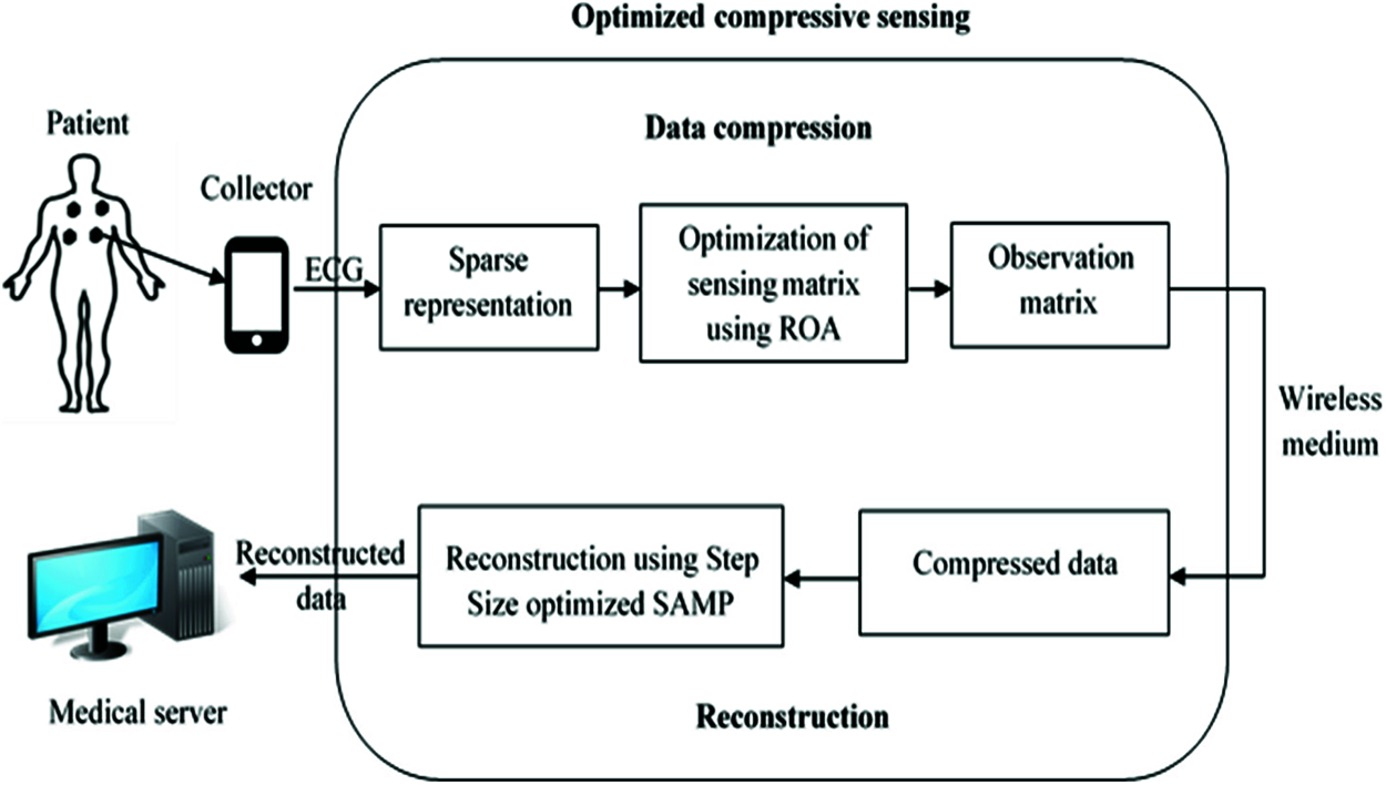
Figure 1: The block diagram of the optimized CS

3.1 Overview

The input data or signal is represented as a sparse signal and compressed by multiplying it by the observation matrix. To enhance the performance of the data compression, the sensing matrix must be optimized to achieve this. So, for optimization of sensing matrix, rain optimization algorithm (ROA) is presented. Then, at the medical server, with the observation matrix, the original signal is reconstructed using step size optimized SAMP algorithm. The suggested reconstruction approach employs a smaller step size to improve the performance of the SAMP algorithm.

3.2 Compressive Sensing

Using a predetermined matrix, compressive sensing is used to convert data from a high-dimensional space to a low-dimensional space. Besides, this technique is applied to compress the signal and to reconstruct the compressed signal. Compressive sensing consists of three major stages: sparse representation, generating the observation matrix, and signal reconstruction.

As the original signal is not sparse, it must be transformed and represented in sparse domain. In compressive sensing, sparsity means that the signal has k degree of non-zero value in transform domain.

As per the function of sparse transform, the input signal x is considered to have ϕ sparse representation. So, the input signal can be represented as Eq. (1)

x=ϕψ (1)

where, ψ the transform matrix and ϕ denotes the sparse representation of signal x.

The compressed samples of the signal x are obtained using the observation matrix as defined in Eq. (2)

y=φx (2)

where, φ denotes the measurement matrix which is projected on signal x.

The Eq. (2) can be written as follows,

y=φψϕ=Sϕ (3)

where, S = φψ denotes the sensing matrix

Emmanuel C and S and Terence Tao established that the measurement matrix used to reconstruct the compressed signal must meet the Restricted Isometry Property (RIP) [15]. If the sparse transform and measurement matrix satisfy the incoherence criterion, the chance of reconstructing y is high. If S satisfies the RIP condition, φ is reconstructed by attaining the solution defined in Eq. (4).

ϕ^=arg min‖ϕ‖0s.t.y=Sϕ (4)

where, ϕ^ denotes the reconstructed sparse coefficient and ‖‖0 denotes the l0 norm. The Eq. (4) is the greedy reconstruction algorithm.

As the computational complexity of compressive sensing is very high especially in reconstruction, the performance of the compressive sensing is to be enhanced. As a result, we will concentrate on data compression and reconstruction which is further enhanced by refining the sensor matrix using the ROA method. It also results in an increase in the reconstruction performance and as next process, we present step size varied SAMP reconstruction algorithm which also enhances the performances of reconstruction further. Nevertheless, we present step size varied SAMP reconstruction algorithm which also enhances the performances of reconstruction further. The next sections discuss compressive sensing’s optimum data compression and reconstruction.

3.3 Data Compression with ROA Based Compressive Sensing

As shown in Fig. 1, the sensed ECG signals from the human body are collected by the monitoring device which forwards the data to the medical server. At transmitter side, the data or signal is compressed with compressive sensing. Prior to compression, the input data is converted using the sparse transform specified in the equation. Following sparse representation, data samples are compressed using the sensing matrix and sparse transform specified in Eq. (4). After sparse representation, the data samples are compressed using sensing matrix and sparse transform. To improve data compression performance, the sensing matrix (S) is tuned using the rain optimization algorithm (ROA).

The rain optimization algorithm (ROA) imitates the behaviour of rain drops. Raindrops normally stream down along a slant from a pinnacle at that point structure the waterways and consistently move to the lowest land points or void out into the ocean. The raindrops follow breaks and overlays in the land as they stream downhill. As the water flows downhill, it may become trapped in the potholes and features of the local optimum lake. Finally, the majority of streams reach the global ideal level and empty out into the ocean. The way the proposed method evolves from speculation to ideal is akin to a raindrop falling from a mountain to the ocean level in a hilly terrain due to gravity. As consistently raindrop will always choose the path with the more extreme slant, ROA reproduces this propensity and uses the slope of the target capacity to decide the solution that is better than an estimate.

To track down the deepest valley and afterward reach to the ocean level known as global optimal, a population of raindrops is created arbitrarily at initial iteration. The positions of the neighbour-points of each drop are compared with the position of drop before the drop moves towards the neighbour point possessing the least position. This development proceeds until the drop arrives at the valley. However long every one of the drops are streaming down from an upper to a lower position, regardless of whether there are puddles on the drops‟ route to the valley, they can in any case flood and rise out of the puddles to continue to move towards the valley by a fitting component performed by the ROA algorithm.

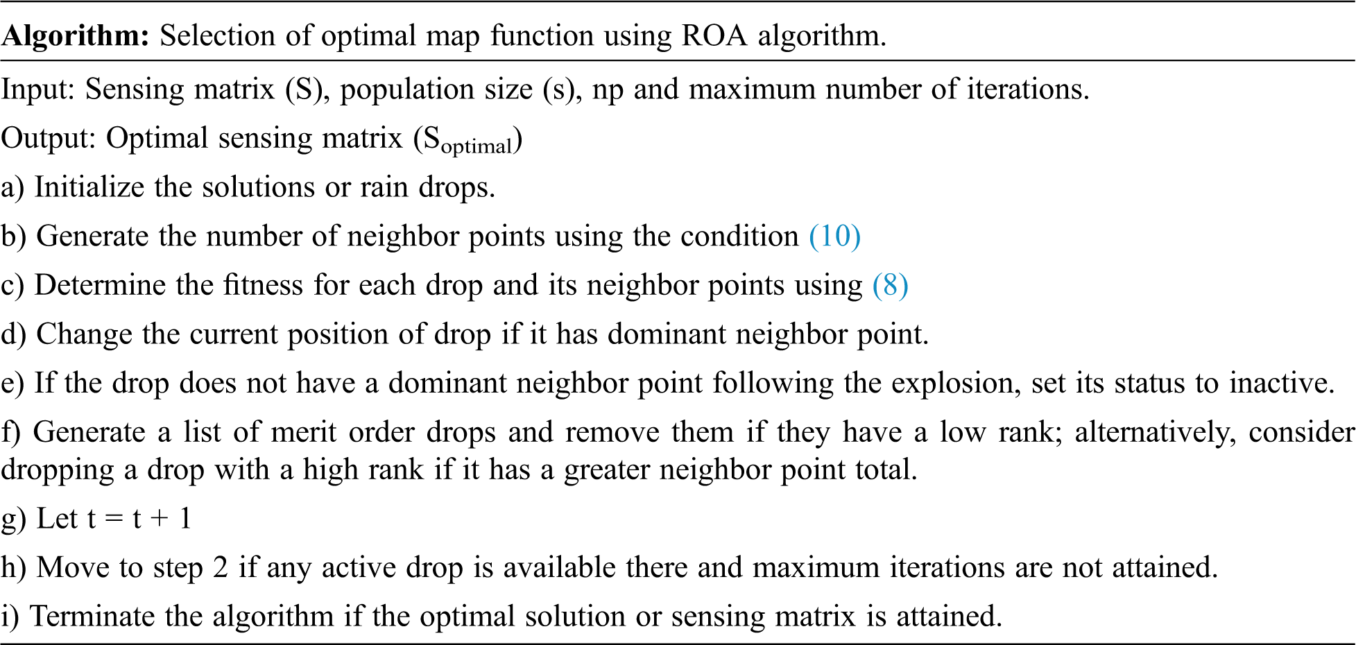
The process for optimizing sensing matrix (S) using ROA algorithm is described as follows:

3.3.1 Initialization

Each particle or raindrop in a population denotes the partial solution in this procedure. The optimal sensing matrix is the overall solution to this technique (S). The initialization of ith drop is defined as follows,

Di={yi,1,yi,2,yi,3,…,⁡yi,j}i∈[1,2,3,…,s] (5)

where, s denotes the size of the population, j denotes the number of optimization variables and yi,j denotes the variables of optimization problem. For this work, the variable can be defined as follows,

yi,j={S}i,j (6)

where, S denotes the sensing matrix.

Rainfall manages raindrops during the process of optimization. It is created by uniform random distribution function and subject to subject to constraints as given in Eq. (7).

yi,j=U(upj,lowj) (7)

where, U denotes the uniform distribution function, upj and lowj denote the upper and lower limits of yj.

3.3.2 Fitness Calculation

After initialization, fitness or objective function is recursively treated for optimal solution. To select the optimal sensing matrix, the solution should satisfy the following fitness function,

Fiti=Min(MSE(i)) (8)

where, MSE (i) denotes the mean square error of the ith solution and it can be defined as follows,

MSE(i)=1n∑n(x[n]−x^[n])2 (9)

where, n denotes the time index, x[n] denotes the input signal and x^[n] denotes the recovered signal.

According to Eq. (8), the optimal solution is obtained for the minimum value of MSE. Otherwise, the solution is recursively updated until finding the optimal solution. Through the following phases the solution is updated.

3.3.3 Update the Solution

As the raindrop (D) is defined as a point in N dimensional space, the domain which has the radius vector (r) places around the point is known as the neighbourhood. The neighbourhood can be updated when the changes occur in the value of raindrop.

During the process of optimization, a point in the neighbourhood of drop can be generated randomly. The ith drop’s neighbourhood point q is denoted as NPqi. Using the following condition, neighbour point of the drop is generated.

i=1,2,3,…,s‖u^p∗(Di−NPqi)‖≤‖u^p∗r‖forq=1,2,3,…,npp=1,2,3,…,z (10)

where, np denotes the number of neighbour points, u^p denotes the unit vector of the pth dimension. r denotes the size of the neighbourhood in terms of real positive vector and can be defined as follows,

r=f(itr)∗rinitial (11)

where, rinitial denotes the initial size of the neighbourhood and f(itr) denoted as a function used to adapt the size of the neighbourhood within iterations.

Dominant drop: The dominant neighbour point ( NPdi ) is one of the points chosen from the drop’s (Di) neighbour point. It should satisfy the following condition,

Fit(Di)>Fit(NPdi)

Fit(NPqi)>Fit(NPdi)

Active drop: The drop is considered as active drop if it has dominant neighbour point.

Inactive drop: The drop is considered as inactive drop if it does not have dominant neighbour point.

Process of explosion: If the drop has no sufficient neighbour points or it could not continue the search process to attain the optimal minimum, the explosion process is initiated to solve this condition of the drop. Using Eq. (12), the number of neighbour points can be created in this explosion process.

npE=be×np×ce (12)

where, npE denotes the number of neighbour points created in the process of explosion, np denotes the number of neighbour points without the process of explosion and ce denotes the counter of explosion, be denotes the explosion base (indicating the explosion range).

Rank of raindrop: For each rain drop, rank (R) is calculated using Eq. (15) in every iteration. This rank is used in the merit order list.

V1ti=Fit(Di)|attthiteration−Fit(Di)|atfirstiteration (13)

V2ti=Fit(Di)|attthiteration (14)

Rti=order(V1ti)∗ϕ1+order(V2ti)∗ϕ2 (15)

where, V1ti denotes the difference between the fitness function of drop Di at first iteration and tth iteration, V2ti denotes the fitness function of drop Di at tth iteration, order(V1ti) and order(V2ti) denote the orders of V1 and V2 at tth iteration when they are arranged in the form of ascending order, ϕ1 and ϕ2 denote the weighting coefficients that are assumed as 0.5 and Rti denotes the rank of rain drop at tth iteration.

List of merit order: For every iteration, ranks of the rain drops are arranged in ascending order. From the list, each low-ranking drop can be removed and some drops can be given significant rights. The drop with minimum fitness function is considered as the optimal solution.

3.3.4 Termination

The above process is repeated until finding the solution with the minimum fitness function. Otherwise, the algorithm is terminated.

After attaining the optimal sensing matrix (Soptimal), the compressed sample is calculated as follows,

y=Soptimal∅ (16)

From the compressed output, the signal is reconstructed using Step Size optimized SAMP. The following section explains the reconstruction algorithm.

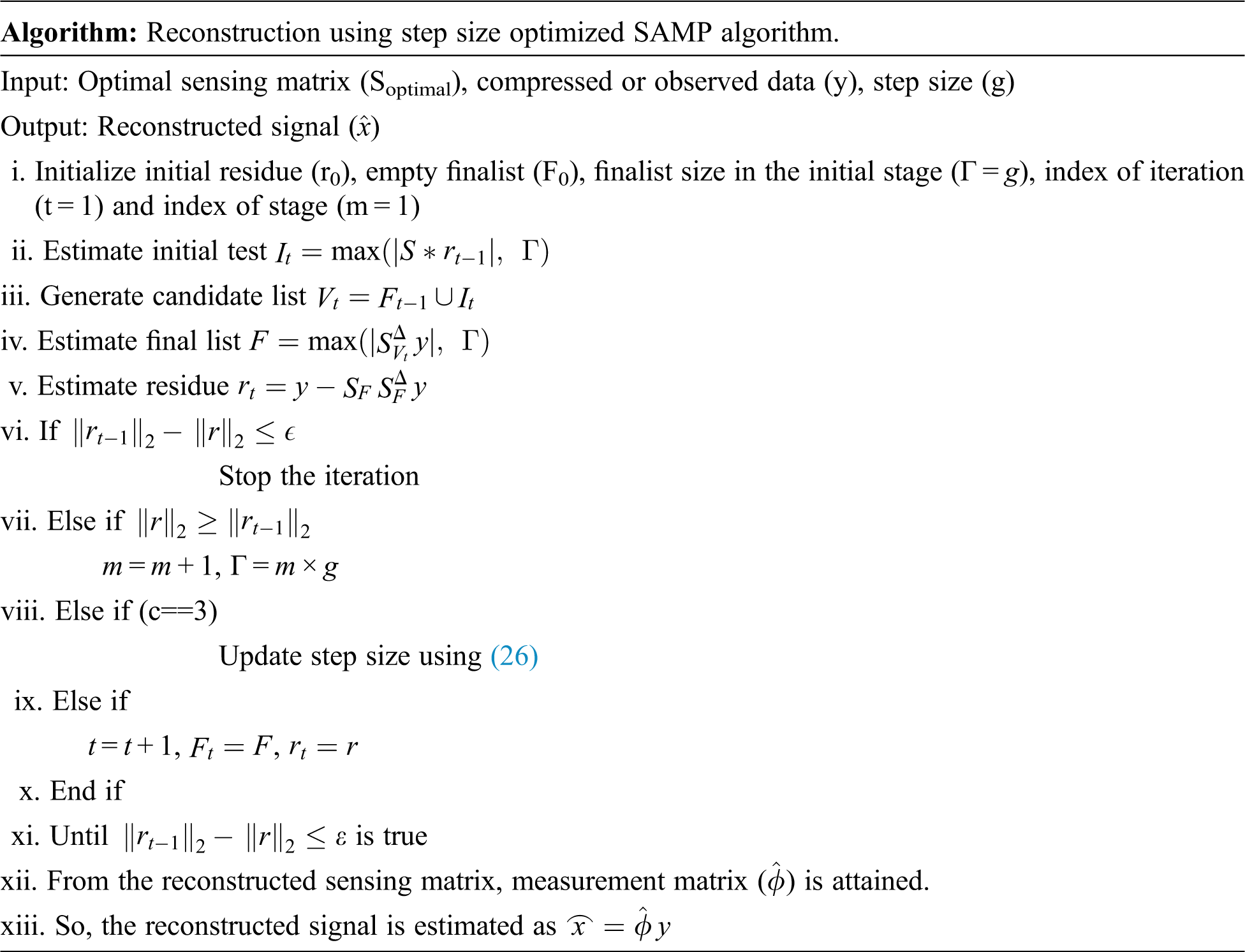
3.4 Reconstruction Using Step Size Optimized SAMP

Data compression is further enhanced by refining the sensor matrix using the ROA method. It leads to enhance the performance of reconstruction too. Nevertheless, we present step size varied SAMP reconstruction algorithm which also enhances the performances of reconstruction further.

In 2008, Thong T. Do, introduced the SAMP algorithm. In this algorithm, sparsity is not considered as priori data for construction. SAMP algorithm is also applicable when the signal has unknown non-zero values. It proposes the staged method i.e., it changes the step to attain the real sparsity of the signal. Additionally, this algorithm incorporates the concept of backtracking into each iteration and workflow of the SAMP algorithm’s in the tth iteration of the stage is depicted in Fig. 2. The workflow of the SAMP algorithm in the tth iteration of s stage is shown in Fig. 2. Unlike OMP and CoSAMP, the SAMP algorithm has adaptive candidate set |Vt| and finalist set |Ft|. Finalist represents the estimated support of signal. Steps of the SAMP algorithm are described as follows.

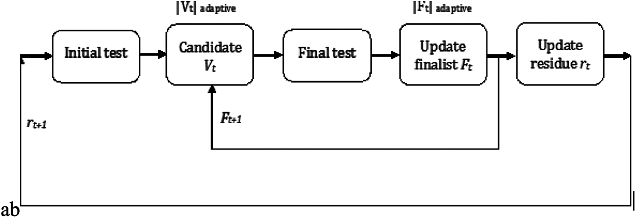
Figure 2: The conceptual diagram of SAMP

Step 1: As shown in the Fig. 2, the initial test and final test are used to generate the finalist. In the block of initial test, the finalist from the set of finalists in the previous stage is selected. As defined in Eq. (17).

It=max(|S∗rt−1|,Γ) (17)

where, It denotes the initial test at iteration t, S denotes the sensing, rt−1 denotes the residue of the previous iteration and Γ denotes the finalist set.

Step 2: Then candidate list is generated by union of the finalist from the previous iteration and short list from the initial test. It is defined using Eq. (18).

Vt=Ft−1∪It (18)

where, Vt denotes the candidate list at tth iteration and Ft−1 denotes the finalist ate previous iteration.

Step 3: The candidate list a subset of coordinates that solves the least square solution is considered the finalist in the block of final test. It is defined mathematically. It is defined using Eq. (19).

F=max(|SVtΔ⁡y|,Γ) (19)

where, SVtΔ denotes the sub matrices of sensing matrix S in candidate list Vt.

Step 4: Finally, due to the subtraction of observation data or compressed samples and the projection of it to the sub matrices in the finalist, the observation residual is updated. Its observation residual is defined using Eq. (20).

rt=y−SF⁡SFΔ⁡y (20)

Step 5: If the algorithm satisfies the halt condition ‖rt−1‖2−‖r‖2≤ϵ , the iteration is stopped. Otherwise, it satisfies the following condition,

If ‖r‖2≥‖rt−1‖2

m=m+1(Update the index of stage) (21)

Γ=m×g(Update the finalist size) (22)

where, m denotes the index of stage, ε denotes the certain threshold and g denotes the first stage.

Else

t=t+1 (23)

Ft=F(Update the finalist) (24)

rt=r(Update the residue) (25)

Step 6: The iteration is updated until halt condition is true.

Step size optimized SAMP: The step size of the SAMP algorithm is increased if the output of an iterative reconstruction does not satisfy the criteria. Additionally, the larger step size in iterations get maintained and this leads to use of ineffective strides in steps. Due to this, the algorithm’s stability and accuracy may be compromised. Thus, to improve the SAMP algorithm’s performance, the step size is improved under particular constrained conditions. So, to enhance the performance of the SAMP algorithm, step size is optimized under certain condition. As shown in the step 5, if ‖rt−1‖2−‖r‖2≥ϵ , the iteration count (c) is updated. If c is larger than 3, the prior step increase is unreasonable at a high probability. Namely, the algorithm does not continue the larger step. At the same time, the count is updated if it is less than 3. The step size optimization is defined in Eq. (26).

g={m×g;m=m−1,if(c==3)gotherwise (26)

The step size is not optimized under the condition ‖rt−1‖2−‖r‖2≤ϵ due to which the iteration gets haulted. Due to this approach, sparsity is recovered accurately in the late step. The algorithm of the step size optimized SAMP is described as follows:

4  Results and Discussions

The proposed scheme is simulated in the platform of MATLAB with the system has the operating system of windows ‘10 with 64 bit and with 4GB main memory at 2 GHz dual-core PC. The MIT-BIH Normal Sinus Rhythm dataset is used in this study. This dataset contains 18 long-term ECG recordings of people referred to Boston’s Beth Israel Hospital’s Arrhythmia Laboratory. The subjects for this dataset were determined to have no significant arrhythmias; they included five men aged 26 to 45 and thirteen women aged 20 to 50. The input ECG signal to the optimized CS framework is shown in Fig. 3a, the compressed ECG signal is shown in Fig. 3b, and the reconstructed ECG signal are shown in Fig. 3c.

Figure 3: (a) Input ECG signal (b) compressed signal (c) reconstructed signal

4.1 The Performance Analysis Based on Sparsity Level

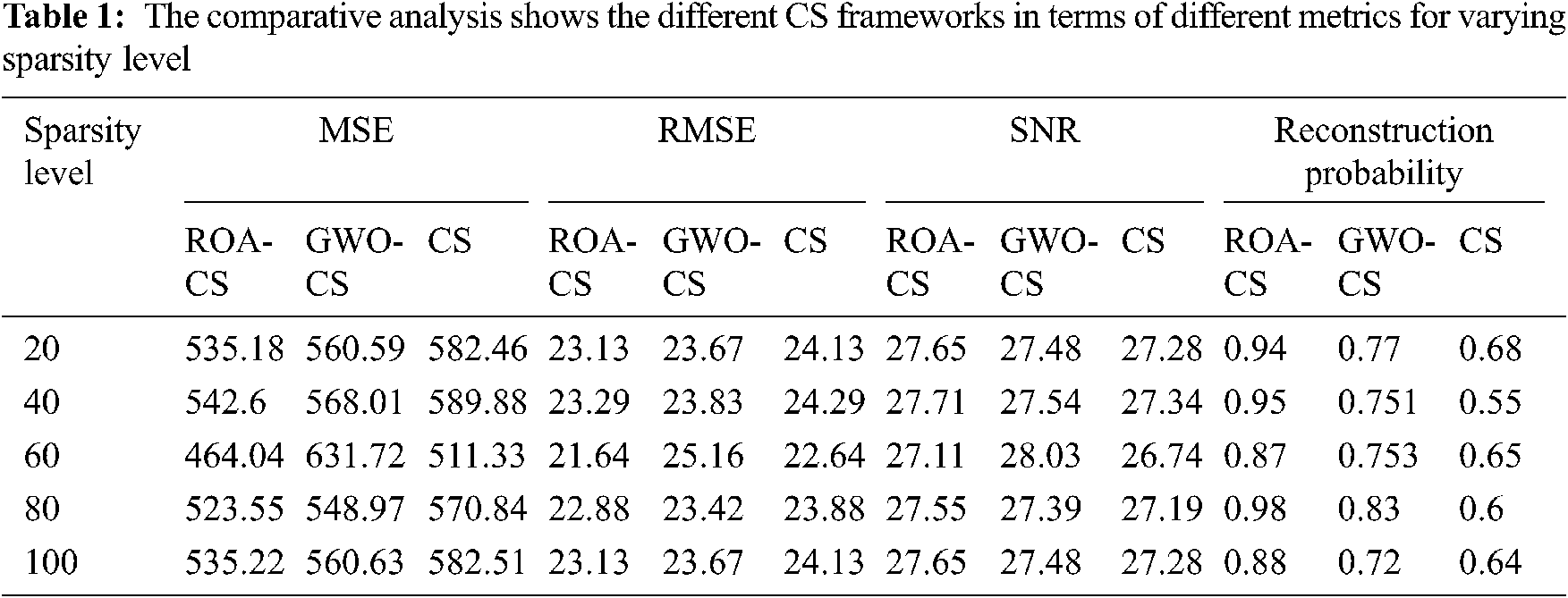
The performance of the optimised CS framework is evaluated in terms of mean square error (MSE), root mean square error (RMSE), signal to noise ratio (SNR), and reconstruction probability for varied levels of sparsity in this section. The comparison analysis in Tab. 1 compares the various CS frameworks in terms of several criteria. As shown in the Tab. 1, the proposed ROA based CS framework is compared with the Gray Wolf Optimization (GWO) based CS [16] and conventional CS. Fig. 4 depicts a comparative comparison of the MSE of various CS frameworks with differing degrees of sparsity where the MSE of the GWO-CS is lower than that of the traditional CS at all sparsity levels except 60 and also due to the optimization of the sensing matrix in the CS using GWO, the CS performed better than the conventional CS. However, compared to GWO, ROA has better convergence speed and adaptability. So, the MSE of the ROA-CS frame work is reduced to 8.3% and 9.2% than that of the GWO-CS and CS respectively.

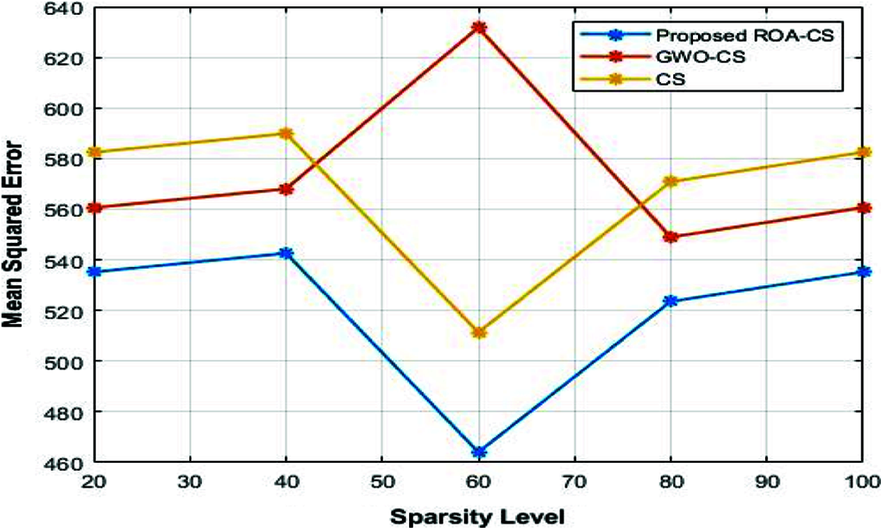
Figure 4: Sparsity level vs. MSE

The comparative analysis of the RMSE of the different CS framework for varying sparsity level is shown in Fig. 5. Compared to GWO-CS and CS, RMSE of the ROA-CS is reduced to 4.2% and 5% than of the GWO-CS and CS respectively. Fig. 6 shows the comparison between different CS frameworks in terms of SNR. Compared to conventional CS, SNR of the GWO-CS is increased except the sparsity level 60. Nevertheless, the optimization of sensing matrix [17] using ROA and the step size optimization of SAMP increase the SNR of CS to 6% and 7.5% than the GWO-CS and CS. The comparative analysis of the different CS frameworks in terms of reconstruction probability for varying sparsity level is shown in Fig. 7. As the reconstruction algorithm SAMP is improved by optimizing [18] step size, reconstruction probability of the ROA-CS increased to 21% and 48% than that of GWO-CS and CS respectively.

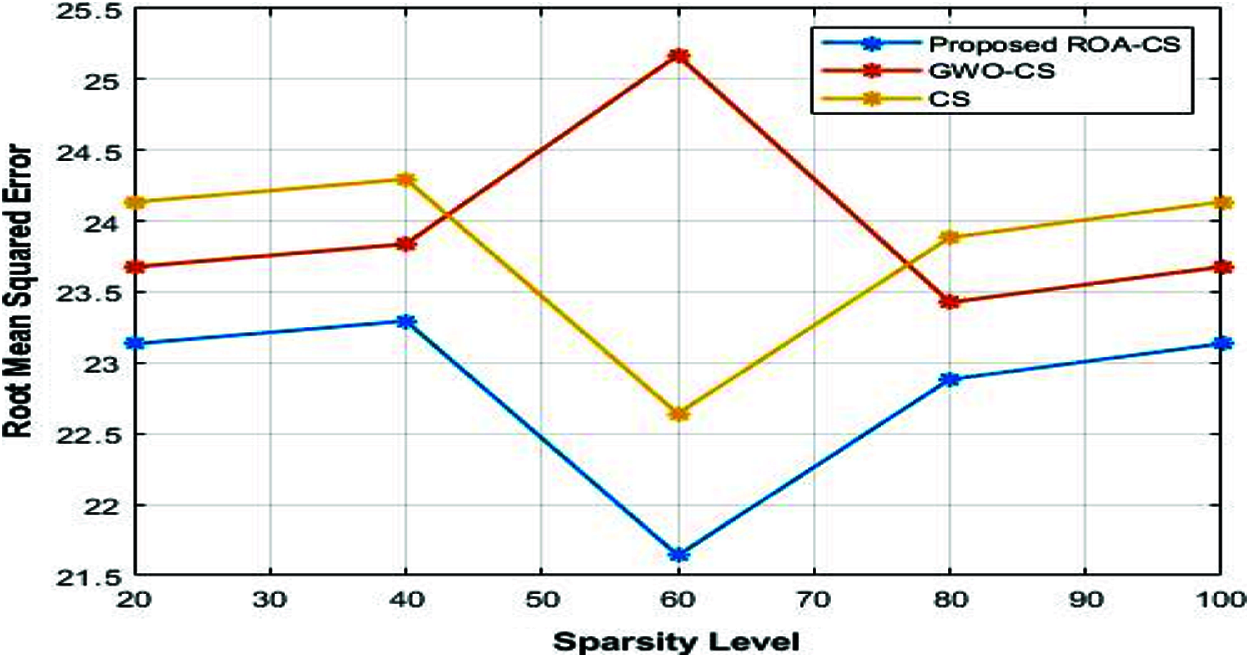
Figure 5: Sparsity level vs. RMSE

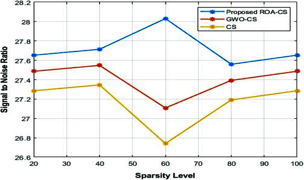
Figure 6: Sparsity level vs. SNR

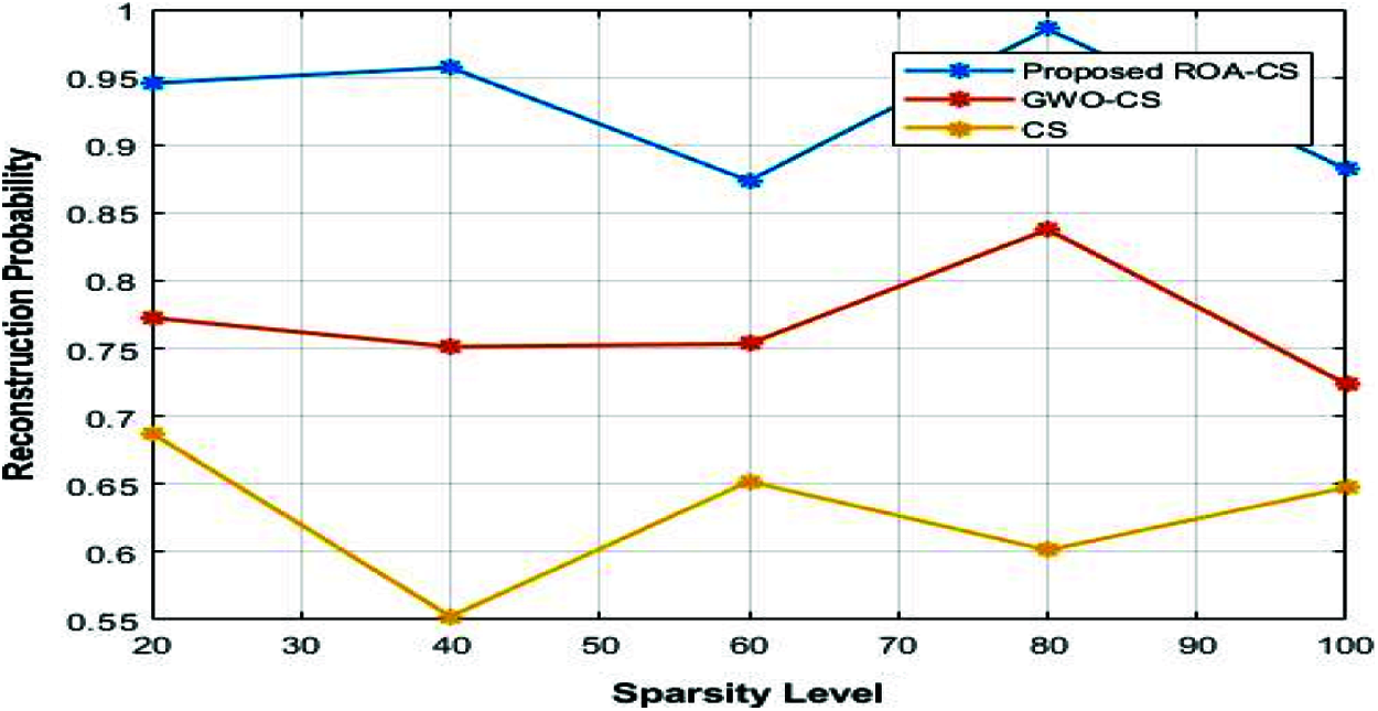
Figure 7: Sparsity level vs. reconstruction probability

5  Conclusion

To enhance the compression rate and reconstruction probability of the CS in WBSN, an optimized CS has been presented in this paper. The performance of the data compression phase been enhanced by optimizing the sensing matrix of CS using rain optimization algorithm (ROA). With the optimal sensing matrix, the reconstruction phase is performed using the step size optimized SAMP algorithm. The performance of the optimized CS framework has been analyzed by varying sparsity level and compression ratio. Besides, the performance of the ROA based CS has been compared with that of the GWO-CS and conventional CS. Additionally, the ROA-based CS performance was compared to that of the GWO-CS and traditional CS. The simulation results indicated that the suggested ROA-CS framework achieved a lower mean square error, root mean square error, signal to noise ratio, and reconstruction probability. In the future, we will focus on enhancing the secure transmission of ECG data in WBSN.

Acknowledgement: The authors with a deep sense of gratitude would thank the supervisor for his guidance and constant support rendered during this research.

Funding Statement: The authors received no specific funding for this study.

Conflicts of Interest: The authors declare that they have no conflicts of interest to report regarding the present study.

This work is licensed under a Creative Commons Attribution 4.0 International License, which permits unrestricted use, distribution, and reproduction in any medium, provided the original work is properly cited.