DOI:10.32604/iasc.2022.021922
| Intelligent Automation & Soft Computing DOI:10.32604/iasc.2022.021922 | |
| Article |
Fault Tolerance Techniques for Multi-Hop Clustering in Wireless Sensor Networks
College of Computer Science and Information Systems, Najran University, Najran, 61441, Saudi Arabia
*Corresponding Author: Adel Rajab. Email: 77adel.rajab@gmail.com
Received: 20 July 2021; Accepted: 20 October 2021
Abstract: Wireless sensor networks (WSN) deploy many nodes over an extended area for traffic surveillance, environmental monitoring, healthcare, tracking wildlife, and military sensing. Nodes of the WSN have a limited amount of energy. Each sensor node collects information from the surrounding area and forwards it onto the cluster head, which then sends it on to the base station (BS). WSNs extend the lifetime of the network through clustering techniques. Choosing nodes with the greatest residual energy as cluster heads is based on the idea that energy consumption is periodically distributed between nodes. The sink node gathers information from its environment that is then transmitted to the base station. The clustering protocol uses a considerably amount of energy for data collection and transmission, with additional energy used for listening to the nodes. It also contributes to channel sensing and avoiding collisions alongside energy transmission. Most clustering techniques do not consider cluster fails, because of which detection through cluster heads or the BS is not possible. Terminated nodes and sub-cluster heads thus continue to transmit information to the failed sub-cluster head, which leads to higher energy consumption. In light of this, we propose a technique to choose cluster heads while reducing the use of CSMA/CA through fault tolerance to determine the failure of the cluster heads by consuming little energy. This work here contributes to increasing the life of the WSN and conserving its energy by more than a half-sensor node per round.
Keywords: Fault-tolerant detection; fault-tolerant recovery; wireless sensor networks; network lifetime; cluster head; energy consumption; fault coverage
Wireless sensor networks (WSNs) are important for the performance of applications in several fields, including military operations, rescue missions, medical surveillance, and climate change. However, a number of issues persist with regard to maintaining connectivity and maximizing the network lifetime in them. The sensor nodes in a WSN directly communicate with one another or with the base station (BS). It is challenging to replace these sensor nodes or recharge them. Therefore, a method is needed to reduce their energy used to extend the life of the sensor network. The optimization of available energy for the sensor node is thus an important operation in the WSN. This end is attained through a clustering algorithm. Clustering is a technique for optimizing the energy consumed during data routing. Clusters are regions of sensor nodes divided into small groups, with each cluster having a node known as a cluster head (CH). Transforming information by using cluster heads reduces energy consumption. In this technique, the cluster heads are close to the BS, to which they can directly transfer their data. Otherwise, they indirectly transfer information to it through multi-hop communication using other clusters. Clustering can thus extend the network’s life. Clustering methods are responsible for collecting data from the environment based on sensor nodes. Other nodes that sense and transfer data only to the cluster heads are known as ordinary nodes [1].
Sensors work together to sense, process, and transfer data. Due to the nature of WSNs, a sensor node, sub-cluster, and cluster head may fail. Therefore, the route from the clusters to the BS may also fail. This study proposes a technique to select cluster heads for the network with a limited use of CSMA/CA through fault tolerance. We propose three basic models: cluster head selection, fault tolerance detection, and recovery. This study modifies LEACH for failure detection and recovery by changing its transformation data to a spare node.
Section 2 presents the protocol specification, and Section 3 summarizes related work in the area. Section 4 examines the protocol implementation, and Section 5 explores its energy efficiency and reliability. Section 6 describes the results of simulation to verify the proposed method, and Section 7 details a comparative examination of it. Finally, Section 8 provides the conclusion of this study and directions for future research in the area.
LEACH [2] employs a distributed algorithm to form clusters. The sensor nodes can make autonomous decisions without any centralized control. The proposed algorithm focuses on the round when a cluster is being formed. Each round begins with a setup phase. Consequently, a steady-state phase formation is used to send data to the sink. The setup phase can be classified into three phases: (1) advertisement, (2) cluster setup, and (3) schedule creation.
As mentioned above, this phase is further classified into three parts.
Each of the nodes yields a haphazard number between zero and one, which is then checked according to a threshold Th(n). If the number is less than Th(n), this means that a cluster head has been selected. Once a sensor node has been selected as the CH, Th(n) is set to zero to allow other nodes a chance of being chosen as the cluster head. Th(n) increases as the number of nodes that are CHs increases. Th(n) self-control increase, thus, the chance for the rest of the sensor nodes to be elected as CHs increases.
T(n) = 1 if only one node is left, meaning that is will certainly be selected. T(n) is given by the equation
where n represents the sensor nodes that can become cluster heads, G represents any node that have not yet been CHs, p represents cluster heads as a percentage of all nodes, and the current round is represented by r. When a node is chosen as the CH, it announces its “id” to the other nodes. Ordinary nodes choose the clusters that they join depending upon the separation between them. Once the cluster heads receive all shared messages, they produce a message to inform every node in their cluster of their status.
Each sensor node decides to join a CH itself. It sends a message to inform the CH that it wants to join its cluster according to the distance between them.
The cluster head accepts the request message from the sensor node to the effect that it wants to be in its cluster. The cluster head knows how many members there are. Thus, it creates a TDMA schedule and permits only a single node to be transferred into each slot. A broadcast of the TDMA schedule is then sent to the cluster members.
2.2 Phase 2: Steady-state Phase
Each sensor node transmits its location information to the cluster head according to its TDMA table time. When all aggregated data have been received by it, the CH resends it to the BS. The latter receives all location information from the CH and retransfers a message to every node to start a new round. This means that the next round cannot begin until the BS has obtain all the data from all CHs in the first round. The algorithm then returns to first stage for CH selection.
In [3], a protocol was proposed for centralized clustering (LEACH-C) in which the base station chooses the cluster head according to the gain in energy and distance from the sink. The BS gathers information on the position and residual energy of every sensor node in the first phase. The base station organizes the residual energy of every sensor. Nodes with low energy are not selected as the CH. The BS is selected as the cluster head, and sends the cluster-id of each CH to every sensor node. The cluster head creates the TDMA for data transfer.
The first round of the E-LEACH protocol randomly selects N nodes as CHs. In the second round, the remaining nodes with high energy are chosen. The protocol improves the LEACH in the setup phase, and is the same as the LEACH protocol in the steady-state phase. The proposed method maximizes the lifetime of the network and balances the load of the network nodes to a better extent than the original LEACH [4].
In protocol selection for TB-LEACH, the CH relies upon a random timer generated by the sensor nodes, and chooses the first advertised node as cluster head from among six or fewer nodes; the other nodes are selected as normal nodes. The lifetime in TB-LEACH is enhanced by over 100 s compared with that in the original LEACH protocol [5,6].
Wang et al. [7] proposed a hybrid multi-hop partition-based clustering routing protocol (HMPBC) that considers cluster head selection with regard to the residual energy of the candidate nodes. Once the large area of the network has been divided into zones, the cluster uses a single-chain structure with only one zone to prolong the lifetime of the network. The minimum spanning tree algorithm through the CHs. The HMPBC solves the problems in multiple LEACH-MLOR [7] and the original LEACH. It uses a minimum spanning tree to communicate with the cluster heads while incurring an additional overhead.
An algorithm to handle network load was proposed in [8] that uses and conserves the residual energy of the idle channel. This is suitable for small WSNs. Another protocol [9], known as improved-LEACH, reduces the energy consumption of every sensor node.
In [10], new techniques were proposed to prolong the network lifetime by reducing the number of messages of the cluster head. The proposed method is called LEACH medium control access (LEACH-MAC). However, it runs into the problems of a large overhead and network complexity. In [11], LEACH simulated annealing was proposed in which the BS is at the center. The method searches for the energy of each node and the distance between sensor nodes according to the center, and the node with the highest remaining energy is nominated as the cluster head.
In [12] a dual-hop-layered LEACH (DL-LEACH) protocol was proposed. It uses two hops between each network node and the BS, and relies on distance. Any node can send data to the cluster head. It first determines the distance between the CH and all BS and then sends the data to the nearest BS.
The authors of [13] proposed a technique called ICH-LEACH that is based on a distance factor that solves the distance problem in LEACH.
The work in [14] improves the PEGASIS to propose a LEACH protocol called EE-RBDG that can enhance energy efficiency, gather information, and reduce the average end-to-end delay compared with LEACH and PEGASIS in each round.
In [15], a protocol was proposed to select cluster heads with a large amount of energy, and is called the EE-LEACH protocol. LEACH-T divides the network into three layers, where each layer has a cluster head [16]. In [17], the authors introduced the LEACH-GA protocol that prolongs the network lifetime compared with LEACH and LEACH-C. O-LEACH, proposed in [18], can improve the throughput and PDR as well as the conserved power energy compared with the original LEACH. In [19], a CH was chosen close to the base station to reduce energy and increase the lifetime of the network.
In [20], a protocol was introduced in which the area of the network is divided into clusters. Each cluster then chooses a cluster head. lGA-LEACH was developed by using a genetic algorithm to select the optimal cluster head and maximize the conservation of power energy by nodes over its lifetime.
The method proposed here considers recent developments (LEACH-MF) to conserve sensor energy. The proposed work focuses on Modified LEACH-MF Parameter and improve its Limited Communication the proposed work called (LC-LEACH-MF). The work enhancement efficiency of Energy Consumption, Packet Delivery Ratio, First Node Dead, Half Node Dead, and Last Node Dead [21].
Syms et al. [22] proposed the suggested ReLEACH protocol that involves choosing a CH for many rounds. This protocol is also known as reappointment LEACH. The node selected as a CH functions continuously until it has lost all energy, at which time another node is chosen as the CH.
Radhika et al. [23] proposed a micro-genetic algorithm-based LEACH protocol (lGALEACH) that uses a genetic algorithm to select the optimal CH. It can improve the network lifetime and reduce energy consumption.
Elmagzoub et al. [24] proposed a thorough, contemporary review of the latest architectures, subsystems and integrated technologies of MIMO wireless signals backhauling using optical fibre access networks.
We propose a technique to select cluster heads for multi-hop clustering in wireless sensor networks. It consists of the following:
• First stage: cluster head selection.
• Second stage: cluster setup.
• Third stage: data transmission.
In the first stage, three sensor nodes with the highest power are chosen. Two of three act as CHs and the third acts as a spare node. In the second stage, the two CHs broadcast an advertisement message to all sensor nodes, which then determine the cluster to join according to the highest and lowest energies. The nodes with the highest energies replay a joint response to the CH to be a multi-hop cluster, and nodes with the lowest energies replay a joint response to the CH or multi-hop node to act as normal nodes. The spare node broadcasts an advertisement message containing information about its id, and stays dormant. The nodes with the greatest energy that function as CHs or multi-hop nodes receive messages regarding the spare node to join according to their failure detection. In the third stage, the two CHs use the TDMA table to collect data from all sensor nodes and transmit them to the BS via the multi-hop connection. The third node uses the TDMA table to gather data from all sensors that detect the failure of sub-cluster heads and transmits this to the BS. The proposed algorithm has the following objectives:
• increase the coverage of WSNs
• fault tolerance
• conserve power by limited use of CSMA/CA
• longer network lifetime
• lower energy consumption
• packets received at the BS
• packets received at the CH
• dead nodes of the network.
The proposed technique focuses on multi-hop communication, which represents the Multi-Hop node fault tolerant technique of sensor node failures in each Multi-Hop clustering in WSNs. The proposed method uses CSMA/CA only in multi-hop clusters and neglects it in normal sensor nodes. This enables the algorithm to conserve the power of all normal nodes. The technique presents fault tolerance as failure detection and recovery. For failure detection, the CHs sends a “hello” message to all multi-hop clusters. If any of these messages is not received, the CH advertises that the given multi-hop nodes is a failed node. The CH sends the failure of transmission of multi-hop information to the spare node to change its valid nodes to the spare node, which transmits the collected data to the base station.
4.1 First Stage: Cluster Head Selection
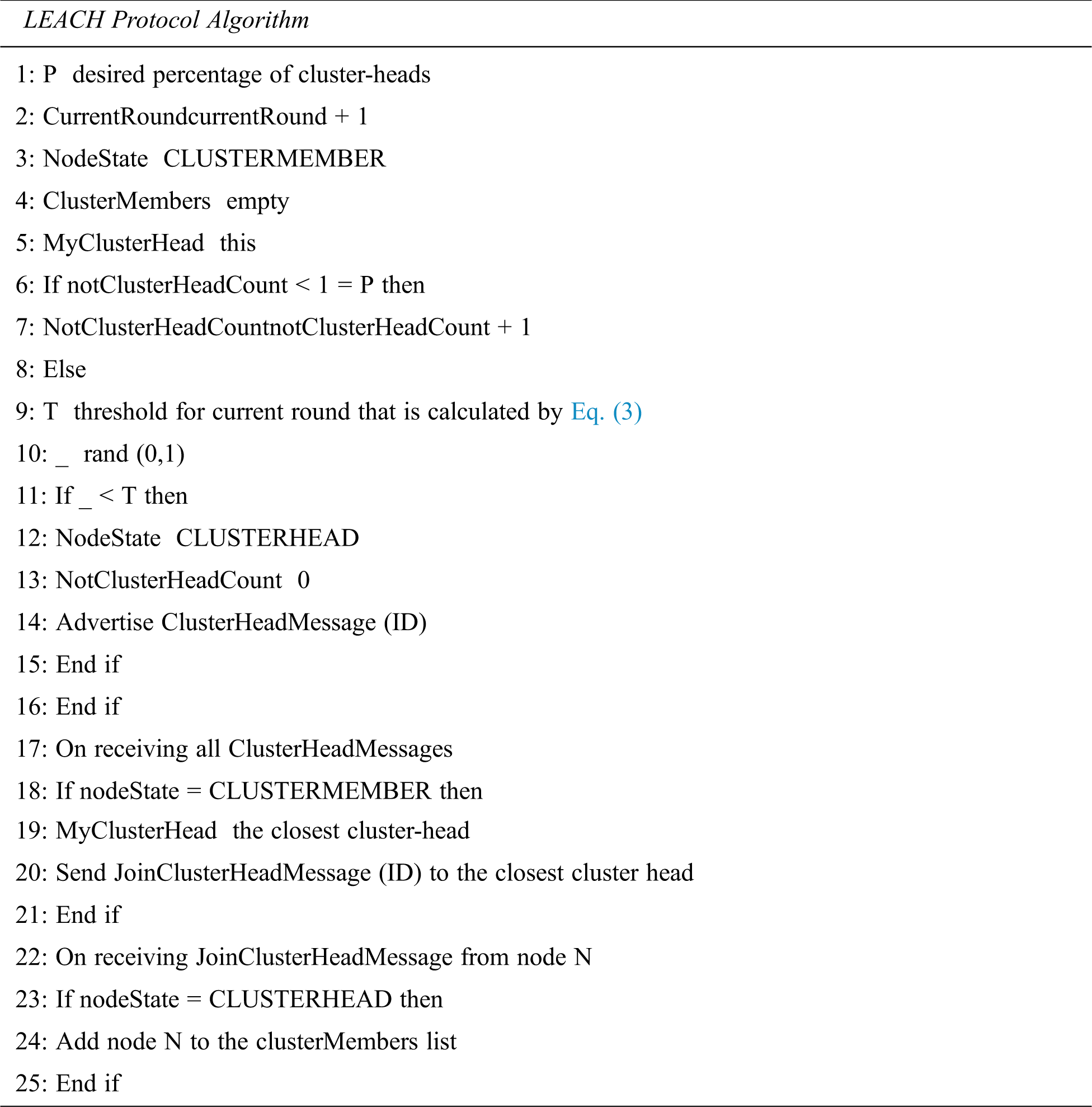
The proposed technique selects the nodes with the greatest energy as the CH. Two nodes are identified as CHs, and a tree is built around them as shown in Fig. 1, where Counter Left = 0 and Counter Right = 1.
The first point on the tree is built by using N-Counter Left (representing the first point on the left branch) and Counter Right + 2 (representing the first point on the right branch). Counter Left and Counter Right are increased by one, and move to the second point. The left branch is built here by using N-Counter Left (representing the second point on the left branch) and Counter Right + 2 (representing the second point on the right branch). The third point (a spare node) is used only if multi-hop failure is identified by the failure algorithm. If more than 10 sensor nodes are used, Counter Left and Counter Right are both increased by one and all the above steps are repeated. This generates many branches of the tree with higher energies on the right side than the left. The nodes of the right branch become multi-hop nodes for other nodes. The tree is rebuilt by resetting Counter Left and Counter Right to zero and one, respectively, at beginning of each round.
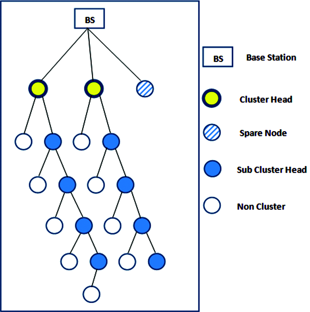
Figure 1: The clustered architecture with 20 nodes
4.2 Second Stage: Cluster Setup
The proposed method chooses three nodes with the highest energy. Two of them act as cluster heads and the third one is a spare node. The CHs then broadcast advertisement messages containing information about them and their ids. The spare node broadcasts an advertisement message containing information on its id. Based on their remaining energy, the sensor nodes identify the CH to join. The multi-hop cluster and the normal nodes then replay a response message to the CH.
4.3 Third Stage: Data Transmission
The CHs use the TDMA table to gather data from all network nodes that are then transmitted to the BS, as in the original LEACH protocol. Each sensor node selected as the CH is responsible for collecting data from the other sensors. Both the CHs then create a TDMA table of active members. As in the original LEACH method, the two CHs or the spare node collect data from surrounding nodes that are then sent to the BS. This process is shown in Figs. 2–4. The algorithm rebuilds the TDMA in each round.
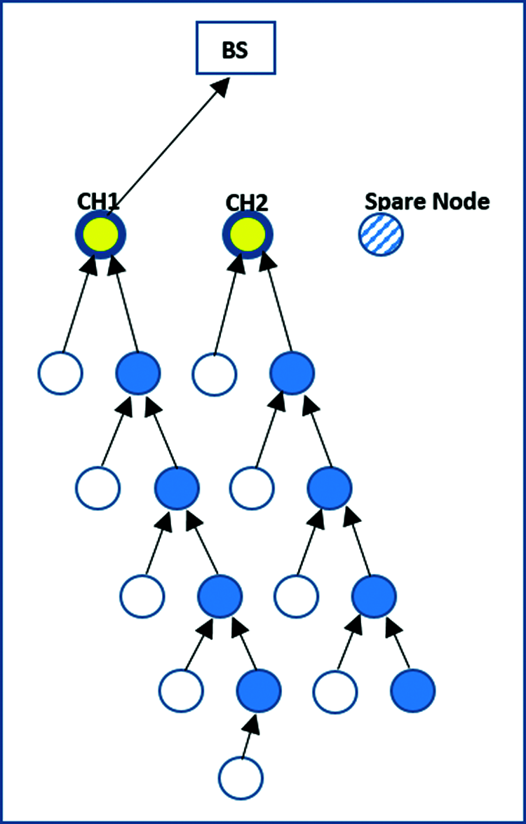
Figure 2: Data transmission by the first cluster head
Fig. 2 shows that the first cluster (CH1) collects all information from its members. This is followed by CH2 and the spare node. CH1 collects information received from the normal sensor nodes and its multiple hops, and transfers it to the BS. The work here is distributed among the main three sensor nodes. This provides a benefit from the corruption of low power to transfer its message before dissipating its energy. It also helps conserve power and prolong the network’s lifespan.
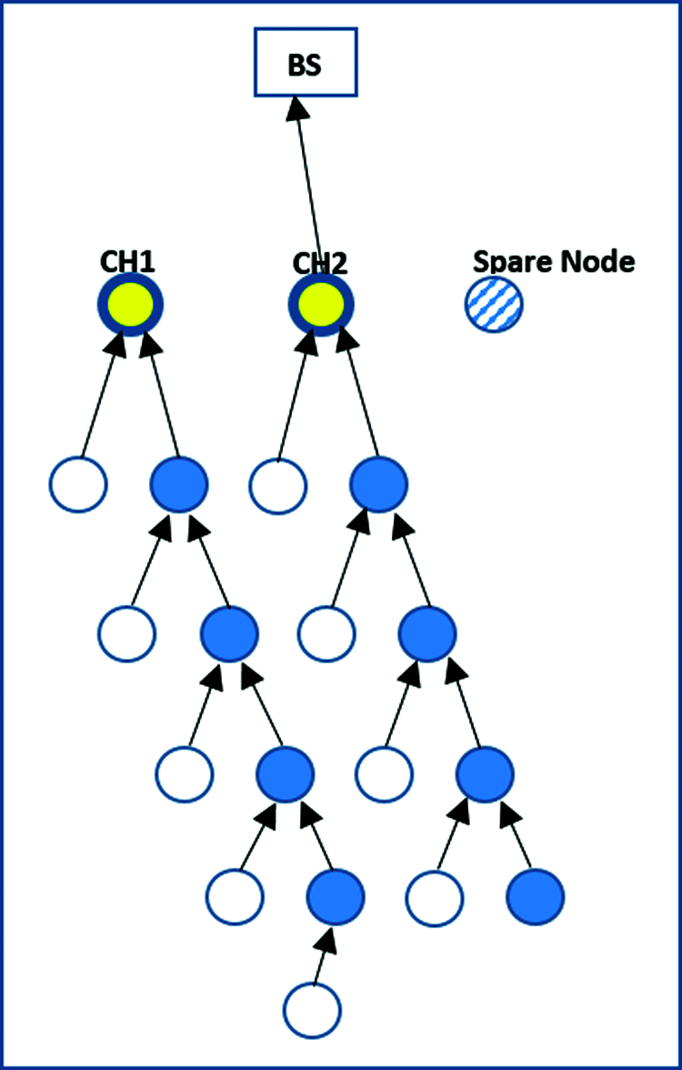
Figure 3: Data transmission by the second cluster head
Fig. 3 shows that the second cluster head (CH2) collects information from normal sensor nodes reachable through multiple hops in its cluster area, followed by the spare node, and resends it to the BS.
Fig. 4 shows a spare node working as the third cluster head, which is only found if that the multi-hop cluster failed, whereby it will receive the information from its members and compare it with first and second clusters. The spare node gathers the data from its normal sensors and multi-hop nodes according to its cluster area, and resends it to the BS.
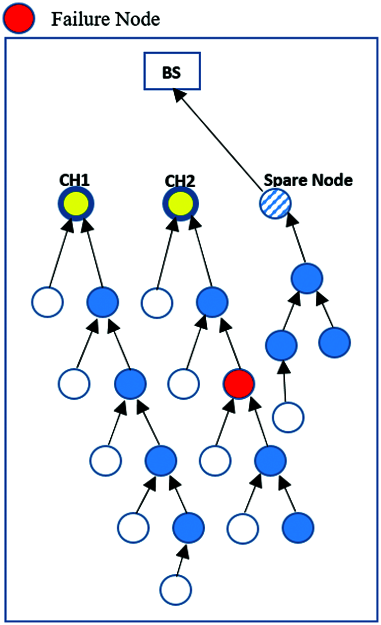
Figure 4: Data transmission from spare node
5 Energy Efficiency and Reliability
The proposed objective is to conserve the energy of the sensor nodes by limiting the use of CSMA/CA, which consumes a significant amount of power in the transmission and receipt of data to sense the channel.
We explain the probability of data transmission to conserve energy. k represents the number of packets to transmit to the TDMA slot from the cluster head. Our method distributes the packets over the nodes by considering the worst possible collisions. CSMA transmits a packet if the channel is clean, and all other sensor nodes in it abort their attempts and sense its transmission. The channel can be by c parameter and p persistent the CSMA-slot. The proposed [3] assumes that all packet transmissions are lost if more than one sensor node accesses the channel slot. In these works, the probability of the first CSMA-slot which receives successful transmission is in equation:
The next CSMA slot receives its successful transmission, given by:
The cluster forwards k−1 packets by using the CSMA slot with the highest probability of successful transmission.
Cluster behavior is represented as a discrete-time Markov chain (DTMC), as shown in Fig. 5. It shows the number of sensors states that a packet must forward. State 0 is the steady-state solution of the chain. The CSMA has the following probability of containing at least one sensor node that attempts to transmit a packet:
CSMA focuses on two bounds: failure occurring in case of two simultaneous sensing procedures, and when a sensor node initiates a transfer between the posting and the execution of the sending task of another node. To solve the problem of incorrect sensing if two sensors are involved, the following equation is used:
where $ represents the probability of incorrect sensing between the sensors, and $ parameter is closer to the 1, p (K−1) refers to the expected number of additional accesses to the channel in the same CSMA slot.
5.1 Fault Tolerance as Failure Detection
To detect the failure of a CH, we modify our proposed algorithm. Let the time of beginning of a round be represented by btr. btr + fn represents the time at which the second round begins, and fn presents the duration of one round. We chose three main sensor nodes, of which the two with the highest energy were used as cluster heads and the third as the spare node. A total of m sensor nodes represented a part of the multiple hops transmitting the data for s seconds to the cluster’s TDMA table. For each cluster transfer, t1 = fn* m/s represents transmission through the CHs and their sensor nodes. The cluster heads transfer a message to only other cluster heads and multi-hop nodes. The CHs heads use time t1 to detect a transmission that has not been received by the multi-hop nodes. The proposed method neglects ordinary sensor nodes in the detection in each round, and identifies only multi-hop nodes if a transmissions has failed. The CHs can advertise the failure of the multi-hop node as shown in Fig. 5.
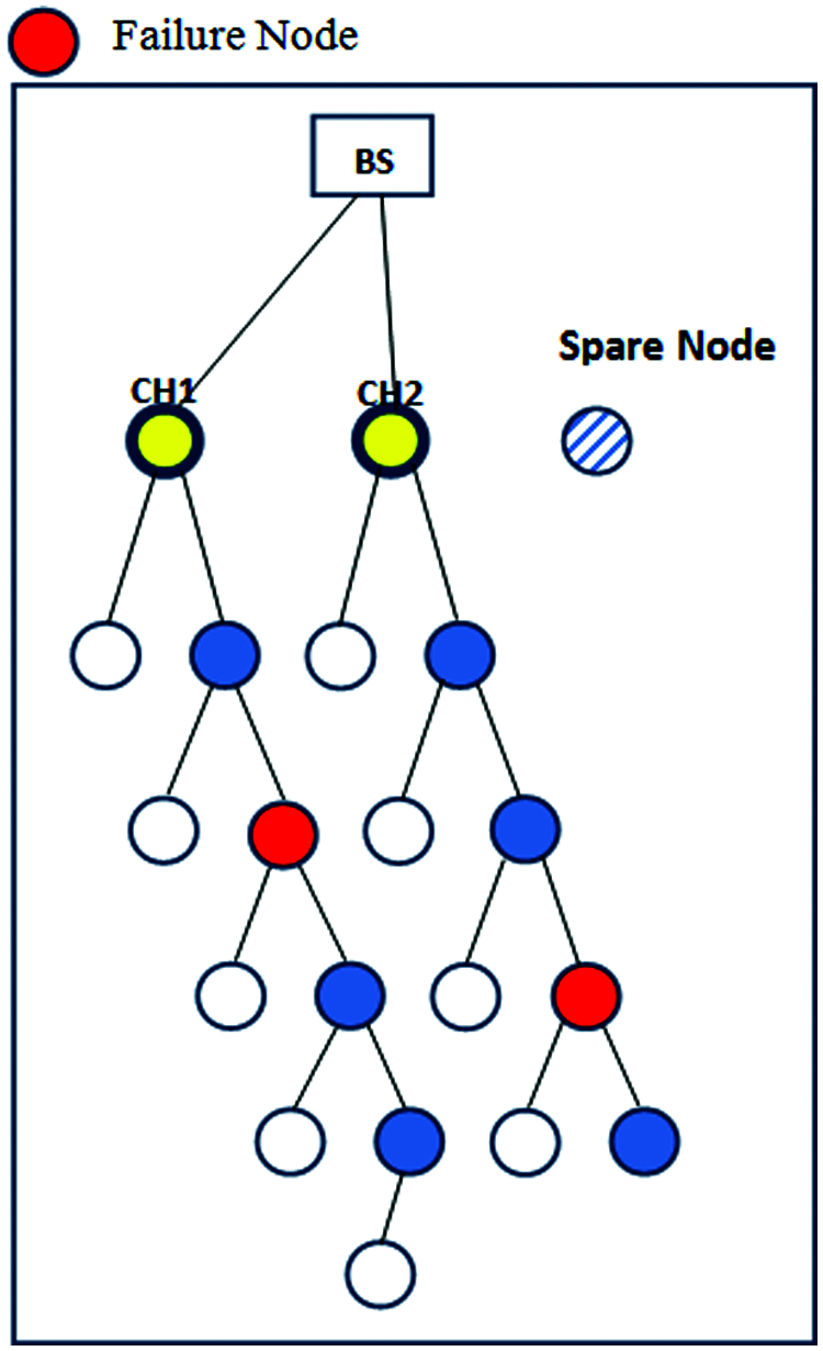
Figure 5: Failure detection
5.2 Fault Tolerance as Failure Recovery
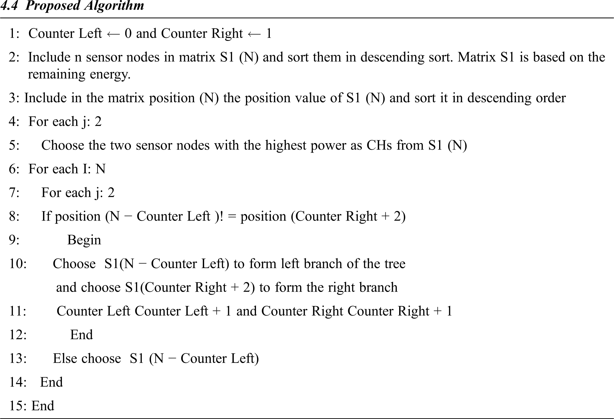
If the failure of a multi-hop node is detected, the fault tolerance recovery model informs the multi-hop failure + 2 node to become the new multi-hop according to its positional value. And join a position of multi-hop failure + 2 to a spare node. Also, the normal nodes which join before to a multi-hop node failed, it joins by using the n-(multi-hop failure + 2) − 1 to a spare node, according to its position value, as shown in Fig. 6.
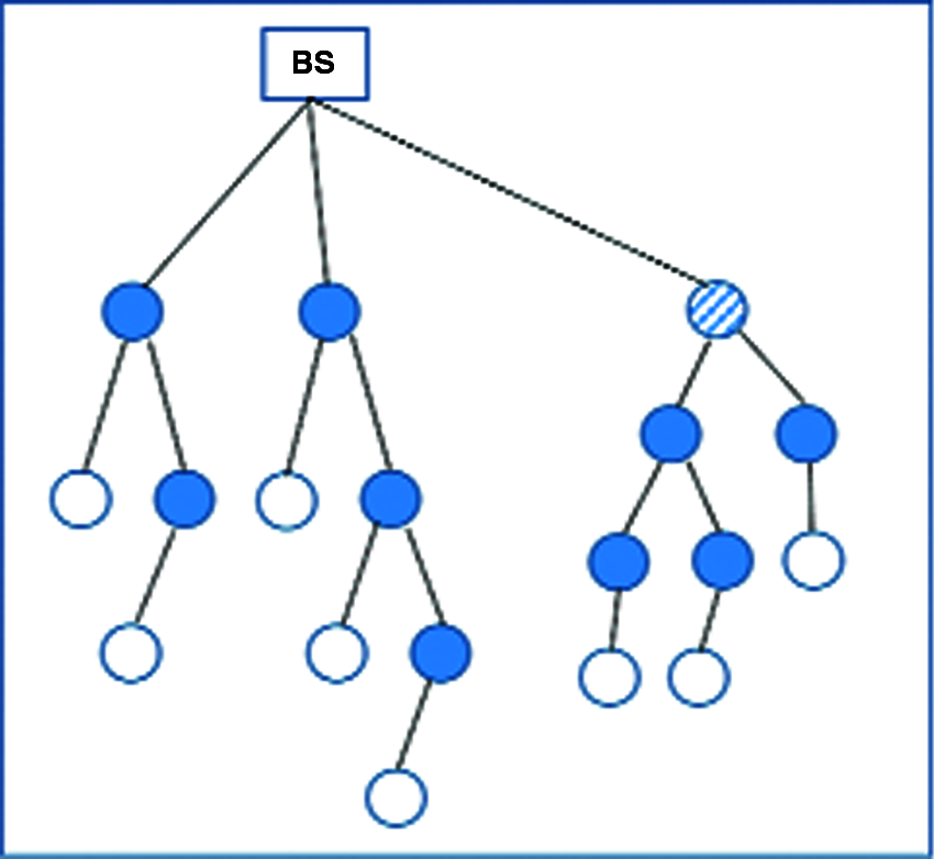
Figure 6: Cluster head recovery in WSN
Each CH has members, a multi-hop node and normal sensor nodes. The first and second clusters with them multi-hop nodes only in each cluster represent a chine. So, the total of chines in this techniques are two, such as in Fig. 7.
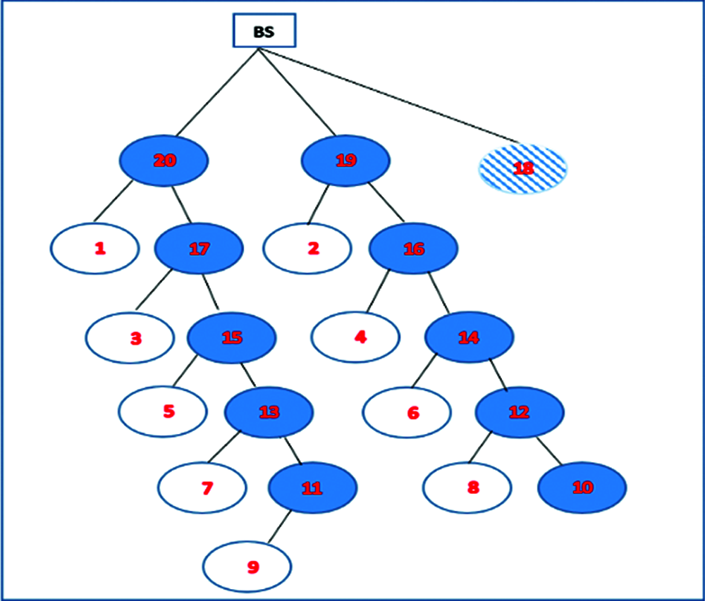
Figure 7: The chine architecture of a cluster head
Nodes 20, 17, 15, 13, and 11 in the above represent the first chain, and nodes 19, 16, 14, 12, and 10 represent the second chain. Node 10 is terminal in the second chain. These nodes hereinafter neglect failure, but can become clusters or sub-clusters after a set of rounds; during this time, the algorithm starts examining its nodes to identify failure. We neglect two sensor nodes per each two-chain sequence, which causes these nodes to change into normal sensor nodes that constitute more than half of all nodes in the network. This helps retain more energy in each round. Fault-tolerant coverage is an important issue in any technique for detecting and recovering from the failure of nodes in a sensor networks.
The probability of failure nodes occurring in a single chain is as follows:
where F_Node is the probability of faulty nodes occurring among N_S_Chain nodes.
N_S_Chain represents the number of nodes in a single chain.
The probability of failure of the first chain of sensor nodes is calculated by the following equation:
The probability of failure of the second chain of sensor nodes is as follows:
F_Node represents the probability of a node being faulty among N_S_Chain nodes.
F_Node1 represents faulty nodes in chain1, F_Node2 represents faulty nodes in chain2, N_S_Chain1 represents the number of sensor nodes in chain1, and N_S_Chain2 represents number of sensor nodes in chain2.
For example, if N_S_Chain1 = 4 the number of sensor nodes of chain1 and F_Node1 = 2 failure sensor nodes among a N_S_Chain1, it calculating as:
The total number of faulty sensor nodes in the first and second chains is calculated as follows:
The exhaustion of power for detect a sensor nodes failure bases on the CHs and multi-hop nodes. The CHs transfer messages to the multi-hop nodes and neglect the normal member nodes. Therefore, they use more power more than normal sensor nodes, which constitute most nodes of the sensor network. These techniques can conserve more power in each round. The proposed, CHs transfer acknowledgment of a fault multi-hop nodes excepted the normal sensor nodes which are ready to becoming as a multi-hop nodes in a coming round, when the multi-hop nodes accept a messages coming from the CH, and resend acknowledgment message to its CH. The normal nodes are prevented from receiving or sending any acknowledgment. Therefore, energy is conserved until these nodes becomes CHs or multi-hop nodes. Thus, the faulty messages required are: 2* (2* (N_S_Chain − 2)).
The total power consumed for failure detection is:
where ETx (k, d) and ERx (k)) are as follows:
There are two chains, and two messages are required.
Power of recovery of failure nodes is given by:
The fault-tolerant power is given by:
Simulations were implemented in a square area of l00 m × l00 m with an initial energy of 2 J to deploy 100 sensor nodes. The simulation was executed in MATLAB. We implemented the original LEACH algorithm, LC-LEACH-MF, and our proposed method that contains fault tolerance techniques. We simulated a number of rounds to measure the lifetime and power consumption of the nodes to detect and recover the failed nodes. The proposed method consumed less power compared with the original LEACH algorithm and LC-LEACH-MF. It increased the coverage and lifetime of the WSN as shown in Tab. 1 and Fig. 8. We assessed our method in terms of the number of live nodes, number of dead nodes, energy consumed for identifying a fault (detection, recovery), and energy consumed by the live nodes.
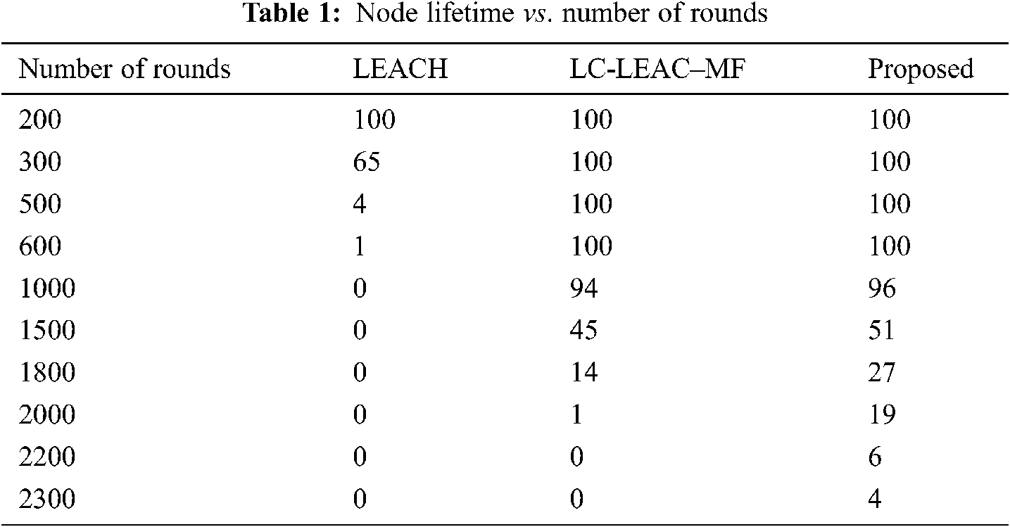
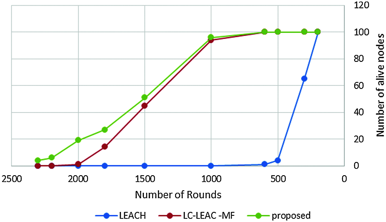
Figure 8: Lifetime measured in rounds
Network lifetime or the number of live nodes is the total lifetime of the network from the start of the round until the last dead node. Tab. 2 and Fig. 9 shows a comparison among the original LEACH, LC-LEACH-MF, and our proposed protocol in terms of network lifetime. Nodes of the LEACH protocol began to die starting from round 300, the first six nodes of the LC-LEACH-MF protocol died in round 1,000, as did four nodes of our proposed protocol. The proposed network nodes die at around 2274, but in our proposal that is up to around 2300. Therefore, the proposed method was superior to the LEACH and LC-LEACH-MF protocols.
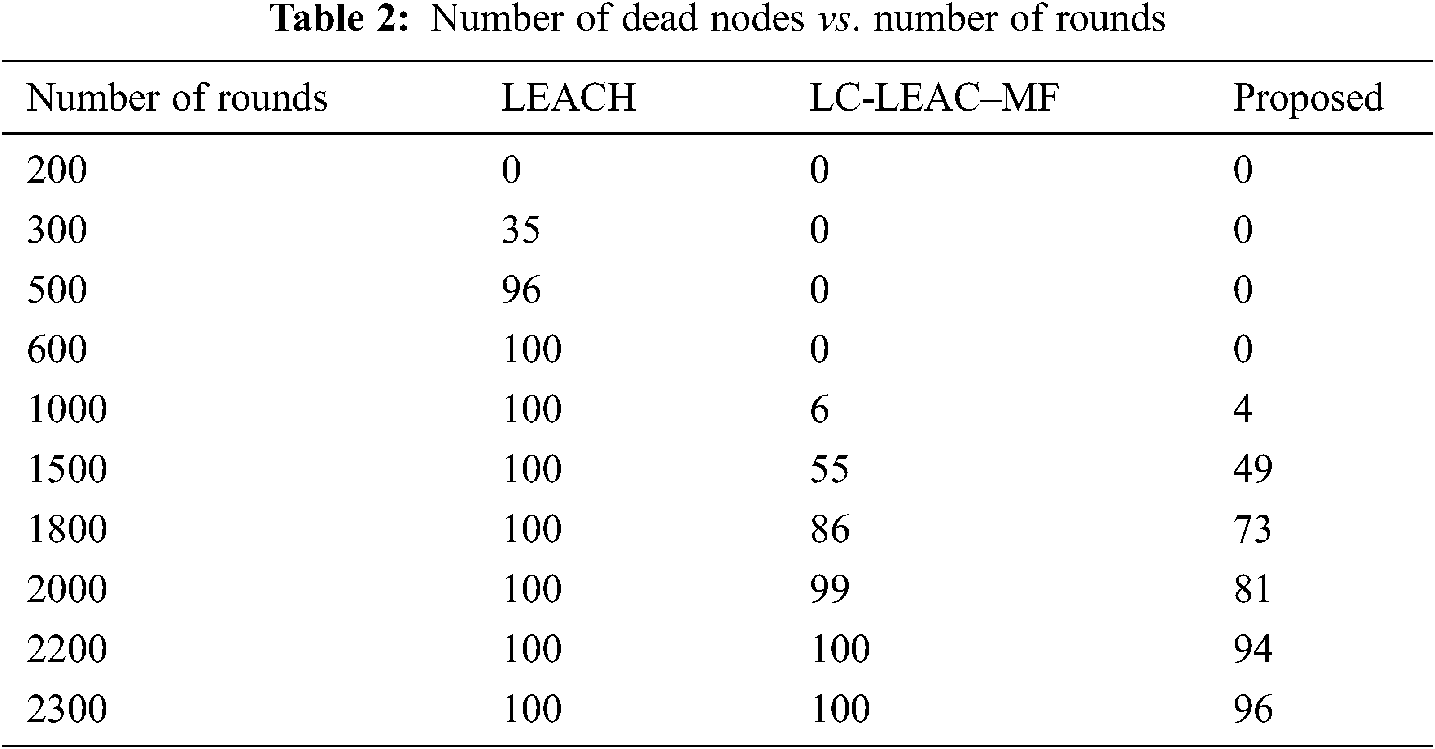
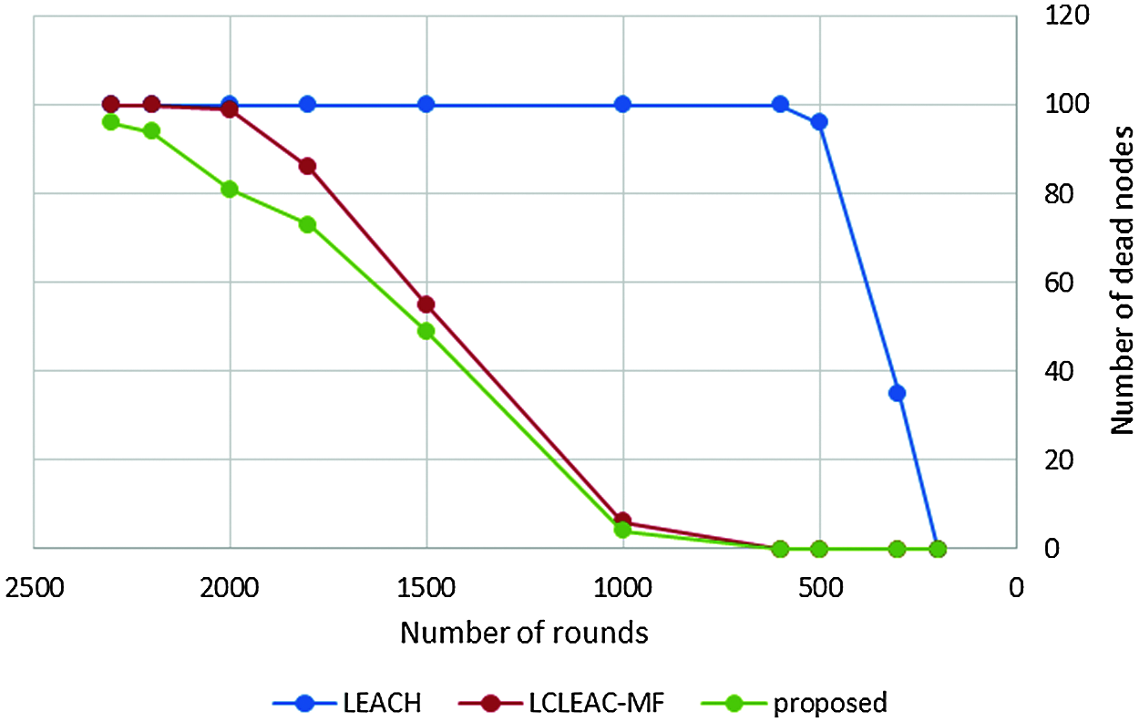
Figure 9: Analysis of number of dead nodes vs. number of rounds
Tab. 3 and Fig. 10 show a comparison among the LEACH, LC-LEACH-MF, and our proposed method in terms of first node dead (FND). It shows that the proposed method suffered from an earlier FND than the LEACH and LC-LEACH-MF protocols.
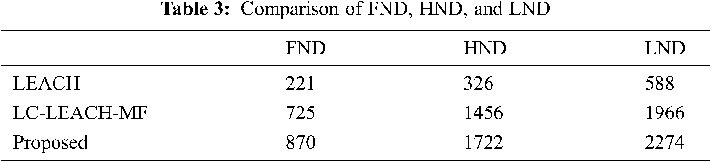
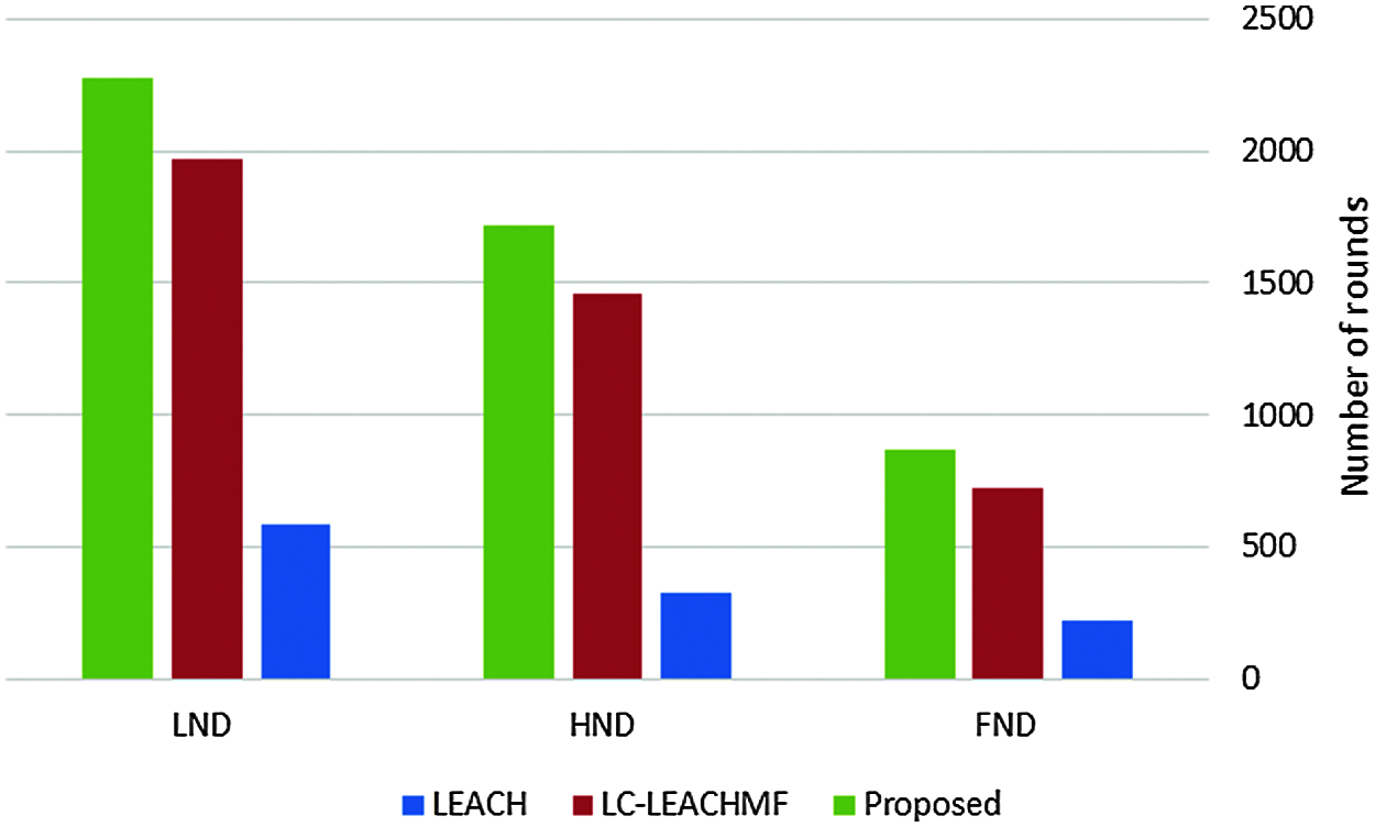
Figure 10: Analysis of FND, HND, and LND vs. number of rounds
Tab. 4 and Fig. 11 show that the proposed method was more efficient than the LC-LEACH-MF and the original LEACH protocols in terms of energy consumption. At close to round 300, the LEACH protocol had expended all its energy, while at around 600 the LC-LEACH-MF consumed its energy, and at around 2200. Our proposed protocol therefore gains the highest energy, consumed at around 2300. Thus, the proposed work is improved in the comparison of LEACH and LC-LEACH-MF protocols in terms of energy consumption. Tabs. 5 and 6, and Figs. 12 and 13 show the lowest amount of energy for the detection of a failure node.
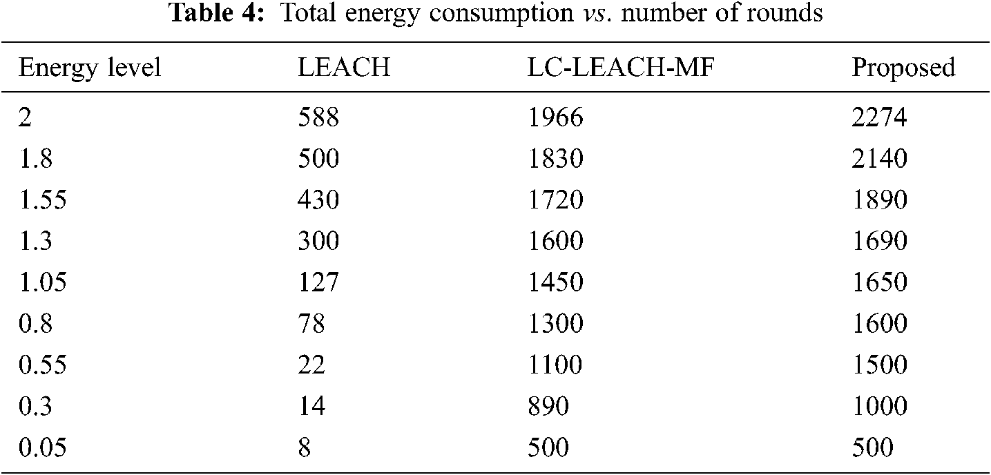
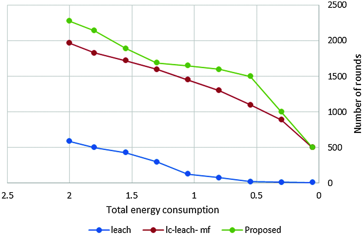
Figure 11: Total energy consumption vs. number of rounds
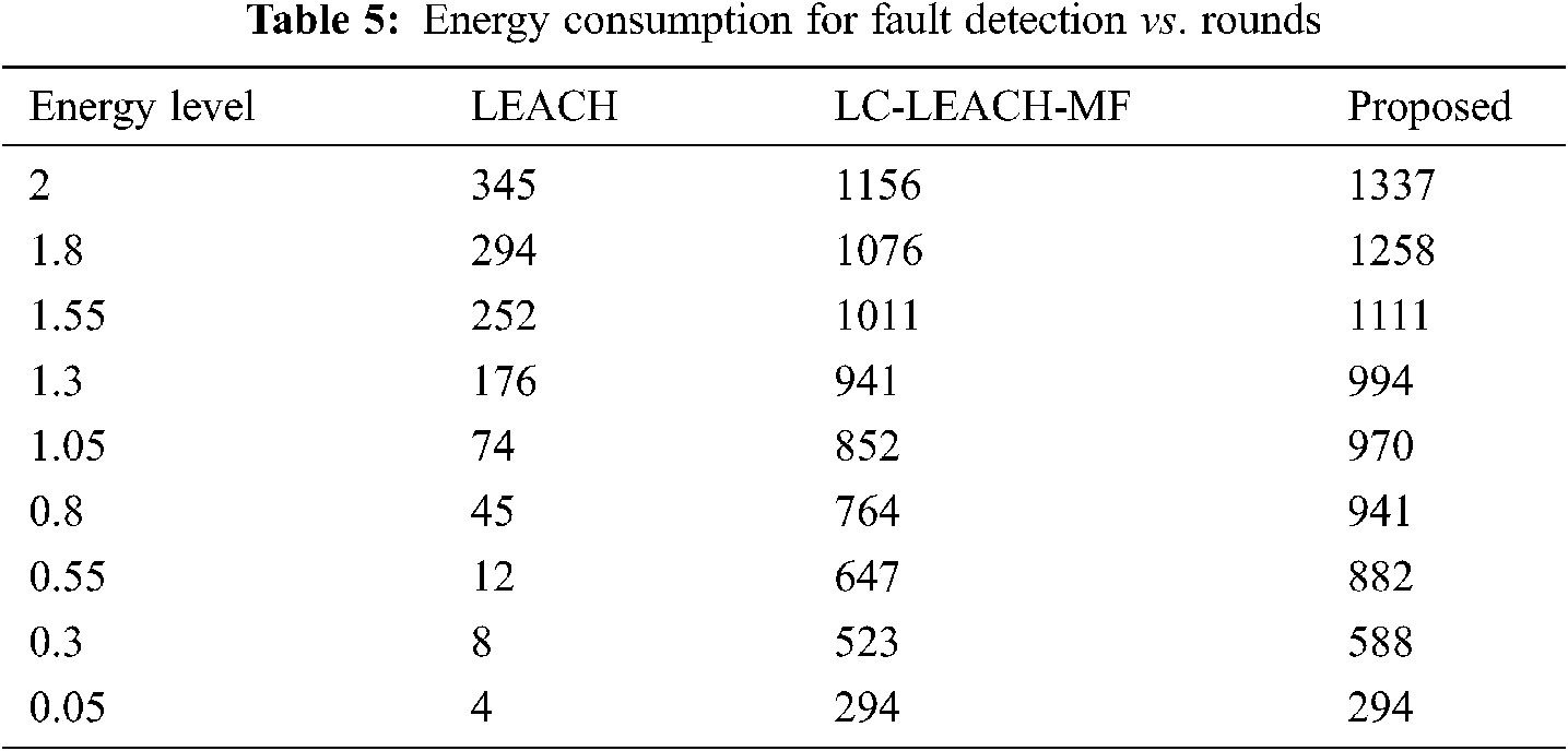
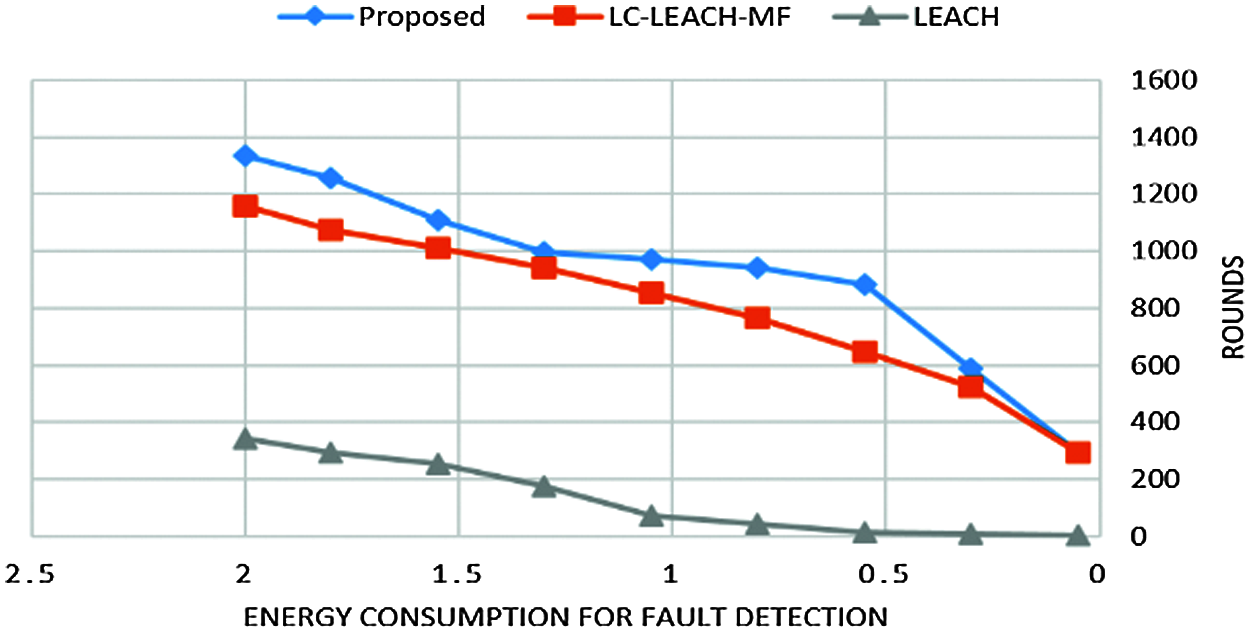
Figure 12: Energy consumption for fault detection vs. number of rounds
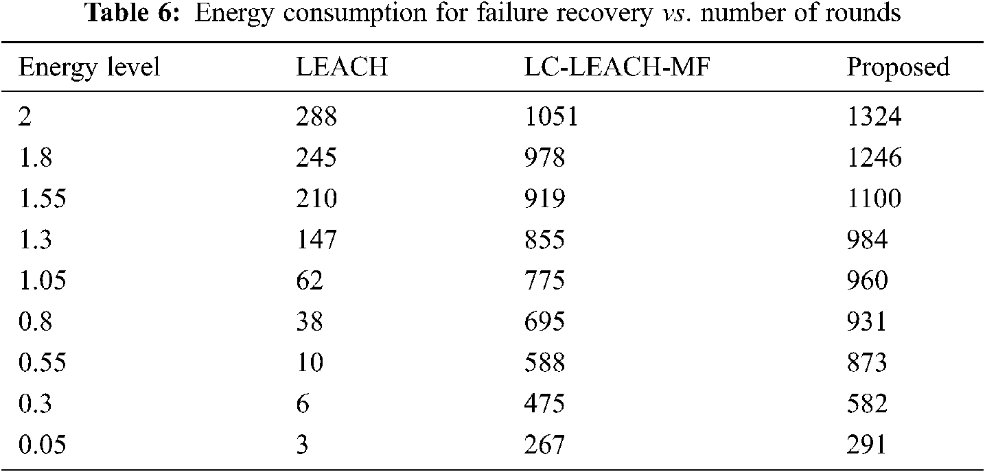
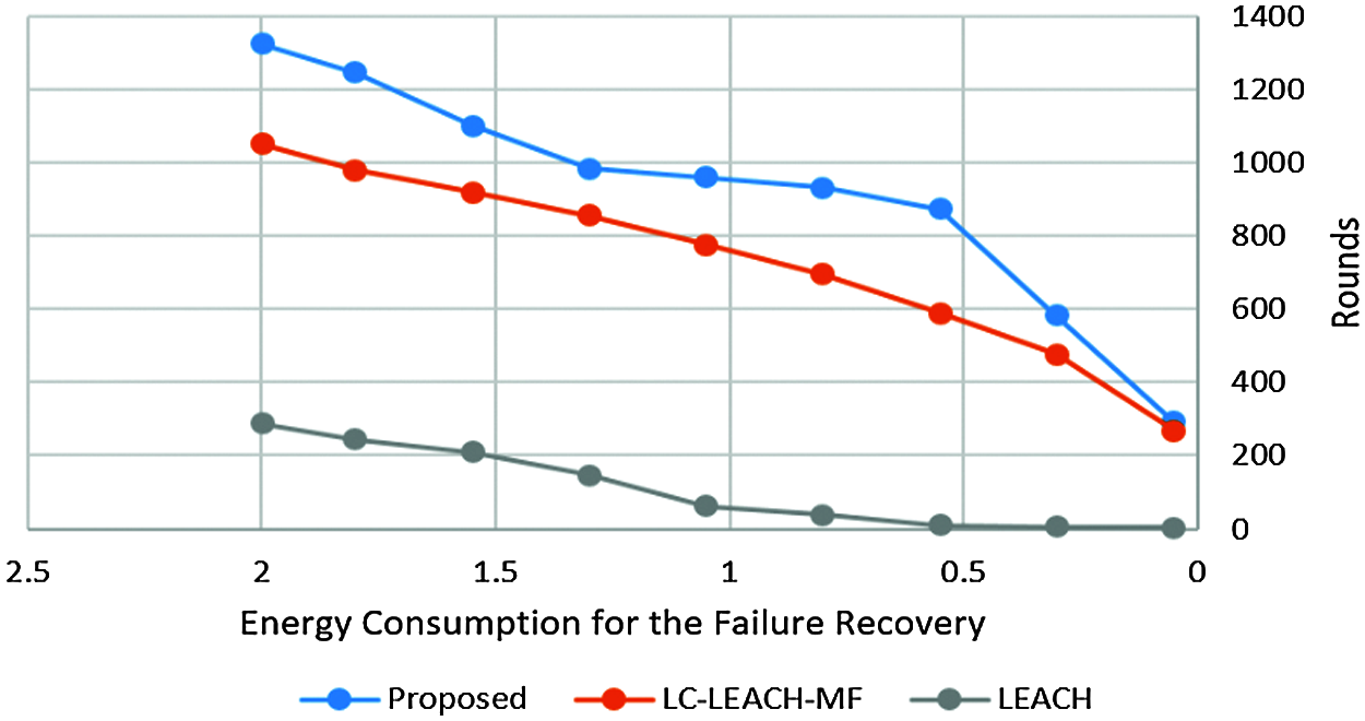
Figure 13: Energy consumption for failure recovery vs. number of rounds
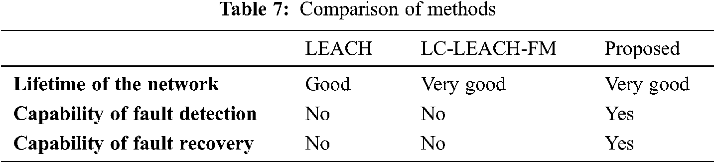
We compared LEACH, LC-LEACH-FM, and the proposed method in terms of network lifetime, fault detection, and fault recovery, where the comparison reveals the three protocols which improved the network lifetime, which is the best one of three protocols. LEACH and LC-LEACH-FM do not contain fault tolerance techniques while the proposed method does, as shown in Tab. 7.
In this study, we proposed a method to reduce the energy consumed by a WSN by using a limited amount of CSMA/CA compared with the LEACH protocol, by detecting and recovering the failure of cluster heads or sub-cluster heads. The proposed techniques can conserve over half of sensor energy in each round. It exhibits better fault tolerance than LEACH and LC-LEACH-FM [21]. In future work, the performance of the proposed protocol should be investigated by taking into account the ratio of packets delivered to the cluster heads and the base station, the end-to-end delay, overhead, and distance.
Funding Statement: The author received no specific funding for this study.
Conflicts of Interest: The author declare that he has no conflicts of interest to report regarding the present study.
1. S. Mahajan and P. K. Dhiman, “Clustering in wireless sensor networks: A review,” International Journal of Advanced Research in Computer Science, vol. 7, no. 3, pp. 198–201, 2016. [Google Scholar]
2. W. B. Heinzelman, “Application-specific protocol architectures for wireless networks,” Ph.D. Dissertation, Department of Electrical Engineering and Computer Science, MIT, Cambridge, MA, (Accessed 8 October 20202020. [Online]. Available: https://dspace.mit.edu/handle/1721.1/26881. [Google Scholar]
3. W. B. Heinzelman, A. P. Chandrakasan and H. Balakrishnan, “An application-specific protocol architecture for wireless microsensor networks,” IEEE Transactions on Wireless Communications, vol. 1, no. 4, pp. 660–670, 2002. [Google Scholar]
4. M. Mumtaz, A. Mumtaz and M. N. Khan, “Energy aware routing using improved LEACH protocol,” Universal Journal of Communications and Network, vol. 3, no. 3, pp. 64–67, 2015. [Google Scholar]
5. J. Hu, Y. Jin and L. Dou, “A time-based cluster-head selection algorithm for LEACH,” in IEEE Symp. on Computers and Communications, Marrakech, Morocco, pp. 1172–1176, 2008. [Google Scholar]
6. R. P. Mahapatra and R. K. Yadav, “Descendant of LEACH based routing protocols in wireless sensor networks,” Procedia Computer Science (Elsevier), vol. 57, no. 1, pp. 1005–1014, 2015. [Google Scholar]
7. C. Wang, Y. Zhang, X. Wang and Z. Zhang, “Hybrid multihop partition-based clustering routing protocol for WSNs,” IEEE Sensors Letters, vol. 2, no. 2, pp. 1–4, 2018. [Google Scholar]
8. Z. Peng and X. Li, “The improvement and simulation of LEACH protocol for WSNs,” in IEEE Int. Conf. on Software Engineering and Service (ICSESSBeijing, China, pp. 500–503, 2010. [Google Scholar]
9. A. Latiwesh and D. Qiu, “Energy efficient spectrum aware clustering for cognitive sensor networks: Cog LEACH-C,” in 10th Int. Conf. on Communications and Networking, China (ChinaComShanghai, China, pp. 515–520, 2015. [Google Scholar]
10. C. Tang, Q. Tan, Y. Han, W. An and H. Li, “An energy harvesting aware routing algorithm for hierarchical clustering wireless sensor networks,” KSII Transactions on Internet and Information Systems (TIIS), vol. 2, no. 2, pp. 504–521, 2016. [Google Scholar]
11. H. Zhang, H. S. Zhang and W. Bu, “A clustering routing protocol for the energy balance of wireless sensor network based on simulated annealing and genetic algorithm,” International Journal of Hybrid Information Technology, vol. 7, no. 2, pp. 71–82, 2014. [Google Scholar]
12. J. Y. Lee, K. D. Jung, S. J. Moon and H. Y. Jeong, “Improvement on LEACH protocol of a wide-area wireless sensor network,” Multimedia Tools and Applications, vol. 76, no. 19, pp. 19843–19860, 2017. [Google Scholar]
13. M. B. Taj and M. A. Kbir, “ICH-LEACH: An enhanced LEACH protocol for wireless sensor network,” in Int. Conf. on Advanced Communication Systems and Information Security, Marrakesh, Morocco, pp. 1–5, 2016. [Google Scholar]
14. J. Bouldin and N. Meghanathan, “Rank-based data gathering in wireless sensor networks,” International Journal of Research and Review of Applied Sciences, vol. 5, no. 1, pp. 159–163, 2010. [Google Scholar]
15. M. A. Sibahee, S. F. Lu, M. Z. Masoud, Z. A. Hussein, M. A. Hussain et al., “LEACH-T: LEACH clustering protocol based on three layers,” in Int. Conf. on Network & Information Systems for Computers, Wuhan, China, pp. 36–40, 2017. [Google Scholar]
16. G. S. Arumugam and T. Ponnuchamy, “EE-LEACH: Development of energy-efficient LEACH protocol for data gathering in WSN,” EURASIP Journal on Wireless Communications and Networking, vol. 76, no. 1, pp. 1–9, 2015. [Google Scholar]
17. P. Sivakumar and M. Radhika, “Performance analysis of LEACH-GA over LEACH and LEACH-C in WSN,” Procedia Computer Science, vol. 125, no. 1, pp. 248–256, 2018. [Google Scholar]
18. J. Bhola, S. Soni and G. K. Cheema, “Genetic algorithm based optimized leach protocol for energy efficient wireless sensor networks,” Journal of Ambient Intelligence and Humanized Computing, vol. 11, no. 3, pp. 1281–1288, 2020. [Google Scholar]
19. A. O. Salem and N. Shudifat, “Enhanced LEACH protocol for increasing a lifetime of WSNs,” Personal and Ubiquitous Computing, vol. 23, no. 5, pp. 901–907, 2019. [Google Scholar]
20. A. Kardi and R. Zagrouba, “RaCH: A new radial cluster head selection algorithm for wireless sensor networks,” Wireless Personal Communications, vol. 113, no. 4, pp. 2127–2140, 2020. [Google Scholar]
21. S. Sharma and N. Mittal, “An improved LEACH-MF protocol to prolong lifetime of wireless sensor networks,” in 2018 IEEE 8th Int. Advance Computing Conf. (IACCNoida, India, pp. 174–179, 2018. [Google Scholar]
22. S. Smys, “Re-LEACH: An energy-efficient secure routing protocol for wireless sensor networks,” in Int. Conf. on Computer Networks and Communication Technologies, Singapore, vol. 15, pp. 777–787, 2019. [Google Scholar]
23. M. Radhika and P. Sivakumar, “Energy optimized micro genetic algorithm based LEACH protocol for WSN,” Wireless Networks, vol. 27, no. 1, pp. 27–40, 2021. [Google Scholar]
24. M. A. Elmagzoub, A. Shaikh, A. Alghamdi and K. Rajab, “A review on MIMO wireless signals over fibre for next generation fibre wireless (FiWi) broadband networks,” Electronics, vol. 9, no. 12:2014, pp. 1–31, 2020. [Google Scholar]
 | This work is licensed under a Creative Commons Attribution 4.0 International License, which permits unrestricted use, distribution, and reproduction in any medium, provided the original work is properly cited. |