Intelligent Automation & Soft Computing DOI:10.32604/iasc.2022.020726
Article

A Novel COVID-19 Prediction Model with Optimal Control Rates

Ashraf Ahmed1, Yousef AbuHour2,* and Ammar El-Hassan1

1Princess Sumaya University for Technology, Amman, 11941, Jordan
2Jordan Design and Development Bureau (JODDB), Hussein Bin Ali Street Amman, Jordan
*Corresponding Author: Yousef AbuHour. Email: Yousef.abu.hour@gmail.com
Received: 05 June 2021; Accepted: 07 August 2021

Abstract: The Corona (COVID-19) epidemic has triggered interest in many fields of technology, medicine, science, and politics. Most of the mathematical research in this area focused on analyzing the dynamics of the spread of the virus. In this article, after a review of some current methodologies, a non-linear system of differential equations is developed to model the spread of COVID-19. In order to consider a wide spectrum of scenarios, we propose a susceptible-exposed-infected-quarantined-recovered (SEIQRS)-model which was analyzed to determine threshold conditions for its stability, and the number of infected cases that is an infected person will transmit on a virus to, reproduction number R0 is calculated. It is established that the disease-free state is globally asymptotically stable when the reproduction number is less than unity and unstable if its value is more than one. The model is tested against real data taken from the Ministry of Health in Jordan covering three time periods between March and September 2020 wherein two infection peaks occurred in the country. Simulations show consistency and accurate spread predictions within the optimistic range and the proposed model is distinguished by its applicability to aspects including recurrent infections, asymptomatic carriers over several timespans as well as the aforementioned waves of infection.

Keywords: COVID-19; SARS-CoV; immunity; dynamic virus spread; recurrent; infections; asymptomatic; SEIQRS; jordan; W.H.O; quarantine; pathogen

1  Introduction and Background

The spread of COVID-19 zoonotic corona virus from December 2019, which occurred by crossing species from animals to humans similar to another two previous outbreaks, namely: i) SARS-CoV which originated in China in 2002 and left over 750 fatalities from 8000 infections that rapidly spread to 30 countries. ii) MERS-CoV was occurred in 2012 in the Kingdom of Saudi Arabia; it infected over 2500 people and left 850 fatalities [1,2]; both viruses were initially identified by in-vitro cell culture [3]. COVID-19 in contrast has a much higher spread range and speed [4,5], with human-to-human spread patters occurring primarily through respiratory, droplet or contact and affecting a range of functions that feature in respiratory and non-respiratory systems including, for example, dental [6]. Regardless of how the virus crossed species and where it started, the impact of the pandemic has been quite overwhelming and catastrophic with social, economic and political implications across globe [7,8]. In the 3 months from March 2020 to June 2020, the international community was compelled into action on many fronts; much of this action has been coordinated and guided by the findings and guidelines of the World Health Organization W.H.O while other actions have been taken by individual states for strategic or economic reasons.

The scientific research community has also participated strongly in the search for a cure/vaccine by medical and microbiology communities meanwhile statisticians, mathematicians and data scientists have embarked on analyzing the spread of the pandemic and produced much work and analytics in this area. Human behavior specialists and data scientists developed models, descriptions and analyses to enable national and international organizations to monitor, understand and track the patterns of spread of the virus to minimize impact. Nonetheless, as late as August 2020, there remains much to be understood about human-to-human transmission patterns as well as spectrum of infection of this virus [9]; factors which are deemed necessary for the development of prevention and treatment therapies. The ability to model and analyze the spread dynamics of COVID-19 is arguably the most strategic element in the fight against its effects. In order to do so it is essential to mathematically describe the dynamics of the virus including contact within and beyond its zoonotic origins and also human to human spread including reservoir effects such as social, sport or market gatherings to name but a few [10].

1.1 Background

The Center for Disease Control [11] define epidemiology as “the study (scientific, systematic, and data-driven) study of the distribution (frequency, pattern) and determinants (causes, risk factors) of health-related states and events (not just diseases) in specified populations (neighborhood, school, city, state, country, global).” According to [12,13], the spread of SARS-CoV-2 ignited interest in modern epidemiology, focusing on the dynamics of case detection as well as exponential spread and growth of infected cases, not to mention the associated non-medical challenges such as effective communications. The authors conclude that although the SARS-CoV-2 pandemic was hitherto unique, it still offered insights seen before in other pathogens in the period between first diagnosis and vaccine development. These include: i) the disease is likely to remain a factor for a long time, and ii) the high rates of infection will force nations to choose between widespread infections or social and economic disruption.

The endemic dynamics of disease outbreaks in large cities as well as persistent dynamics thereof in smaller communities necessitated the development of mathematical models to represent and capture the outbreaks of diseases such as measles. Mathematical models allow us to utilize mathematical notation to represent the behavior of a system in a precise way such that we can study and analyze the epidemic dynamics of diseases as well as the likely effects of preventative measures and vaccinations. Model accuracy supports our ability to predict pathogen future trends whereas model transparency provides better understanding of the disease being studied/analyzed and quite often, the two parameters work in contrast to each other. Model weaknesses stem from: i) unknown disease attributes, ii) unknowable disease attributes or, iii) missed behavior/information that was inadvertently dropped from the model design, e.g., not picked upon early enough or was not reported.

1.2 Mathematical Models for Representing Infection Dynamics

The classification of infectious diseases and the types of mathematical models that have aimed to represent or analyze infection dynamics are explained well by [14] who also provide an illustration of the infection time-line shown in Fig. 1 which shows the relation between pathogen infections and immune response. They also show classification of infections (incubation and infected) as well as medical status (susceptible to recovered). One such model was the Time-Series Susceptible–Infected–Recovered (TSIR) model aimed at capturing endemic and episodic cycles of the measles outbreak [15]. This model is categorized as doubly-stochastic; meaning it caters for the dynamics of disease spread and transmission and arbitrary immigration with negative binomial conditional distribution. This is just one example of Mathematical Epidemiology i.e., bolstering modeling of infectious diseases using mathematics; the idea dates back to the 15th century. Time series data from reported Measles cases was used to estimate model parameters; scientists analyzed 60 cities with population from 10000 to 3.5 million inhabitants in England and Wales in the period from 1944 to 1966. The mathematical model reconstructs susceptible numbers with favorable fit rates between the model and city dynamics; furthermore, the model catered for variations in transmission rates corresponding to school terms and holidays.

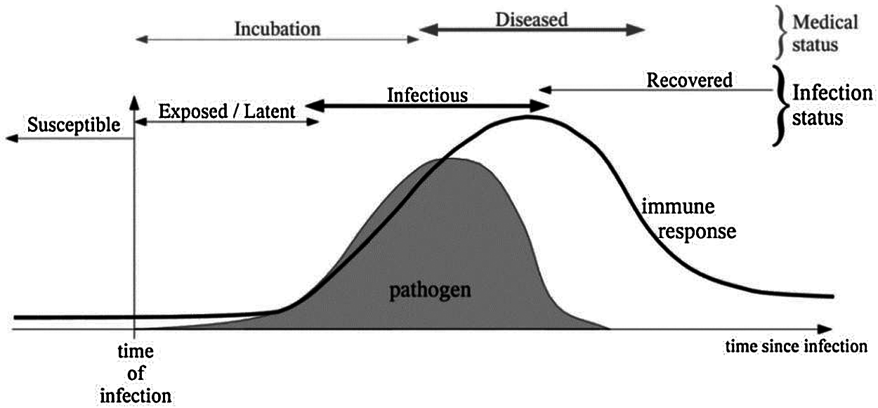
Figure 1: Pathogen infection time-line

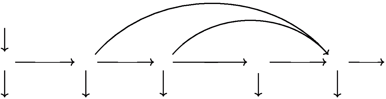
Figure 2: Schematic diagram for COVID19-SEIQRS model

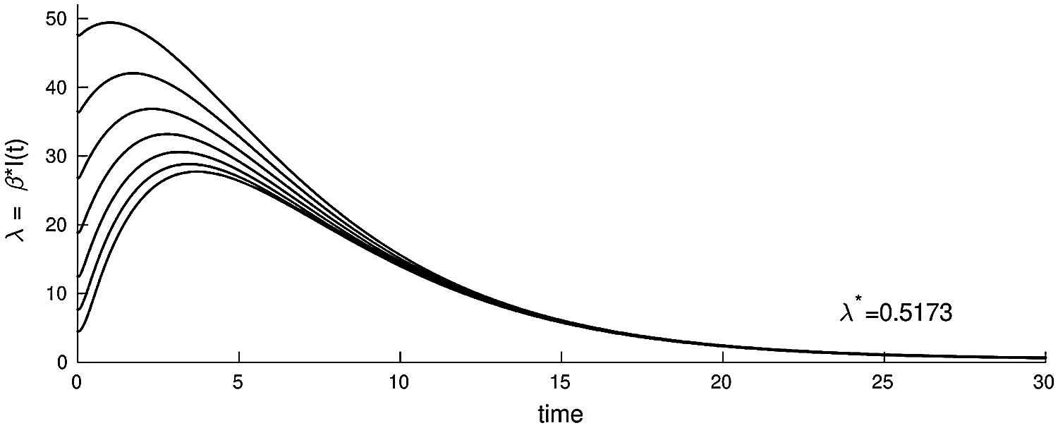
Figure 3: The plot of the infected nodes in model (3.1), λ = βI(t), as a function of time with parameters (b, β, γ, ξ, ε, μ, δ, θ, ζ, d) = (0.003, 0.32, 0.10, 0.13, 0.31, 0.001, 0.0013, 0.002, 0.0015, 0.0001)

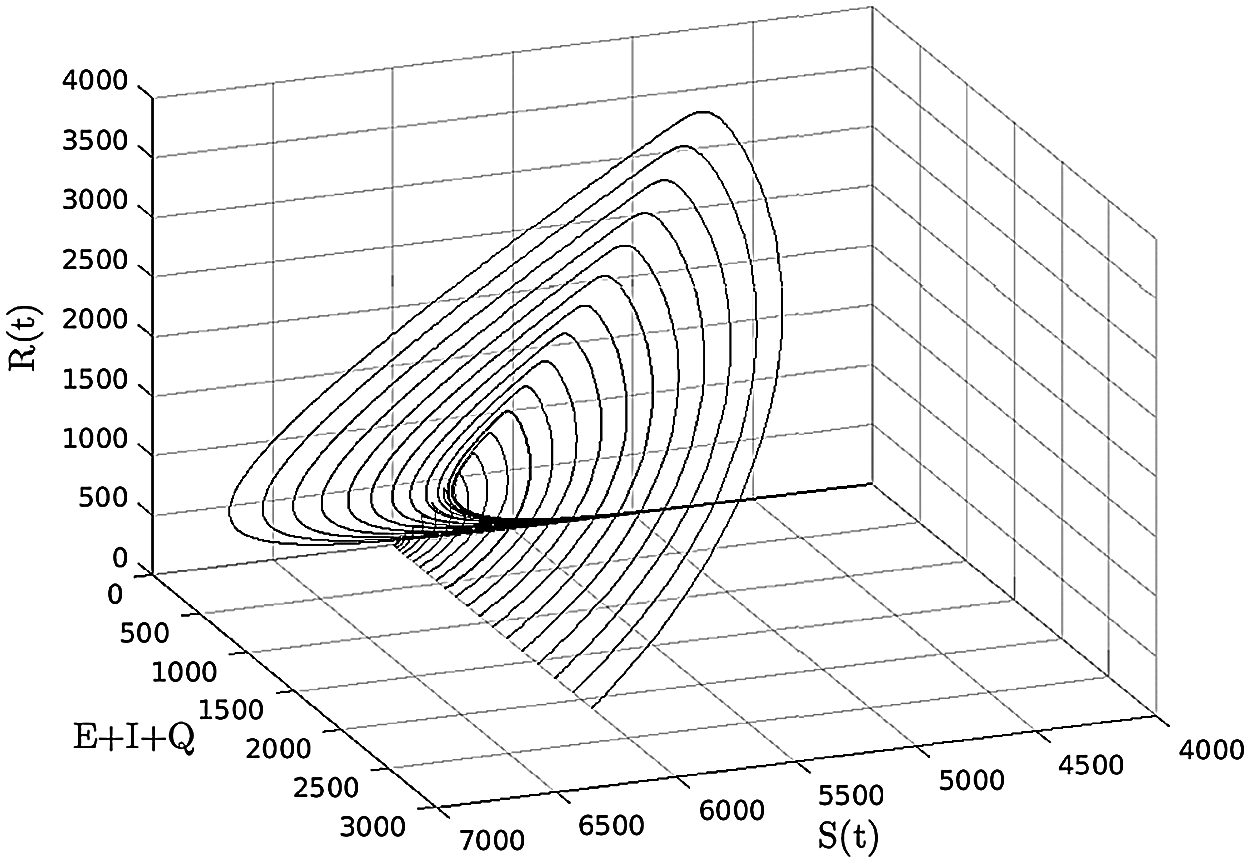
Figure 4: (S, E + I + Q, R) −space, (b, β, γ, ξ, ε, μ, δ, θ, ζ, d) = (0.003, 0.32, 0, 0.13, 0.31, 0.001, 0.0013, 0.002, 0.0015, 0.0001)

In [16] the authors introduced a SEIR model for the analysis of the COVID-19 outbreak in Wuhan, China. This model uses public data obtained from the National Health Commission of China in the period 20 Jan.–09 Feb. 2020. This model estimated key parameters of the epidemic and predicted infection spread as well as possible ending time in five different geographical areas. Optimistic estimation predicted that the epidemic ends within two weeks in Beijing and Shanghai, with strong anti-epidemic measures meaning a middle of March estimate for the rest of China. According to data up to 15th Feb. 2020, Wuhan was expected to remain infected until the beginning of April 2020. Reference [17] proposed a modified Susceptible-Infected-Recovered (SIR) model for the analysis of the transmission dynamics of infectious pathogens with susceptibility effect taken into account. They also presented Non Standard Finite Difference (NSFD) Scheme: A time-delay SIR model based on unconditionally convergent numerical model. The authors showed that NSFD must exhibit identical behavior found in the continuous model from the perspective of essential parameters including positivity, stability, dynamical consistency as well as solution boundedness for all delay factors and time intervals. The two models above are distinct due to the latency (Exposed) class located in the SEIR model, which tends to delay the peak of the outbreak; both models consist of a set of nonlinear differential equations solved using numerical iterative techniques [18]. Much of the work we analyzed as a background for the proposed work in this article seems to suffer from inherent discrepancies in their prediction power; this comes as a consequence of mixing confirmed cases (Quarantine class) with anonymous cases (Infectious class) which are directly transmitted to the Recovered class.

The mathematical modeling and simulation proposed in this article highlights the significance of this Quarantine class. Another important distinction of the proposed model is the supposition that if the entire population is inherently susceptible and converting into the Recovered category it is still no guarantee of immunity. The basis on which a Quarantine class was added is imputed to the nature of the data and this class's importance in elucidating the actual precautions being taken in Jordan; adding the Quarantine category is rather common when modeling infectious disease as in [18,19]. Although there is no direct relation in the equations between the Quarantine class and the Infectious class, nonetheless the effect of adding this class is most apparent on the speed of the outbreak spread along with 129 contacts within the population which, in turn, impacts the transmission rate of the disease.

The proposed, SEIQRS model encompasses several other parameters including the incubation period which is reflected in the constant rates of the model such as the immunity rate of the disease. Constant rates have a strong impact on the credibility of the model in terms of outbreak value and time, all constant rates have been chosen to best emulate the actual conditions in Jordan; it is common that several constant rate values fit the model felicitously however give inconsistent predictions. Optimization of the constant rate values is applied using mathematical algorithms that ensure convergence of the global minimal at effective speed. This simulator will predict the trends of the rates of Susceptible (S), Latent (E), Infectious (I), Quarantined (Q) and Recovered (R) groups. Overtime prevailing the peak value of the infectious population, the number of days for the peak of the infectious population and the number of days where the entire susceptible class population shifts into the recovered class simultaneously (this value highlights the mortality rate). In the proposed model, immunity is not conferred; the derivation and structure of the proposed model are described in the next section. In Section 3 we analyze the model, and in Section 4 we introduce numerical methods and experiments conducted using this model. Finally, in Section 5 we conclude the proposed work.

2  Proposed Model Derivation

The main parameters of the proposed model represent Susceptible (S), Latent (E), Infectious (I), Quarantined (Q) and Recovered (R) class of cases. Numerical methods are applied in order to solve the resulting set of ordinary differential equations (ODEs). The dynamic behavior is as follows: Susceptible nodes first go through a latent period (and are said to become exposed). Next, Infected persons may be asymptomatic and recover without being noticed; this is represented by moving from class I to class R. The remainder of the infected persons who show symptoms will go to Quarantine class. Since the acquired immunity is not permanent, the recovered persons may still return to the susceptible class.

Model Parameters Description: The total population size N(t) = S(t) + E(t)+ I(t)+ Q(t)+ R(t) may depend on the time variable. Here S(t), E(t), I(t), Q(t), R(t) denote the cardinality of S, E, I, Q, R compartments at time t, respectively. The per capita contact rate β, is the average number of effective contacts with other nodes per time unit. The number of new infections is denoted by βSI. b is the recruitment rate of susceptible nodes to the population. d is the per capita natural mortality rate, γ is the rate for nodes leaving the exposed compartment E for infective compartment I, δ is the rate of leaving the infective compartment I for quarantine compartment. μ is the disease related death rate in the infected compartments εI and θQ are the rates at which nodes recover temporarily after recovered (negative test result) and return to recovered class R from compartments I and Q respectively, ζ is the loss of immunity rate. In this SEIQRS model, the flow is from the S class to the E class, E class to the I class, and then directly to the R class or to the Q class and then to the R class and as the recovery is not permanent in the world, it again returns back to the S class. Fig. 2 shows the schematic diagram of the SEIQRS model.

3  Mathematical Model Derivation and Analysis

A population of nodes of size N(t) is partitioned sub-classes: Susceptible, Exposed (Infected but not yet Infectious), Infectious, Quarantined, and Recovered, with sizes denoted by S(t), E(t), I(t), Q(t), R(t) respectively. The SEIQRS model is:

dSdt=b−βSI+ζR−dS,dEdt=βSI−(γ+ξ)E−dE,dIdt=γE−(ϵ+δ)I−(μ+d)I,dQdt=δI−θQ−(μ+d)Q,dRdt=ϵI+θQ+ξE−ζR−dR, (3.1)

on the closed, positive invariant set D={x=(S,E,I,Q,R)∈R5:xi≥0,S+E+I+Q+R≤bd}

3.1 Model Analysis

Theorem 3.1: The closed set D={x=(S,E,I,Q,R)∈R5:xi≥0,S+E+I+Q+R≤bd} is positive invariant.

proof:

Let N = S + E + I + Q + R then dNdt=dSdt+dEdt+dIdt+dQdt+dRdt .

Using the main model (3.1) to get dNdt=b−dS−dE−dI−dQ−dR−μQ−μI=b−dN−μ(Q+I) ⇒ dNdt≤b−dN

hence, a standard theorem [20], can be used to prove that

N(t)≤N(0)exp (−dt)+bd(1−exp (−dt)) , in particular if N(0)≤bd , then N(t)≤bd as required this shows that D is positively invariant and that the dynamics of the basic model (3.1) are well-posed epidemiologically and mathematically.

Reproduction number and equilibrium points: The proposed SEIQRS is virus-free at P0=(bd,0,0,0,0) . Following the work in [21,22], the linear stability of P0 can be established using the next generation operator method on system (3.1). The matrices, F (for the new infection terms) and V (of the transition terms) are as follows:

It follows then that the basic reproduction number, denoted by R0, is given by

where ρ(FV−1) is the spectral radius of FV−1.

3.2 Stability of Equilibrium Points

Suppose b = (μ + d)[I + Q] + dN which means there is changing in population size (i.e., N(t) = N is constant). Therefore, S(t) + E(t) + I(t) + Q(t) + R(t) = N then Q = N − S − E − I − R so the system (3.1) can be reduced to:

dSdt=b−βSI+ζR−dS=0,dEdt=βSI−(γ+ξ+d)E=0,dIdt=γE−(ϵ+δ+μ+d)I=0,dRdt=ϵI+θ(N−S−E−I−R)+ξE−ζR−dR=0, (3.2)

Theorem 3.2: When R0 ≤ 1, the unique virus-free equilibrium P0 is locally asymptotically stable in the model (3.1).

The Jacobian matrix at free equilibrium is

J(P0)=(−d0−bβdζ0−(γ+ξ+d)bβd00γ−(d+μ+δ+ε)0−θξ−θε−θ−d−θ−ζ) (3.3)

without loss of generality, we suppose b = d, the corresponding eigenvalues of (3.3), are

where ϕ = γ + ξ + d and ψ = d + μ + δ + ε.

Clearly λ1,  λ2,  λ3 < 0 (negative), also λ4 < 0 when R0 ≤ 1, we have

Bγ<ϕψ (3.4)

therefore,

According to the stability theory in [23] we know that the sufficient conditions are all eigenvalues for the model (3.1) to be locally asymptotically stable.

Theorem 3.3: The disease-free equilibrium, P0=(bd,0,0,0,0) , of the model (3.1), is globally asymptotically stable if R0 < 1, and is unstable if R0 > 1.

Proof: Consider a Lyapunov function L = γE + (d + ξ + γ) I If R ≤ 1, then L′ = I[bγβ + (d + ξ + γ)(d + δ + ε + μ)] ≤ 0 and L′ = 0 if and only if I = 0.

Because R0 ≤ 1, it can be shows that dLdt≤0,∀E,I∈D.

Also, dLdt=0 . if and only if E = 0 and = 0, meaning the singleton P0=(bd,0,0,0,0) .

Moreover, L → ∞ as E → ∞ or I → ∞, it follows from Lasalle Invariance principle P0 is globally asymptotically stable.

The second equilibrium point of the steady state of system (3.1) is computed when R0 > 1, as shown in Fig. 3 (epidemic solution).

Hence, the unique epidemic equilibrium P∗=(S∗,E∗,I∗,Q∗,R∗)∈D exists,

with S∗=bdR0 , E∗=βS∗I∗γ+ξ+d , I∗=γE∗ϵ+δ+μ+d , Q∗=δI∗θ+μ+d R∗=ϵI∗+θQ∗+ξE∗ζ+d

and N∗=S∗+E∗+I∗+Q∗+R∗ , (S, E + I + Q, R)–space described in Fig. 4.

4  Numerical Methods and Experiment Discussion

In this section we applied the analysis using Matlab [24] to validate the mathematical model. This experiment represents data from Jordan [25], the total number of confirmed cases in the periods (16-Mar-2020, to 1-May-2020), (16-Aug-2020 to 14-Sept-2020) and (16-Sept-2020, to 1-Nov-2020) are shown in Figs. 5–7 respectively. (Continuous curve is for predicted cases and dotted curve is for actual ones.)

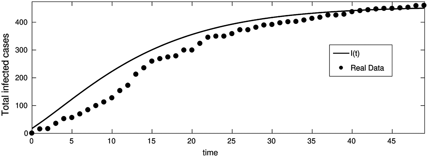
Figure 5: Total infected cases in Jordan from 16-Mar-2020 to 1-May-2020 (First wave of COVID-19 hits Jordan)

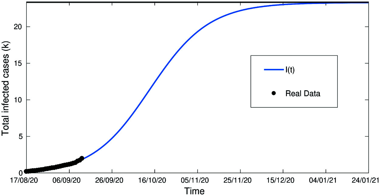
Figure 6: Total infected cases in Jordan from 16-Aug to 14-Sept (Second wave of COVID-19 hits Jordan)

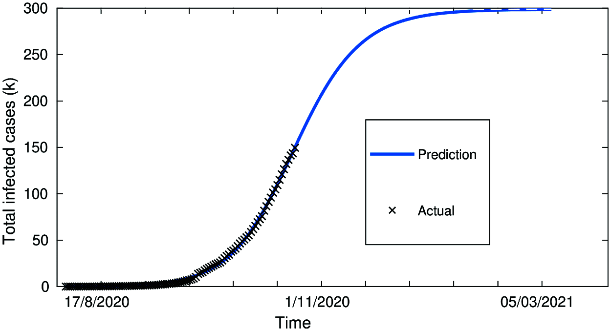
Figure 7: Total infected cases in Jordan from 16-Sept to 1-Nov (Second wave of COVID-19 hits Jordan)

From Figs. 5–7 we have covered a sufficiently long timespan including two infection waves/peaks in Jordan; It can also be seen that the accuracy of the model in terms of actual vs. predicted cases is quite close. Fig. 5 shows two data curves comparing real cases against predicted ones for the 1st wave in Jordan period 16-Mar-2020 to 1-May-2020 and clearly demonstrates the prediction model's accuracy especially towards the end of the period.

Fig. 6 which represents the period of the 2nd wave in Jordan between 14-AUG-2020 and 14-Sept-2020 has a very high accuracy.

Fig. 7 covering the extension of the 2nd wave in Jordan from 16-Sept-2020 to 1st-Nov-2020 with close to 100% fit/accuracy in predicted cases. Fig. 8, below, shows the evolution of confirmed cases with a control strategy, compared to the infected cases without any control strategy (3.1). This demonstrates the notable effect of the control strategy to decrease the number of infected nodes, and the zero-case day will come fast (decrease the quarantined period).

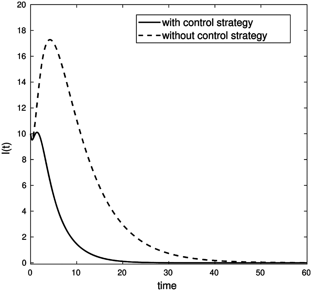
Figure 8: Comparison of infected nodes I(t) with and without a control strategy

Fig. 9, below, shows that the optimal control value ξ(t) increment in the early stages and eventually tend to be fixed. Thus demonstrating that expanding a control strategy such as vaccination, social distancing and quarantine measures need to be carried out.

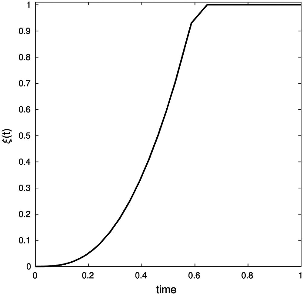
Figure 9: Optimal control ξ(t) values for certain control strategy (b, β, γ, ε, μ, δ, θ, ζ, d) = (0.001, 0.13, 0.01251, 0.1, 0.0021, 0.121, 0.032, 0.123, 0.134) with conditions (S0, E0, I0, Q0, R0) = (900, 5, 10, 0, 0) and λ1(1) = λ2(1) = λ3(1) = λ4(1) = λ5(1) = 0 on time interval [0, 450]

Fig. 10 shows that when (a trade-off factor) ϕ increases, the vaccine investment costs function Ccost(I) increases accordingly. Thus, one can conclude that there is a direct proportional correlation between ϕ and Ccost(I).

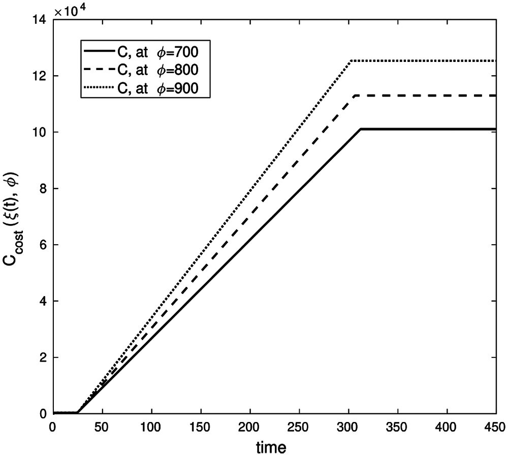
Figure 10: Cost investment function, with parameters values (b, β, γ, ε, μ, δ, θ, ζ, d) =  (0.003, 0.32, 0.1, 0.13, 0.31, 0.001, 0.0013, 0.002, 0.0001) with conditions (S0, E0, I0, Q0, R0) = (900, 5, 10, 0, 0) and λ1(450) = λ2(450) = λ3(450) = λ4(450) = λ5(450) = 0 on time interval [0, 450]

Fig. 11 describes the economic loss caused by the infected cases for different values of Φ (the average loss caused by a single infected case per day).

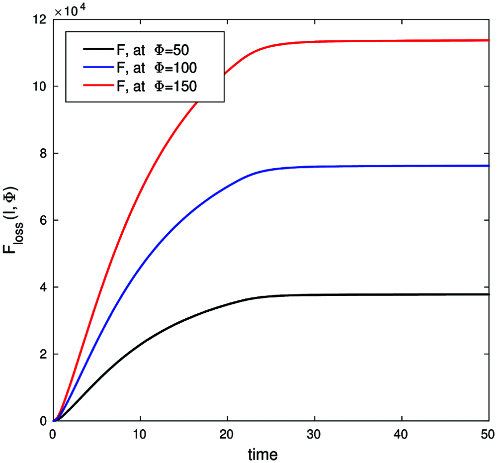
Figure 11: Economic loss function, with parameters values (b, β, γ, ε, μ, δ, θ, ζ, d) = (0.003, 0.32, 0.1, 0.13, 0.31, 0.001, 0.0013, 0.002, 0.0001) with conditions (S0, E0, I0, Q0, R0) = (900, 5, 10, 0, 0) and λ1(50) = λ2(50) = λ3(50) = λ4(50) = λ5(50) = 0 on time interval [0, 50]

Figs. 10 and 11 support the argument that the lack of a control strategy will introduce adverse economic effects due to the increase in infected cases exponentially over time with insufficient time for economic recovery.

5  Conclusions

In this article, we proposed the SEIQRS model to describe the dynamic behavior of COVID-19 infection rates in humans. The model analysis was described and the local and global stability of this model has been proven. Despite the simplicity of the model, it considers the most likely scenarios for the spread of COVID-19. The model is broad in its scope and caters for several parameters including varying timespans and infection waves; it represents a powerful instrument that can provide strategic support for decision makers in healthcare and related areas of policy and administration.

Funding Statement: The authors received no specific funding for this study.

Conflicts of Interest: The authors declare that they have no conflicts of interest to report regarding the present study.

This work is licensed under a Creative Commons Attribution 4.0 International License, which permits unrestricted use, distribution, and reproduction in any medium, provided the original work is properly cited.